Using lagged covariances in data assimilation

Abstract

This paper describes a novel method to incorporate significantly time-lagged data into a sequential variational data assimilation framework. The proposed method can assimilate data that appear many assimilation window lengths in the future, providing a mechanism to gradually dynamically adjust the model towards those data. The method avoids the need for an adjoint model, significantly reducing computational requirements compared to standard four-dimensional variational assimilation. Simulation studies are used to test the assimilation methodology in a variety of situations. The use of lagged covariances is shown to provide robust improvements to the assimilation quality, particularly if data at multiple lags are used to influence the cost function in each window. The methodology developed can be used to improve contemporary global reanalyses by incorporating time-lagged observations that may otherwise not be exploited to their full potential.

Keywords:

• long-window data assimilation
• lagged covariances
• reanalysis

1. Introduction

The process of data assimilation has been used to produce many atmospheric and oceanic reanalyses. A variety of data assimilation techniques are employed operationally, such as variational minimisation (Talagrand and Courtier, 1987), ensemble-based methods (Evensen and van Leeuwen, 2000; Bishop et al., 2001) and hybrid approaches (Fairbairn et al., 2014; Goodliff et al., 2015). A feature common to many of these methods is the partitioning of the observational data into a sequence of assimilation time windows. The estimated state trajectory, known as the analysis (), is then produced by running the assimilation procedure sequentially through the windows. The analysis in a particular window is determined by optimally combining the observations within that window and the initial guess, or background (), coming from the analysis in the previous window.

In operational global reanalyses of oceanic and atmospheric data, the length of the assimilation window typically ranges from 6 h (for atmospheric reanalyses) to 10 days (for ocean reanalyses). In general, a longer window enables more observations to be consistently analysed together, which reduces initialisation shocks and requires fewer computationally expensive assimilation steps. On the other hand, the chaotic nature of the ocean and atmosphere means the determination of an accurate solution with long time windows is more challenging. For example, in four-dimensional variational assimilation (4DVar) the tangent linear model must be computed at each time step through the window when performing the minimisation, and a long window may mean that the linearised background state does not remain valid.

Various methods have been developed to allow longer windows to be used, such as quasi-static variational assimilation (Pires et al., 1996; Swanson et al., 1998). Overlapping time windows (Sugiura et al., 2008; Köhl, 2015) can also help to overcome the tendency of the sequential procedure to lead to discontinuities between each long window. The Kalman smoother (Ménard and Daley, 1996) runs both forward and backward in time through each window and permits longer windows to be used. The Kalman smoother is equivalent to weak constraint 4DVar, which allows for model error (Fisher et al., 2005).

The use of long-window 4DVar in high-resolution atmospheric and oceanic reanalyses is extremely expensive. The aim of this paper is instead to adapt a conventional sequential short window assimilation approach by introducing additional ‘outside-window’ data, for use in particular situations where the time-lagged covariance relationships to the outside-window data are fairly robust and state-independent. In particular, we aim to use current data to influence model fields at a much earlier time in order to achieve a smoother state which is more consistent with observations.

Ultimately the methods developed here are targeted at reanalysis applications for which short-window assimilation techniques are already in operational use and the incorporation of information from observations on time scales that significantly exceed the length of the assimilation window would be beneficial.

The paper is organised as follows. Section 2 contains a description of the methodology and Section 3 presents simulation studies. Conclusions are given in Section 4.

2. Methodology

This section describes the procedure by which lagged data can be introduced into an assimilation framework. The standard method of variational assimilation is introduced in Section 2.1. The development of lagged covariance relationships and the use of these relationships to assimilate outside-window data is described in Section 2.2. Finally, the form of the observation error covariance matrix used in the lagged data assimilation is described in Section 2.3.

2.1. Standard variational assimilation

Incremental variational assimilation proceeds by determining the increments () that must be added to the background in order to minimise the cost function(1)

where the two terms on the right-hand side are the background and observation cost functions, respectively. In the formulation considered here the increments are determined at time , the start of the window. In 4DVar the two cost function terms take the form (2) (3)

where is the background error covariance matrix and are vectors of ‘within-window’ observations with error covariance matrices located at times ; there are K such observation times. The non-linear forward model operator transforms a state from time to , and is the observation operator that transforms the model state into observation space at . The matrices and are the tangent linear versions of these operators. The background at is denoted .

Throughout the assimilation window the model is linearised around the trajectory of the background state. The innovation vector is the offset between the observations and the background at . The formulation presented above is ‘strong constraint’ 4DVar for which there is no model error term.

The adjoint of is required to minimise the 4DVar cost function. The 3DVar approximation assumes that each observation is valid at the same time, usually the centre of the window, thus dispensing with altogether. The 3DVar-FGAT (First Guess at Appropriate Time) version only assumes that the innovations are valid at the same time, thus replacing the linearised adjoint with in Equation 3(3) . The 3DVar-FGAT method is commonly used in several operational assimilation centres, especially for ocean data assimilation (Balmaseda et al., 2013; Waters et al., 2015; Jackson et al., 2016).

Once the increments have been determined, the analysis is produced by adding the increments to the background state. Incremental analysis update (Bloom et al., 1996) (IAU) is commonly used to spread the influence of the increments through the window in order to produce a smoother analysis trajectory. The value of the analysis at the end of the current window is used to initialise the background state at the start of the next window.

2.2. Two-stage assimilation using lagged covariances

When considering outside-window data we introduce the additional innovation vector , defined in relation to an initial predetermined trajectory . The notation distinguishes the outside-window innovations from their within-window equivalents . The determination of , which must span the entire timescale across which the lagged covariances are to be used, is the first of two stages in the proposed methodology. Here, we will define to be the initial analysis trajectory produced by a 3DVar-FGAT reanalysis, obtained without incorporating the outside-window data.

We wish to determine the final analysis state by adding an increment vector to the trajectory . To do this requires the outside-window innovations(4)

to be calculated, where is the outside-window data and is the relevant observation operator. The innovations are calculated at all times at which outside-window data occur.

The standard linear regression relationship (e.g. McCullagh1989McCullagh and Nelder (1989)) between the increments and the innovations at a given time lag gives the expected value(5)

where is the lagged covariance matrix between and , and is the autocovariance of the increment vector. The matrix is assumed to be state-independent and may, for example, be determined using a long model run or an ensemble of short model runs. Here we consider the case of a long model run. This run is used to produce sample matrices, denoted and , which cover the spatial domains corresponding to and , respectively, and are sampled at many time points. Ordinary least squares can be used to estimate by minimising the squared norm of the residuals(6)

The minimisation can be performed using methods such as singular value decomposition (SVD), which is numerically more stable than calculating , particularly if the system has a large number of spatial points.

Given and the measured values of it is then possible to calculate the most desirable value of by introducing the new cost function term:(7)

where is the error covariance matrix of the outside-window data, discussed further in Section 2.3.

In the second stage of the assimilation the total cost function is modified to include the lagged covariance term, which for consistency must be expressed as a function of :(8)

where is the increment required relative to the background state in the second run, . In general can be sampled from the background trajectory at any time in the assimilation window as long as the lag relative to the outside-window data is valid and is sampled at the same temporal point within the window. The value of is in general different to because follows a different trajectory to . This discrepancy can be accounted for by centring around :(9)

where the background offset and modified innovations are, respectively,(10) (11)

In this form the term can be easily included in preexisting operational data assimilation algorithms. In the context of this paper the and terms in Equation 8(8) take the same form as in the first assimilation stage. The total cost function is solved using the 3DVar-FGAT assumptions and IAU is then used to produce .

The background offset will vary through time during the assimilation run. In the limit in which has no effect, will be zero at all times. If becomes zero during the second assimilation stage then the first and second assimilation trajectories are offset such that does not influence the second trajectory further.

The modified innovations (Equation 11(11) ) will influence the increments in all assimilation windows which appear at appropriate lags relative to the outside-window data. The most general form of the lagged covariance term is thus(12)

where the sum runs over the L sets of observations, each of which appears at its appropriate lag. The quantity is the error covariance matrix of the set of observations at lag l. The term is very similar to the term except the product is replaced by . The matrix can therefore be thought of as a linearised observation operator which relates the current model state to significantly time-lagged data. The adjoint of the tangent linear model is not required in , which significantly reduces the computing requirements. Furthermore the matrices can be precomputed prior to performing the assimilation. The summation in Equation 12(12) assumes that the error covariances between observations at different lags are exactly zero, but this could be extended to account for cross-lag correlations.

Figure 1. The proposed method to incorporate lagged covariances for the case in which future data influence the current assimilation trajectory. The thin burgundy line indicates the analysis produced in the first assimilation run (), the dashed blue line indicates the background in the second assimilation run () and the thick orange line indicates the analysis in the second assimilation run (). The innovations between the future data and (the model state transformed into observation space) are denoted and are separated from the start of the current assimilation window by lags . The innovations, together with the matrices , are used to influence the increments () at the start of the current window. The difference between the first and second assimilation runs at this point () must be considered when determining . The dashed extensions to indicate the lags that were used for the assimilation in the previous window, for which the corresponding may be different.

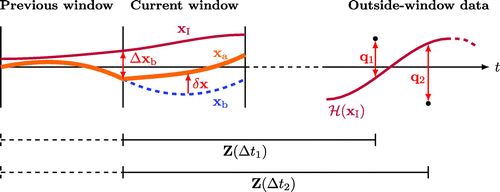
A schematic of the assimilation method is shown in Fig. 1. The situation for which the outside-window data influence the increments in two successive assimilation windows is shown.

2.3. Observation error covariance matrix

The error covariance matrix of the outside-window observations at lag l, , has two contributions. The first is from , the error covariance of the observations themselves; this independent of the particular lag chosen. The second contribution is due to the error inherent in the model used to determine the matrix ; if this error is large, the value of in the term will be inaccurate. The error is potentially lag-dependent and can be estimated using a second long model run which is assumed to represent the truth. This run is sampled many times producing the vectors and , which are analogous to and sampled from the first run. The matrix of offsets between the true values of and those predicted from at lag l is(13)

The resultant error covariance matrix is(14)

where is the total number of points sampled. The total error covariance matrix used in the term at lag l is therefore(15)

The term accounts for the accuracy of the matrix in relating the current model state to significantly time-lagged data. If the assumption of state independent covariances is violated (due to e.g. non-stationarity) the term will be large, ensuring the term is downweighted and does not bias the overall minimisation.

3. Simulation study

A simulation study is performed to test the lagged covariance assimilation methodology. The simulation models are described in Section 3.1 and results are given in Section 3.2.

3.1. Simulation models

Two models are used to test the lagged assimilation methodology. The first describes linear advection on a periodic domain, with governing equation(16)

where C is the dependent variable, t is time, z is the spatial coordinate and u is a constant speed.

For this model the two-stage assimilation procedure is used to determine the best-fit increments in sequential windows. At both stages the cost function is minimised using the Newton conjugate gradient algorithm. The model domain is discretised in both space and time. Each assimilation window consists of time steps of length unit. The spatial domain is divided into equally-spaced points, with adjacent points separated by unit. The model state vector is denoted and consists of the values of C at each point on the spatial domain.

A ‘true’ model is defined and used to both generate observations and to evaluate the performance of the assimilation procedure. At the start of the assimilation, the true model is the sinusoid(17)

where the amplitude and the phase . In all subsequent time steps the system is evolved through time using the Lax–Wendroff method (LeVeque, 1992) with speed .

The second model used is the ‘Lorenz 96’ system (Lorenz1998Lorenz and Emanuel, 1998). This system occurs on a periodic domain and has governing equation(18)

where C is the dependent variable, is the spatial coordinate with index and F is a forcing parameter which governs the extent to which chaos plays a role in the evolution of the system.

The two assimilation stages for the linear advective system are described in Sections 3.1.1 and 3.1.2. The two-stage assimilation of the Lorenz 96 system is set up in a similar way to that for the linear advective system, substituting the model parameters where appropriate. An ensemble of 100 assimilation runs is generated, using different data in each case. This enables the magnitude of any improvement to be determined more robustly than just using one realisation of the simulation.

3.1.1. First assimilation stage

The within-window observations are generated at one spatial point () and every 100 model time steps, such that there are 10 observations per window. The observations are perturbed by adding noise drawn from a Gaussian distribution of mean 0 and variance 0.05. These within-window observations are assimilated using the 3DVar-FGAT method in order to produce the trajectory .

The forward model used in the assimilation is chosen to be slightly different from the true model, in order to emulate the imperfect knowledge inherent in an operational assimilation; the forward model has amplitude , phase , and speed . The incorrect amplitude and phase produce a non-zero error in the initial state, whereas the incorrect speed governs the evolution of the system through the entire assimilation period. The forward model is used in three contexts: the first is in the variational assimilation itself, the second is to estimate the background error covariance matrix , and the third is to determine the matrices as described in Section 2.2.

Once the increments have been determined, the IAU procedure is used to smooth the analysis as follows. The analysis at the first time step, , is equal to , where is a weight whose form is described below. The analysis at subsequent time steps is(19)

where is the operator that translates a model state from one time step to the next. The weights are equal to at all time steps, which applies the increments evenly throughout the assimilation window.

3.1.2. Second assimilation stage

The outside-window observations are located at and influence increments located at a different region of the spatial domain (). The time series of outside-window data is generated by adding noise drawn from a Gaussian distribution with mean 0 and variance 0.001 to the true model. The variance used is smaller than for the within-window observations in order to clearly demonstrate the benefit of the lagged methodology. In Section 3.2.3 it is shown that a larger variance does not affect the conclusions. The observation operator is trivial because the observation locations coincide with the model grid; the outside-window innovations are therefore equal to the difference between the observations and model at the relevant spatial and temporal locations. Each outside-window observation influences the entire spatial range of the increments at the appropriate lag(s).

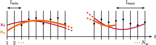
For simplicity, the outside-window data appear every 10 time units and the lags used are all integer multiples of 10 time units. The outside-window observations are therefore 10 times more temporally sparse than the within-window observations, which compensates to some extent for the lower error variance on the former. The second stage of the assimilation is only run on the first assimilation windows, where is the largest lag considered. The outside-window data which affect these windows are located at times between the minimum lag, , and inclusive. These choices, illustrated in Fig. 2, ensure that the increments in each sequential assimilation window are influenced by the same amount of data at the same set of lags.

Figure 2. The times spanned by the outside-window data and the assimilation trajectories in the simulation study. The first assimilation stage, which produces the trajectory (thin burgundy line), spans assimilation windows (indicated on the x-axis). The outside window data (black points) span times between and and are generated at the start of each window. The second assimilation stage spans times between 1 and and produces the trajectory (thick orange line). In each window the outside-window data between and in the future influence the trajectory.

The matrices are determined by running the forward model for many time steps and performing the regression in Equation 6(6) for each lag. In the simple system considered in this study, the two largest singular values of produced in the SVD procedure are found to explain essentially all of the total variance, independent of the lag. The spatial patterns associated with these values are retained and the remainder are discarded in order to reduce the influence of any residual noise.

3.2. Results

In this section, various simulation configurations are tested in order to verify the robustness of the method. The metric used to evaluate the success of the assimilation is the mean absolute error between the analysis and the truth () across all spatial and temporal points covered by the second stage of the assimilation:(20)

where the superscripts on and indicate the assimilation window, spatial point and time point, respectively. This metric is determined for both stages of the assimilation and the two values are consequently denoted , where the subscript indicates the relevant stage. It is particularly interesting to study the ratio between the metric obtained in the two stages:(21)

The closer is to zero the more beneficial influence has been brought by the lagged covariances. If is greater than one it indicates the use of lagged covariances has been detrimental.

Table 1. Mean and standard deviation of the assimilation metric for different scenarios. The metric and scenarios are described in the text.

Scenario
A
B
C
D
E
F
G
H
I
J

The following subsections describe the scenarios, labelled A–J, in detail. For each scenario, the mean and standard deviation of obtained in the ensemble of 100 assimilation runs are presented in Table 1. In each scenario, at least one parameter of the assimilation is varied. The results included in the table have been chosen based on a reasonable variation of the parameter(s) in question. Each subsection also contains tests of wider ranges of parameters, exploring more fully the strengths and limitations of the two-stage procedure.

3.2.1. Assimilation with single lag (A)

In the first configuration, denoted A, each outside-window observation influences just one set of increments at a single lag in one assimilation window. The lag separating the observations and increments is chosen to be eight multiples of the assimilation window length, i.e. 80 time units; the second stage of the assimilation therefore spans 920 time units. The metric is slightly lower than unity, indicating the methodology has been moderately successful. The combination of the dynamics of the forecast and the extra information from the outside-window observations has led to a more physically consistent analysis state.

3.2.2. Assimilation with multiple lags (B)

In scenario B, outside-window data at lags of 10–80 time units (in steps of 10) are used to influence the increments in each window. Each outside-window observation therefore influences the increments spanning in eight sequential windows; the increments influenced change as the procedure steps through the assimilation windows.

A large improvement in the value of is found relative to scenario A because each observation is used to influence more than one set of increments and the trajectory corresponding to the cost function term is smoothed through time.

Figure 3. Values of as a function of spatial coordinate (z) and lag (in multiples of 10 time units). Lags from 10–80 time units are considered and the z-values are restricted to the spatial domain of the increments influenced by the outside-window data. The dashed lines show the full spatial extent of the domain and the vertical line marks .

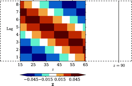
Figure 3 shows the values of at each lag, restricted to the spatial domain of the increments influenced by the outside-window data. The diagonal pattern of the largest positive covariances (the orange regions) can be explained by considering the speed of advection; shorter lags have a stronger influence closer to the innovation location ().

Figure 4. The difference between (left) the initial assimilation and the truth (right) the second assimilation and the truth for one realisation of scenario B. The spatial location of the within-window data is indicated on the left-hand plot. On the right-hand plot the locations of the outside-window innovations, and the increments that they influence, are shown.

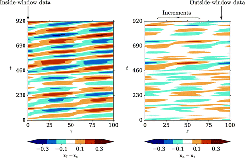
Figure 5. Time evolution of deviations between the truth and the (dashed blue line) first (thick orange line) second assimilation trajectory at for one realisation of scenario B.

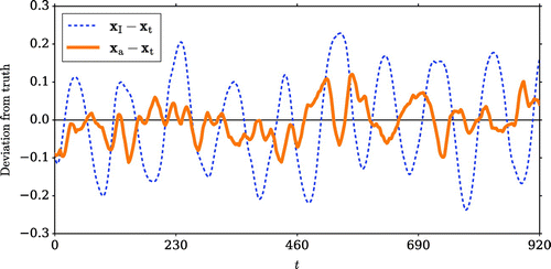
Figure 6. The dependence of the metric on the number of lags used in the assimilation.

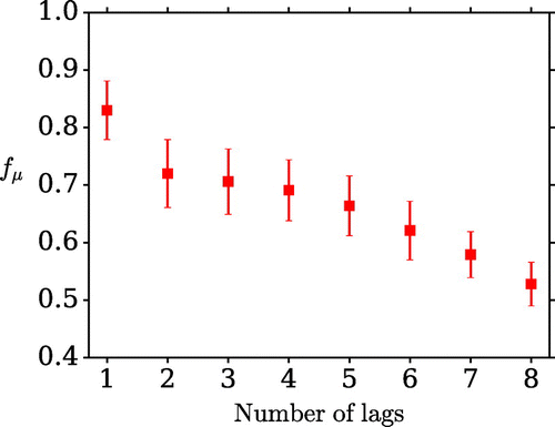
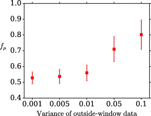
Figure 7. The dependence of the metric on the error variance of the outside-window observations.

The differences between the results of the first and second assimilation stages and the truth for one realisation of scenario B are shown in Fig. 4. Figure 5 shows the time evolution of the deviations from the truth for both assimilation stages at . A clear improvement can be seen after the second stage.

Additional results for different numbers of lags are shown in Fig. 6. When k lags are used the observations appear at [80, ..., ] time units relative to the increments that they influence. Adding more lags consistently improves the success of the method. Due to the significant benefit observed compared to just using data at one lag, all subsequent scenarios use data located at lags 10–80 in steps of 10 units.

3.2.3. Increased uncertainty on outside-window data (C)

The default error variance of the outside-window data is 0.001. In order to check whether this is making the method unrealistically effective, the variance is increased to 0.05, which is the same as the variance of the within-window data. This scenario is labelled C and, while is not as small as in scenario B, an improvement over the first assimilation stage is still observed. Figure 7 shows the results for a variety of values of the error variance on the outside-window data. As expected, the improvement over the first stage diminishes when this variance is larger.

Figure 8. The difference between (left) the initial assimilation and the truth (right) the second assimilation and the truth for one realisation of scenario D. On the right-hand plot the locations of the outside-window innovations, and the increments that they influence, are shown. The quantities on the left-hand plot extend to approximately .

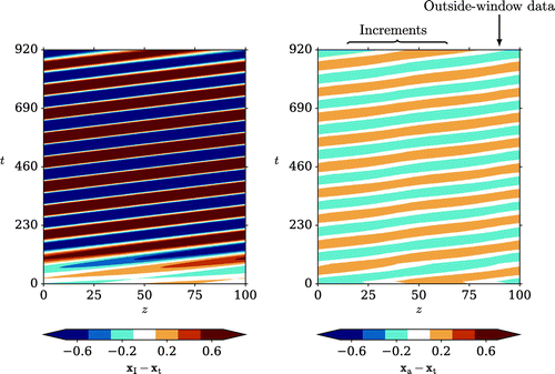
Figure 9. The dependence of the metric on the error variance of the serially correlated outside-window observations.

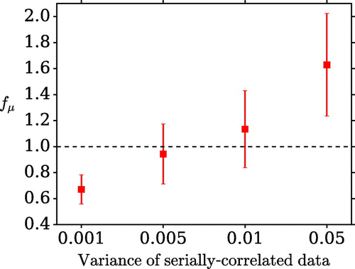
Figure 10. The dependence of the metric on the stochastic variance of the long model run used to determine the matrices.

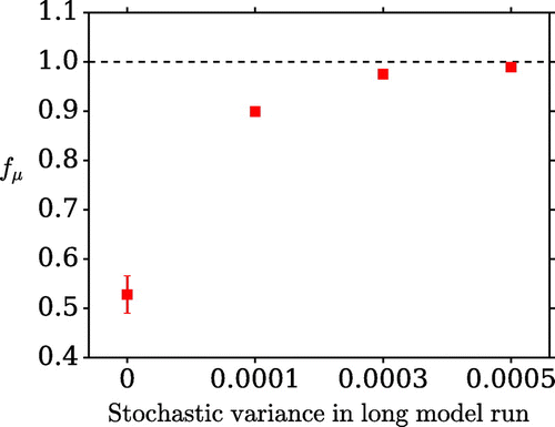
Figure 11. The dependence of the metric on the parameters of the long model run used to determine the matrices. In each case, both the amplitude and speed of the model are set to the same value.

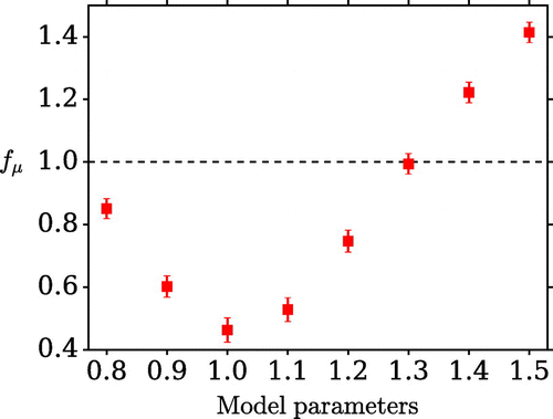
Figure 12. The dependence of the metric on the number of consecutive outside-window observations which are averaged together.

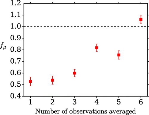
Figure 13. The dependence of the metric on the stochastic speed variance.

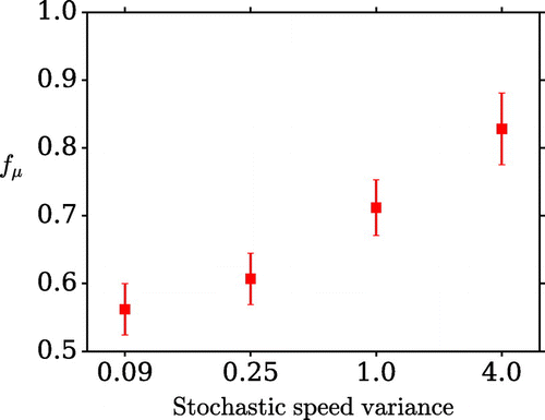
Figure 14. The dependence of the metric on the ‘Lorenz 96’ model forcing parameter.

3.2.4. No within-window observations (D)

Although the within-window observations greatly improve the accuracy of the analysis produced by the first assimilation run, it is not essential to include them in these studies. In scenario D the within-window observations are omitted entirely from the minimisation; in other words the cost function term is excluded from Eqs. 1(1) and 8(8) . The first assimilation trajectory and the truth differ by values spanning approximately , which reflects the fact that the trajectory follows exactly that of the forward model. The metric is close to zero, indicating a substantial improvement over the first stage has been achieved by including the lagged data. The differences between the results of the first and second assimilation stages and the truth for one realisation of scenario D are shown in Fig. 8.

3.2.5. Model deficiencies (E, F, G)

It is important to check to what extent the methodology is affected by deficiencies in the models used (i.e. the forward model and the model used to determine ). In the results shown above, the parameters of the forward model are already slightly different to the truth, and the method is successful. Three scenarios with further differences between these models, and between the models and the truth, are considered.

In the first scenario, E, the outside-window noise is generated as an AR(1) procedure with variance 0.001. The important feature of this scenario is that there is serial correlation present in the observations that is not present in the forward model. The results are degraded relative to scenario B but there is still an improvement moving from the first to the second assimilation, indicating the procedure is robust. Figure 9 shows results for which the same serial correlation is used but the errors are larger. As the variances increase the results degrade relatively more quickly than the equivalents in scenario C, and for larger variances the second stage has a detrimental effect. A detailed description of methods that compensate for serially correlated errors is beyond the scope of this paper, but relevant techniques can be found in e.g. Brockwell and Davis (2002).

The next two scenarios involve changes to the long model run which is used to determine . In scenario F a stochastic term is added to the long model run. A quantity drawn from a Gaussian distribution of mean 0 and variance 0.0001 is added to each spatial point before evolving the model to the next time step. The resulting matrices are therefore different to the defaults. The use of different stochastic variances is shown in Fig. 10; as this variance increases, the quality of the assimilation decreases.

In scenario G the parameters of the long model run, which by default are equal to those of the forward model, are altered; the amplitude changes from 1.1 to 1.2, and the speed from 1.1 to 1.2. These parameters are different to those used in both the truth and the forward model. In each scenario the metric indicates that there is an improvement from the first to the second stage of assimilation, but the improvement is not as large as that seen in scenario B. The results for several sets of parameters are shown in Fig. 11; in each case, both the amplitude and speed of the model are set to the same value. A larger parameter space could be explored but these numbers are reasonably illustrative.

These results, which include several values of greater than one, show the importance of using a good model to determine ; if the parameters are very different to those of the truth or the forward model, the assimilation procedure will not be reliable. Part of the reason for the degradation in this case is the fact that eight lags are used; the matrices for longer lags are determined after the model has run for longer and therefore developed larger errors. If a single lag of 10 time units is used the second stage of the assimilation still results in an improvement over the first. If the amplitude and speed of the long model run are both set to 1.0, the true value, the second assimilation stage is the most successful.

In general, if is determined with less accuracy then a degradation in the results occurs, and dynamical consistency between the forward model and the model used to determine is beneficial, even if they both differ from the true model. It is important to note that the use of data at multiple lags is usually useful in these cases; if observations at just one lag are used, the metric is potentially much worse. The modification of the model parameters in scenarios F and G is similar to the techniques known as Stochastically Perturbed Parameterisations and Stochastically Perturbed Parameterisation Tendencies (e.g. Ollinaho2016Ollinaho et al. (2016)), although those techniques are usually employed for different purposes.

3.2.6. Lower-frequency observations (H)

In scenario H every consecutive group of three outside-window innovations (spanning 30 time units) is averaged to produce one value which is then used in three sequential assimilation windows. This emulates a situation in which the outside-window observations are measured on timescales longer than the length of the assimilation window. The lags used still span 10–80 time units in steps of 10 units. The result is degraded compared to scenario B but a positive influence of the time-lagged data is still clearly seen. The results for several different averaging periods are shown in Fig. 12. The longer the averaging period, the worse the results; this is to be expected because the averaged outside-window data correspond less accurately to the truth.

3.2.7. Chaotic systems (I, J)

It is important to investigate the success of the proposed method with systems exhibiting various degrees of chaos and stochastic noise. Such effects are prominent in the ocean and atmosphere as a result of, e.g., turbulence and emulating them will provide some level of understanding of how viable the method is in operational contexts.

Two scenarios are used to test the success of the lagged assimilation method under chaotic conditions. The first scenario, labelled I, uses the linear advective system. In Scenario F a stochastic term added to the model state of this system was investigated. It is also possible to consider a stochastic speed as follows. A random speed is generated at each spatial point before evolving to the next time step. The speed is drawn from a Gaussian distribution with mean equal to the relevant value (i.e. u or ) and variance 0.09. The metric indicates an improvement from the first to the second stage. The results for several larger variances are shown in Fig. 13. As the stochastic variance increases the improvement lessens, but these results show that in principle the method is able to handle turbulent conditions.

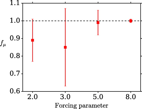
In scenario J the Lorenz 96 system is used to simulate systems with varying levels of chaos. The forcing parameter F is initially set to a low value (2) in order to limit the chaotic behaviour. In this regime, the system behaves similarly to the linear advective case and the two-stage assimilation is therefore relatively successful. The method is tested by gradually increasing F in order to produce more chaotic conditions. The results for several values of F shown in Fig. 14. As the amount of chaos increases the effectiveness of the assimilation is reduced until eventually the second assimilation stage produces no improvement over the first.

This scenario demonstrates the importance of including (Equation 14(14) ) in the matrix (Equation 15(15) ) when assimilating into systems with large amounts of turbulence. If is not included, the results of scenario J are significantly degraded when using larger values of F. For example, when the value of is when is included in but if is omitted. These results illustrate how the term accounts for the accuracy of the matrix in relating the current model state to time-lagged data.

4. Conclusions

In this paper, we have presented a method to incorporate data at significant time lags into a sequential variational data assimilation framework. The method uses state covariances determined from a model, rather than error covariances, and is performed in two stages. In the first stage a standard variational assimilation, without the lagged data, is performed. The second stage incorporates the lagged data into the first trajectory by including an additional term in the cost function.

The proposed methodology has been tested using simulation studies, considering several scenarios with a simple advective system that emulates features of contemporary large-scale operational weather and climate reanalyses. In all cases the method was shown to provide an improvement over the standard 3DVar-FGAT assimilation (except when the model used to determine the matrices is very inaccurate). The use of model dynamics to calculate the lagged covariances, and the additional information from the outside-window data, together produce a more consistent analysis state. Even if the observation term is removed (i.e. only lagged data are used, as in scenario D), the method has been shown to still be effective.

The use of multiple lags to influence each set of increments is found to be beneficial. Including multiple lags at once will provide greater dynamical consistency through time. Using each observation to influence multiple increments around the trajectory is similar in concept to the propagation of the increments throughout the assimilation window that occurs in standard variational assimilation.

Lorenc and Payne (2007) discusses the use of optimal regularisation to estimate the mean and variability of the time-evolution of a model in the context of numerical weather prediction. Parallels can be drawn between that technique and the methodology presented in this paper; Equation 18 of Lorenc and Payne (2007) is similar to our Equation 5(5) .

In scenarios E, F and G the model used to calculate is perturbed in various ways and each time the method is able to cope with the changes. Dynamical consistency between the forward model and the model used to determine is important, however; if the two models are too different, the fit result is highly degraded. The use of data at multiple lags then provides important stability if the underlying model contains errors; additionally, shorter lags enable less time for the model errors to develop and result in more accurate results. The choice of lags in an operational reanalysis should be based on both of these factors.

In scenarios I and J the methodology was tested on models with varying levels of stochastic noise and chaos in order to simulate the turbulence which occurs in real-world systems. The success of the methodology is reduced with larger levels of turbulence. The method introduced in this paper is targeted towards exploiting signals which recur robustly on long time scales, and if no such signal exists then the method will not be successful. As shown in scenario J, however, the inclusion of the term (Equation 14(14) ) in the expression of the error variance for time-lagged observations, (Equation 15(15) ), accounts for the error in the forward observation operator when a chaotic system is used for simulation.

The SVD method used to determine can be used to inform the choice of lags and the spatial extent covered. When applied to the matrix , the SVD method produces a set of spatial patterns and associated time series (Bretherton et al., 1992). Both the variance explained by the patterns and the correlation of the time series with can be used to select the lags and the spatial extent covered by . Although there is some freedom to make this selection, the term in accounts for errors in the linear forward observation operator for time-lagged observations and permits proper weights for outside-window innovations to be determined even for a suboptimal choice of lags.

The methodology described in this paper can be used in current reanalyses that use sequential variational data assimilation and for which long-window methods are computationally unfeasible. There are several processes, particularly in the ocean, that are known to involve teleconnections on multi-year time scales; as an example, the Atlantic Meridional Overturning Circulation is thought to exhibit significant time-lagged correlations with high-latitude density anomalies (Polo et al., 2014). The exploitation of such teleconnections would be desirable to improve the model state estimate. The time-lagged method described here should be effective at assimilating these data through high-latitude density increments requiring only small adjustments to the current operational 3DVar-FGAT assimilation apparatus.

Acknowledgements

We thank Nancy Nichols, Ross Bannister and Peter Jan van Leeuwen for useful discussions, and the two anonymous reviewers for their comments which greatly improved the paper.

Additional information

Funding

This work was supported by the NERC [grant number NE/M005119/1].

Notes

No potential conflict of interest was reported by the authors.

References

- Balmaseda, M. A., Mogensen, K. and Weaver, A. T. 2013. Evaluation of the ECMWF ocean reanalysis system ORAS4. Q. J. Roy. Meteor. Soc. 139(674), 1132–1161. DOI: 10.1002/qj.2063.
- Bishop, C. H., Etherton, B. J. and Majumdar, S. J. 2001. Adaptive sampling with the ensemble transform Kalman filter. Part I: theoretical aspects. Mon. Weather Rev. 129(3), 420–436. DOI: 10.1175/1520-0493(2001)129\lt0420:ASWTET\gt2.0.CO;2.
- Bloom, S. C., Takacs, L. L., da Silva, A. M. and Ledvina, D. 1996. Data assimilation using incremental analysis updates. Mon. Weather Rev. 124(6), 1256–1271. DOI: 10.1175/1520-0493(1996)124\lt1256:DAUIAU\gt2.0.CO;2.
- Bretherton, C. S., Smith, C. and Wallace, J. M. 1992. An intercomparison of methods for finding coupled patterns in climate data. J. Climate 5(6), 541–560. DOI: 10.1175/1520-0442(1992)005\lt0541:AIOMFF\gt2.0.CO;2.
- Brockwell, P. J. and Davis, R. A. 2002. Introduction to Time Series and Forecasting. Springer-Verlag, New York, pp. 137–178.
- Evensen, G. and van Leeuwen, P. J. 2000. An ensemble Kalman smoother for nonlinear dynamics. Mon. Weather Rev. 128(6), 1852–1867. DOI: 10.1175/1520-0493(2000)128\lt1852:AEKSFN\gt2.0.CO;2.
- Fairbairn, D., Pring, S. R., Lorenc, A. C. and Roulstone, I. 2014. A comparison of 4DVar with ensemble data assimilation methods. Q. J. Roy. Meteor. Soc. 140(678), 281–294. DOI: 10.1002/qj.2135.
- Fisher, M., Leutbecher, M. and Kelly, G. A. 2005. On the equivalence between Kalman smoothing and weak-constraint four-dimensional variational data assimilation. Q. J. Roy. Meteor. Soc. 131(613), 3235–3246. DOI: 10.1256/qj.04.142.
- Goodliff, M., Amezcua, J. and van Leeuwen, P. J. 2015. Comparing hybrid data assimilation methods on the Lorenz 1963 model with increasing non-linearity. Tellus A 67, 26928. DOI: 10.3402/tellusa.v67.26928.
- Jackson, L. C., Peterson, K. A., Roberts, C. D. and Wood, R. A. 2016. Recent slowing of Atlantic overturning circulation as a recovery from earlier strengthening. Nat. Geosci. 9(7), 518–522. DOI: 10.1038/ngeo2715.
- Köhl, A. 2015. Evaluation of the GECCO2 ocean synthesis: transports of volume, heat and freshwater in the Atlantic. Q. J. Roy. Meteor. Soc. 141(686), 166–181. DOI: 10.1002/qj.2347.
- LeVeque, R. J. 1992. Numerical Methods for Conservation Laws Birkhäuser, Basel, pp. 97–113.
- Lorenc, A. C. and Payne, T. 2007. 4D-Var and the butterfly effect: statistical four-dimensional data assimilation for a wide range of scales. Q. J. Roy. Meteor. Soc. 133(624), 607–614. DOI: 10.1002/qj.36.
- Lorenz, E. N. and Emanuel, K. A. 1998. Optimal sites for supplementary weather observations: simulation with a small model. J. Atmos. Sci. 55(3), 399–414. DOI: 10.1175/1520-0469(1998)055\lt0399:OSFSWO\gt2.0.CO;2.
- McCullagh, P. and Nelder, J. A. 1989. Generalized Linear Models Chapman & Hall, London, pp. 48–97.
- Ménard, R. and Daley, R. 1996. The application of Kalman smoother theory to the estimation of 4DVAR error statistics. Tellus A 48(2), 221–237. DOI: 10.1034/j.1600-0870.1996.t01-1-00003.x.
- Ollinaho, P., Lock, S.-J., Leutbecher, M., Bechtold, P., Beljaars, A. and co-authors. 2016. Towards process-level representation of model uncertainties: stochastically perturbed parametrizations in the ECMWF ensemble. Q. J. Roy. Meteor. Soc. 143(702), 408–422. DOI: 10.1002/qj.2931.
- Pires, C., Vautard, R. and Talagrand, O. 1996. On extending the limits of variational assimilation in nonlinear chaotic systems. Tellus A 48(1), 96–121. DOI: 10.3402/tellusa.v48i1.11634.
- Polo, I., Robson, J., Sutton, R. and Balmaseda, M. A. 2014. The importance of wind and buoyancy forcing for the boundary density variations and the geostrophic component of the AMOC at 26°N. J. Phys. Oceanogr. 44(9), 2387–2408. DOI: 10.1175/JPO-D-13-0264.1.
- Sugiura, N., Awaji, T., Masuda, S., Mochizuki, T., Toyoda, T., Miyama, T. and co-authors. 2008. Development of a four-dimensional variational coupled data assimilation system for enhanced analysis and prediction of seasonal to interannual climate variations. J. Geophys. Res. Oceans 113(C10), C10017. DOI: 10.1029/2008JC004741.
- Swanson, K., Vautard, R. and Pires, C. 1998. Four-dimensional variational assimilation and predictability in a quasi-geostrophic model. Tellus A 50(4), 369–390. DOI: 10.1034/j.1600-0870.1998.t01-4-00001.x.
- Talagrand, O. and Courtier, P. 1987. Variational assimilation of meteorological observations with the adjoint vorticity equation I: theory. Q. J. Roy. Meteor. Soc. 113(478), 1311–1328. DOI: 10.1002/qj.49711347812.
- Waters, J., Lea, D. J., Martin, M. J., Mirouze, I., Weaver, A. and co-authors. 2015. Implementing a variational data assimilation system in an operational 1/4 degree global ocean model. Q. J. Roy. Meteor. Soc. 141(687), 333–349. DOI: 10.1002/qj.2388.