How well can an ensemble predict the uncertainty in the location of winter storm precipitation?

Abstract

A pair of morphing-based ensemble forecast diagnostics is proposed for the verification of the location of precipitation events. The diagnostics are applied to operational global ensemble forecasts of winter storms in the United States in the winters of 2014/2015 and 2015/2016. A slowly developing systematic error is found to lead to an unrealistically fast eastward propagation of the storms in the week-two forecasts. Apart from this systematic error, the forecasts predict the uncertainty in the location of the precipitation events reliably. They, however, also grossly underestimate the uncertainty of the amount of precipitation in the short (shorter than 5 days) forecast range.

Keywords:

• ensemble verification
• precipitation
• morphing
• winter storm

1. Introduction

The predictability of a chaotic dynamical system is measured by the temporal growth of the magnitude of the errors in predictions of the system. For an Eulerian scalar state variable of a spatio-temporally chaotic system, the standard measure of the magnitude of the prediction error is the root-mean-square (rms) error, with the mean taken over the spatial domain of the system. The use of the rms error as the measure of prediction error, however, is problematic for a scalar state variable of sharp gradients, because for such a variable, the rms error indicates a rapid loss of predictability once the dominant features of the field become slightly misplaced. Intuition suggests that a proper error measure should indicate that the error is a small displacement of the dominant features. More generally, the measure should provide information about the magnitude of the displacement error, and also the errors in the amplitude and spatial structure of the dominant features.

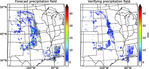
An example for a scalar field of the aforementioned type is the precipitation field associated with an extratropical or tropical cyclone, whose evolution is driven by the spatio-temporally chaotic, multi-scale dynamics of the atmosphere, which organizes it into bands with sharp boundaries and a rich and rapidly changing structure within the bands (Fig. 1). If the precipitation bands are slightly misplaced in a forecast, the rms error indicates poor forecast quality, even if the precipitation field is otherwise well predicted.

Fig. 1. An example of a slightly misplaced forecast precipitation field.

Notes: The forecast field (left) is the 24-h forecast of the 1-h accumulated precipitation starting at 0000 UTC 1 June 2005 and the verifying analysis field (right) is the 1-h accumulated Stage II precipitation analysis. In the left panel, the grey shades indicate the contours of the verifying precipitation field.

The error in the prediction of a precipitation event can be characterized, at minimum, by three error components: the errors in the location, amplitude (amount) and structure of the predicted precipitation (e.g. Wernli et al., 2008). Motivated by the work of Keil and Craig (2007, 2009) on morphing-based precipitation verification techniques and a series of papers on digital image quality measures (Wang and Bovik, 2002; Wang et al., 2004; Wang and Bovik, 2009), we have developed a technique to estimate the three error components in deterministic precipitation forecasts (Han and Szunyogh, 2016, 2017). The goal of the present study is to extend our technique for the estimation of the location error component to ensemble forecasts. In particular, we derive diagnostics for the estimation of the systematic location error and the verification of the “spread-skill relationship” (e.g. Buizza, 1997) for the location. We apply the two diagnostics to operational global ensemble forecasts of the 32 United States winter storms that were named by The Weather Channel in the winters of 2014/2015 and 2015/2016.¹ We note that a recent study (Greybush et al., 2017) based on the examination of forecasts of two of the storms from the same winters showed the importance of using the ensemble approach for the prediction of winter storms.

2. Methodology

We assume that the location of a precipitation event can be described by a two-dimensional vector of location $\mathit{r}$. While the verification technique we propose does not require the knowledge or estimation of $\mathit{r}$, the assumption that the position of the event can be described by a single location $\mathit{r}$ makes its justification more transparent.² Because we consider $\mathit{r}$ a random variable, the position ${\mathit{r}}_a$ of the event in the verifying analysis is a realization of $\mathit{r}$. Likewise, the positions ${\mathit{r}}_f^{\mathit{k}}$ $(k=1,2\dots ,K)$ of the event in the K forecast ensemble members are also realizations of $\mathit{r}$.

Consider a set of verification cases, in which subsets of cases may be related to the same weather event at different verification times. Let M be the total number of verification cases. For each verification case m(m = 1, 2, …, M), we consider all ensemble forecasts from an archived data-set that are valid at the (verification) time of the case. While there are different lead time forecasts for each case, not all ensemble members predict a storm at each lead time. We therefore introduce the notation $K^{\prime }\left(m,t_f\right)$, $K^{\prime }\left(m,t_f\right)\le K$, for the number of ensemble members that at lead time t_f include a precipitation event that may be related to winter storm $m\left(m=1,2,\dots ,M\right)$. (We will give a formal definition of “may be related” shortly.) Our goal is to verify the ensemble-based prediction of the mean and standard deviation of the conditional probability distribution of $\mathit{r}$ subject to the condition that the forecast verification feature may be related to an observed winter storm.

Our task has two parts. First, we have to identify the ensemble members that include a precipitation event that may be related to a verifying event. Second, we have to verify the ensemble-based estimates of the statistical parameters of the conditional probability distribution of $\mathit{r}$ for the collection of cases that we identify. The only information available to us at the beginning of the process is the knowledge of the fields of verifying precipitation data $P^a\left(m\right)\left(m=1,2,\dots ,M\right)$ in a search region, which is selected such that the verifying event is at about its centre, and the related K-member ensembles of forecast precipitation fields $P^k\left(m,t_f\right)\left(k=1,2,\dots ,K\right)$.

We use the technique of Han and Szunyogh (2017) to first find a shift vector $d{\mathit{X}}^k(m,t_f)=\left(d{U}^k(m,t_f),d{V}^k(m,t_f)\right)$ for each ensemble member k, forecast case m and lead time t_f that corrects the location error. (dU^k(m, t_f) and dV^k(m, t_f) are the zonal and meridional component of $d{\mathit{X}}^k(m,t_f)$, respectively.) Formally, the shift vector that “corrects the location error” is the vector that shifts P^k(m, t_f) such that it maximizes the similarity between P^a(m) and the shifted P^k(m, t_f) field, $P_{\mathit{shift}}^k(m,t_f)$. We think of $d{\mathit{X}}^k(m,t_f)$ as the difference between the location ${\mathit{r}}_a(m)$ of the verifying precipitation feature and the predicted location ${\mathit{r}}_f^k(m,t_f)$ $\left(k=1,2,\dots ,K\right)$ of the same feature in ensemble member k, that is,(1) $$d{\mathit{X}}^k\left(m,t_f\right)={\mathit{r}}_a\left(m\right)-{\mathit{r}}_f^k\left(m,t_f\right),k=1,2,\dots ,K.$$(1)

We measure the similarity between P^a(m) and $P_{\mathit{shifted}}^k(m,t_f)$ by the Amplitude and Structural Similarity Index Measure (ASSIM) (Han and Szunyogh, 2017), which is an adaptation of the Structural Similarity Index Measure (SSIM) of Wang et al. (2004) and Wang and Bovik (2009). We choose the free parameters of the measure such that it gives equal weights to the similarity of the amplitude, the similarity of the spatial variability and the point-wise correlation of the two fields. ASSIM takes a value in the closed interval [0, 1], with one indicating identical fields and a lower value indicating less similarity between the two fields. We assume that the precipitation feature of ensemble member k “may be related to” winter storm m, if ASSIM for P^a(m) and $P_{\mathit{shift}}^k(m,t_f)$ is equal to, or larger than a prescribed threshold value a. $K^{\prime }\left(m,t_f\right)$ therefore is the number of ensemble members for forecast case $m\left(m=1,2,\dots ,M\right)$ and forecast lead time t_f for which ASSIM is larger than a.

We expect $K^{\prime }\left(m,t_f\right)$ to be a monotonically decreasing function of the forecast lead time t_f and require that $K^{\prime }\left(m,t_f\right)\ge 2$ for all forecast cases used in the computation of the diagnostics at t_f. We denote the number of forecast cases that satisfy the latter condition by $M^{\prime }\left(t_f\right)$. Estimates of the statistics based on such small ensemble sizes can be included in the diagnostics, because while the sampling errors (the estimation errors due to a small ensemble) can be large for a particular case m and lead time t_f, the expected value and the standard deviation of the sampling errors are known from the theory of statistics even for such small sample sizes. In particular, if the ensemble members ${\mathit{r}}_f^k(k=1,2,\dots ,K^{\prime })$ sample the true distribution of $\mathit{r}$, the ensemble average(2) $$\overline{{\mathit{r}}_f}=\frac{1}{K^{\prime }}\sum _{k=1}^{K^{\prime }}{\mathit{r}}_f^k$$(2)

estimates the (unknown) true mean $\overline{\mathit{r}}=E\left[\mathit{r}\right]$ of the distribution with an error(3) $${\mathit{b}}_{\mathit{loc}}=\overline{\mathit{r}}-\overline{{\mathit{r}}_f},$$(3)

whose mean is(4) $$E[{\mathit{b}}_{\mathit{loc}}]=0,$$(4)

and mean-square is(5) $$E\left[{\left({\mathit{b}}_{\mathit{loc}}\right)}^2\right]=E\left[{\left({\mathit{b}}_{\mathit{loc}}-E\left[{\mathit{b}}_{\mathit{loc}}\right]\right)}^2\right]=\frac{1}{K^{\prime }}{\mathrm{\Sigma }}_{\mathit{loc}}^2.$$(5)

Here,(6) $${\mathrm{\Sigma }}_{\mathit{loc}}^2=E\left[{\left(\mathit{r}-\overline{\mathit{r}}\right)}^2\right]$$(6)

is the (unknown) true variance of $\mathit{r}$. Hereafter, $E\left[·\right]$ denotes the expected value of the random variable in the brackets. In our proposed diagnostics, this expected value is estimated by an average over the $M^{\prime }\left(t_f\right)$ verification cases.

Taking the ensemble mean of Equation (1(1) $$d{\mathit{X}}^k\left(m,t_f\right)={\mathit{r}}_a\left(m\right)-{\mathit{r}}_f^k\left(m,t_f\right),k=1,2,\dots ,K.$$(1) ) yields(7) $$\overline{d\mathit{X}}\left(m,t_f\right)={\mathit{r}}_a\left(m\right)-\overline{{\mathit{r}}_f}\left(m,t_f\right),$$(7)

where(8) $$\overline{d\mathit{X}}\left(m,t_f\right)=\frac{1}{K^{\prime }\left(m,t_f\right)}\sum _{k=1}^{K^{\prime }}d{\mathit{X}}^k\left(m,t_f\right).$$(8)

According to Equation (7(7) $$\overline{d\mathit{X}}\left(m,t_f\right)={\mathit{r}}_a\left(m\right)-\overline{{\mathit{r}}_f}\left(m,t_f\right),$$(7) ), $\overline{d\mathit{X}}=\left(\overline{\mathit{dU}},\overline{\mathit{dV}}\right)$ is the difference between a realization ${\mathit{r}}_a$ of $\mathit{r}$ and the prediction $\overline{{\mathit{r}}_f}$ of the mean $\overline{\mathit{r}}$. Equation (7(7) $$\overline{d\mathit{X}}\left(m,t_f\right)={\mathit{r}}_a\left(m\right)-\overline{{\mathit{r}}_f}\left(m,t_f\right),$$(7) ) can also be written in the equivalent form(9) $$\overline{d\mathit{X}}\left(m,t_f\right)={\mathit{ϵ}}_{\mathit{loc}}\left(m,t_f\right)+{\mathit{b}}_{\mathit{loc}}\left(m,t_f\right),$$(9)

where(10) $${\mathit{ϵ}}_{\mathit{loc}}\left(m,t_f\right)={\mathit{r}}_a\left(m\right)-\overline{\mathit{r}}\left(m,t_f\right)$$(10)

is a realization of the random variable $\mathit{r}-\overline{\mathit{r}}$, which we call the location uncertainty. Notice that ${\Sigma }_{\mathit{loc}}^2$ describes the magnitude of the location uncertainty (see Equation 6(6) $${\mathrm{\Sigma }}_{\mathit{loc}}^2=E\left[{\left(\mathit{r}-\overline{\mathit{r}}\right)}^2\right]$$(6) ).

Ideally, the ensemble should sample the true probability distribution of the forecast variables given all sources of forecast uncertainty. Because this property cannot be verified directly (Talagrand et al., 1999), ensemble verification techniques examine necessary conditions for it. We follow this approach by deriving diagnostic equations that the ensemble forecasts would satisfy at forecast lead time t_f, if the ensemble sampled the true probability distribution of the forecast uncertainty.

2.1. Location bias

Because ${\mathit{r}}_a$ is a realization of $\mathit{r}$,(11) $$E\left[{\mathit{ϵ}}_{\mathit{loc}}\right]\left(m,t_f\right)=E\left[{\mathit{r}}_a-\overline{\mathit{r}}\right]\left(m,t_f\right)=\mathbf{0},$$(11)

and the expected value of Equation (9(9) $$\overline{d\mathit{X}}\left(m,t_f\right)={\mathit{ϵ}}_{\mathit{loc}}\left(m,t_f\right)+{\mathit{b}}_{\mathit{loc}}\left(m,t_f\right),$$(9) ) is(12) $$E\left[{\mathit{b}}_{\mathit{loc}}\right]\left(m,t_f\right)=E\left[\overline{d\mathit{X}}\right]\left(m,t_f\right).$$(12)

Hence, the estimate(13) $${\mathit{\beta }}_{\mathit{loc}}\left(t_f\right)=\frac{1}{M^{\prime }\left(t_f\right)}\sum _{\begin{array}{c}m=1\\ K^{\prime }\left(m,t_f\right)\ge 2\end{array}}^M\overline{d\mathit{X}}\left(m,t_f\right)$$(13)

of the right-hand side of Equation (12(12) $$E\left[{\mathit{b}}_{\mathit{loc}}\right]\left(m,t_f\right)=E\left[\overline{d\mathit{X}}\right]\left(m,t_f\right).$$(12) ) is also an estimate of the location bias $E\left[{\mathit{b}}_{\mathit{loc}}\right](t_f)$. ${\mathit{\beta }}_{\mathit{loc}}\left(t_f\right)$ is an unbiased estimate of the location bias, because Equation (4(4) $$E[{\mathit{b}}_{\mathit{loc}}]=0,$$(4) ) also applies if ${\mathit{b}}_{\mathit{loc}}$ is replaced by $\overline{d\mathit{X}}\left(m,t_f\right)$.

2.2. Spread–skill relationship

The spread–skill relationship diagnostic of ensemble forecasting takes advantage of the statistical relationship between the ensemble variance and the difference between the verifying data and the ensemble mean: the expected value of the ensemble variance and the expected value of the square of the difference between the verifying data and the ensemble mean are both estimates of ${\Sigma }_{\mathit{loc}}^2$. Our goal is to formally express this relationship with the help of the ensemble of shift vectors.

Making use of Equations (1(1) $$d{\mathit{X}}^k\left(m,t_f\right)={\mathit{r}}_a\left(m\right)-{\mathit{r}}_f^k\left(m,t_f\right),k=1,2,\dots ,K.$$(1) ) and (7(7) $$\overline{d\mathit{X}}\left(m,t_f\right)={\mathit{r}}_a\left(m\right)-\overline{{\mathit{r}}_f}\left(m,t_f\right),$$(7) ) yields(14) $${\left({\mathit{r}}_f^k-\overline{{\mathit{r}}_f}\right)}^2\left(m,t_f\right)={\left({\mathit{r}}_a-d{\mathit{X}}^k+\overline{d\mathit{X}}-{\mathit{r}}_a\right)}^2\left(m,t_f\right)={\left(d{\mathit{X}}^k-\overline{d\mathit{X}}\right)}^2\left(m,t_f\right).$$(14)

Thus, the expected value of the ensemble variance of the location can be expressed by the expected value of the ensemble variance of the shift vectors as(15) $$\left[\frac{1}{K^{\prime }-1}\sum _{k=1}^{K^{\prime }}{\left({\mathit{r}}_f^k-\overline{{\mathit{r}}_f}\right)}^2\right]\left(t_f\right)=E\left[\frac{1}{K^{\prime }-1}\sum _{k=1}^{K^{\prime }}{\left(\overline{d\mathit{X}}-d{\mathit{X}}^k\right)}^2\right]\left(t_f\right).$$(15)

The expected value of the square of the difference between the verifying data and the ensemble mean can be expressed with the help of the shift vectors by taking the expected value of the square of Equation (7(7) $$\overline{d\mathit{X}}\left(m,t_f\right)={\mathit{r}}_a\left(m\right)-\overline{{\mathit{r}}_f}\left(m,t_f\right),$$(7) ), which leads to(16) $$E\left[{\left({\mathit{r}}_a-\overline{{\mathit{r}}_f}\right)}^2\right]\left(t_f\right)=E\left[{\overline{d\mathit{X}}}^2\right]\left(t_f\right).$$(16)

In addition,(17) $$E\left[{\left({\mathit{r}}_a-\overline{{\mathit{r}}_f}\right)}^2\right]\left(t_f\right)=E\left[{\left(\mathit{r}-\overline{{\mathit{r}}_f}\right)}^2\right]\left(t_f\right)=E\left[{\left(\left(\mathit{r}-\overline{\mathit{r}}\right)+{\mathit{b}}_{\mathit{loc}}\right)}^2\right]\left(t_f\right).$$(17)

Because at this point we assume that the estimation error ${\mathit{b}}_{\mathit{loc}}$ of the mean $\overline{\mathit{r}}$ is purely due to sampling errors, making use of Equations (5(5) $$E\left[{\left({\mathit{b}}_{\mathit{loc}}\right)}^2\right]=E\left[{\left({\mathit{b}}_{\mathit{loc}}-E\left[{\mathit{b}}_{\mathit{loc}}\right]\right)}^2\right]=\frac{1}{K^{\prime }}{\mathrm{\Sigma }}_{\mathit{loc}}^2.$$(5) ) and (6(6) $${\mathrm{\Sigma }}_{\mathit{loc}}^2=E\left[{\left(\mathit{r}-\overline{\mathit{r}}\right)}^2\right]$$(6) ) leads to(18) $$E\left[{\left(\left(\mathit{r}-\overline{\mathit{r}}\right)+{\mathit{b}}_{\mathit{loc}}\right)}^2\right]\left(t_f\right)={\mathrm{\Sigma }}_{\mathit{loc}}^2\left(t_f\right)+E\left[{\left({\mathit{b}}_{\mathit{loc}}\right)}^2\right]\left(t_f\right)=\frac{K^{\prime }+1}{K^{\prime }}{\mathrm{\Sigma }}_{\mathit{loc}}^2\left(t_f\right).$$(18)

First, combining Equations (17(17) $$E\left[{\left({\mathit{r}}_a-\overline{{\mathit{r}}_f}\right)}^2\right]\left(t_f\right)=E\left[{\left(\mathit{r}-\overline{{\mathit{r}}_f}\right)}^2\right]\left(t_f\right)=E\left[{\left(\left(\mathit{r}-\overline{\mathit{r}}\right)+{\mathit{b}}_{\mathit{loc}}\right)}^2\right]\left(t_f\right).$$(17) ) and (18(18) $$E\left[{\left(\left(\mathit{r}-\overline{\mathit{r}}\right)+{\mathit{b}}_{\mathit{loc}}\right)}^2\right]\left(t_f\right)={\mathrm{\Sigma }}_{\mathit{loc}}^2\left(t_f\right)+E\left[{\left({\mathit{b}}_{\mathit{loc}}\right)}^2\right]\left(t_f\right)=\frac{K^{\prime }+1}{K^{\prime }}{\mathrm{\Sigma }}_{\mathit{loc}}^2\left(t_f\right).$$(18) ) and then making use of Equation (16(16) $$E\left[{\left({\mathit{r}}_a-\overline{{\mathit{r}}_f}\right)}^2\right]\left(t_f\right)=E\left[{\overline{d\mathit{X}}}^2\right]\left(t_f\right).$$(16) ) yields(19) $${\mathrm{\Sigma }}_{\mathit{loc}}^2\left(t_f\right)=E\left[\frac{K^{\prime }}{K^{\prime }+1}{\left({\mathit{r}}_a-\overline{{\mathit{r}}_f}\right)}^2\right]\left(t_f\right)=E\left[\frac{K^{\prime }}{K^{\prime }+1}{\overline{d\mathit{X}}}^2\right]\left(t_f\right).$$(19)

Because the left-hand side of Equation (15(15) $$\left[\frac{1}{K^{\prime }-1}\sum _{k=1}^{K^{\prime }}{\left({\mathit{r}}_f^k-\overline{{\mathit{r}}_f}\right)}^2\right]\left(t_f\right)=E\left[\frac{1}{K^{\prime }-1}\sum _{k=1}^{K^{\prime }}{\left(\overline{d\mathit{X}}-d{\mathit{X}}^k\right)}^2\right]\left(t_f\right).$$(15) ) is a prediction-based estimate of ${\Sigma }_{\mathit{loc}}^2$, for a perfectly formulated ensemble, the right-hand side of Equation (15(15) $$\left[\frac{1}{K^{\prime }-1}\sum _{k=1}^{K^{\prime }}{\left({\mathit{r}}_f^k-\overline{{\mathit{r}}_f}\right)}^2\right]\left(t_f\right)=E\left[\frac{1}{K^{\prime }-1}\sum _{k=1}^{K^{\prime }}{\left(\overline{d\mathit{X}}-d{\mathit{X}}^k\right)}^2\right]\left(t_f\right).$$(15) ) would be equal to the right-hand side of Equation (19(19) $${\mathrm{\Sigma }}_{\mathit{loc}}^2\left(t_f\right)=E\left[\frac{K^{\prime }}{K^{\prime }+1}{\left({\mathit{r}}_a-\overline{{\mathit{r}}_f}\right)}^2\right]\left(t_f\right)=E\left[\frac{K^{\prime }}{K^{\prime }+1}{\overline{d\mathit{X}}}^2\right]\left(t_f\right).$$(19) ); that is, we would find that(20) $$E\left[\frac{1}{K^{\prime }-1}\sum _{k=1}^{K^{\prime }}{\left(d{\mathit{X}}^k-\overline{d\mathit{X}}\right)}^2\right]\left(t_f\right)=E\left[\frac{K^{\prime }}{K^{\prime }+1}{\overline{d\mathit{X}}}^2\right]\left(t_f\right).$$(20)

The left-hand side is the “ensemble spread” of the forecast location and the right-hand side is the deterministic “forecast skill” (mean-square error) of the ensemble mean forecast. The expected values in Equation (20(20) $$E\left[\frac{1}{K^{\prime }-1}\sum _{k=1}^{K^{\prime }}{\left(d{\mathit{X}}^k-\overline{d\mathit{X}}\right)}^2\right]\left(t_f\right)=E\left[\frac{K^{\prime }}{K^{\prime }+1}{\overline{d\mathit{X}}}^2\right]\left(t_f\right).$$(20) ) can be estimated by taking averages over the sample of M forecast cases. That is,(21) $${\sigma }_{\mathit{loc}}^2\left(t_f\right)=\frac{1}{M^{\prime }\left(t_f\right)}\sum _{\begin{array}{c}m=1\\ K^{\prime }\left(m,t_f\right)\ge 2\end{array}}^M\left[\frac{1}{K^{\prime }\left(m,t_f\right)-1}\sum _{k=1}^{K^{\prime }\left(m,t_f\right)}{\left(d{\mathit{X}}^k\left(m,t_f\right)-\overline{d\mathit{X}}\left(m,t_f\right)\right)}^2\right]$$(21)

is an estimate of the left-hand side and(22) $${\delta }_{\mathit{loc}}^2\left(t_f\right)=\frac{1}{M^{\prime }\left(t_f\right)}\sum _{\begin{array}{c}m=1\\ K^{\prime }\left(m,t_f\right)\ge 2\end{array}}^M\left[\frac{K^{\prime }\left(m,t_f\right)}{K^{\prime }\left(m,t_f\right)+1}{\overline{d\mathit{X}}}^2\left(m,t_f\right)\right]$$(22)

is an estimate of the right-hand side of Equation (20(20) $$E\left[\frac{1}{K^{\prime }-1}\sum _{k=1}^{K^{\prime }}{\left(d{\mathit{X}}^k-\overline{d\mathit{X}}\right)}^2\right]\left(t_f\right)=E\left[\frac{K^{\prime }}{K^{\prime }+1}{\overline{d\mathit{X}}}^2\right]\left(t_f\right).$$(20) ). 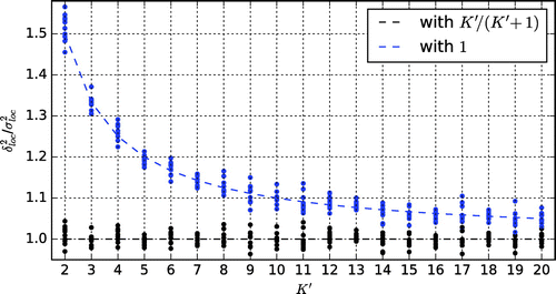The factor K′/(K′ + 1) on the right-hand side of Equation (20(20) $$E\left[\frac{1}{K^{\prime }-1}\sum _{k=1}^{K^{\prime }}{\left(d{\mathit{X}}^k-\overline{d\mathit{X}}\right)}^2\right]\left(t_f\right)=E\left[\frac{K^{\prime }}{K^{\prime }+1}{\overline{d\mathit{X}}}^2\right]\left(t_f\right).$$(20) ) may seem unusual, because in the ensemble forecasting literature the effects of sampling errors caused by the limited number of ensemble members on the spread–skill relationship is rarely considered. The omission of the normalization factor introduces only small errors into the estimate of the “skill” for the typical number (>20) of ensemble members (Fig. 2). What makes our situation special is that we allow for such small values of K′ as 2, for which the normalization factor is K′/(K′ + 1) = 2/3 ≈ 0.67, which is significantly smaller than 1.

Fig. 2. Illustration of the effect of the normalization factor K′/(K′ + 1) on the ratio of the estimates of the right- and left-hand sides of Equation (20(20) $$E\left[\frac{1}{K^{\prime }-1}\sum _{k=1}^{K^{\prime }}{\left(d{\mathit{X}}^k-\overline{d\mathit{X}}\right)}^2\right]\left(t_f\right)=E\left[\frac{K^{\prime }}{K^{\prime }+1}{\overline{d\mathit{X}}}^2\right]\left(t_f\right).$$(20) ).

Notes: The values shown are based on randomly generated samples of 10, 000 realizations of $\mathit{r}$, ${\mathit{r}}_a$, ${\mathit{r}}_f^k,k=1,\dots ,K^{\prime }$, assuming a Gaussian random distribution with mean $\overline{\mathit{r}}=\mathbf{0}$. Because of the sampling fluctuations, the simulation is repeated 10 times for each value of K′ and the results are shown by scatter-plots.

There is one additional issue that can affect the spread–skill relationship in the specific case of our morphing based verification technique, even if the ensemble correctly samples the true probability distribution: because the size of the search region limits the magnitude of the location error that the technique of Han and Szunyogh (2017) can detect, ${\mathit{r}}_f^k-\overline{{\mathit{r}}_f}$ and ${\mathit{r}}_a-\overline{{\mathit{r}}_f}$ is not always able to fully sample the tails of the probability distribution of the forecast uncertainty $\mathit{r}-\overline{\mathit{r}}$. This factor becomes important for the longer forecast times, at which ${\Sigma }_{\mathit{loc}}^2$ is typically large. The potential effects of this problem can be investigated by generating random samples of $\mathit{r}$, ${\mathit{r}}_a$ and ${\mathit{r}}_f^k$ for a prescribed value of ${\Sigma }_{\mathit{loc}}^2$ and then verifying the sample based estimates of ${\Sigma }_{\mathit{loc}}^2$ by ${\delta }_{\mathit{loc}}^2$ and ${\sigma }_{\mathit{loc}}^2$. 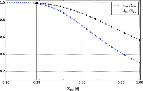Figure 3 summarizes the results of a simulation experiment along this line for an idealized, one-dimensional search domain (the position vectors are scalars along a line) of length 2d, assuming that ${\mathit{r}}_a$ is at the centre of the domain. The probability distribution of the location is assumed to be Gaussian, except that the tails of the distribution are truncated at plus and minus two standard deviations of the Gaussian distribution. The figure shows that once Σ_loc is larger than a critical value (about 0.29d), both σ_loc and δ_loc start to underestimate Σ_loc, but the magnitude of the estimation error grows faster for δ_loc than σ_loc as Σ_loc increases. We will make use of this finding in the analysis of the results on winter storms.

Fig. 3. The dependence of the prediction σ_loc and the estimate δ_loc on Σ_loc for a finite size search region.

Notes: The values shown are based on a randomly generated sample of 1000 realizations of $\mathit{r}$, ${\mathit{r}}_a$, ${\mathit{r}}_f^k,k=1,\dots ,100$, assuming a truncated Gaussian random distribution with mean $\overline{\mathit{r}}=\mathbf{0}$ in a one-dimensional search domain of size 2d. The values of Σ_loc on the x-axis are shown using the search radius d as unit, while the values of σ_loc and δ_loc on the y-axis are normalized by Σ_loc.

We have hitherto discussed the spread–skill relationship under the assumption that the ensemble sampled the true probability distribution of the forecast uncertainty of the location. To relax this assumption, it is important to first notice that the spread–skill relationship depends on the quality of the prediction of not only the variance, but also the mean of the probability distribution. In fact, as we have already discussed, sampling errors in the estimate of the mean have an effect on the spread–skill relationship. The other form of error in the prediction of the mean that we can account for in the spread–skill relationship is the forecast bias. In the presence of bias ${\mathit{\beta }}_{\mathit{loc}}\ne \mathbf{0}$, Equation (22(22) $${\delta }_{\mathit{loc}}^2\left(t_f\right)=\frac{1}{M^{\prime }\left(t_f\right)}\sum _{\begin{array}{c}m=1\\ K^{\prime }\left(m,t_f\right)\ge 2\end{array}}^M\left[\frac{K^{\prime }\left(m,t_f\right)}{K^{\prime }\left(m,t_f\right)+1}{\overline{d\mathit{X}}}^2\left(m,t_f\right)\right]$$(22) ) can be replaced by(23) $${\delta }_{\mathit{loc}}^2\left(t_f\right)=\frac{1}{M^{\prime }\left(t_f\right)}\sum _{\begin{array}{c}m=1\\ K^{\prime }\left(m,t_f\right)\ge 2\end{array}}^M\left[\frac{K^{\prime }\left(m,t_f\right)}{K^{\prime }\left(m,t_f\right)+1}{\overline{d\mathit{X}}}^2\left(m,t_f\right)\right]-{\left(\frac{1}{M^{\prime }\left(t_f\right)}\sum _{\begin{array}{c}m=1\\ K^{\prime }\left(m,t_f\right)\ge 2\end{array}}^M\left[\sqrt{\frac{K^{\prime }\left(m,t_f\right)}{K^{\prime }\left(m,t_f\right)+1}}\overline{d\mathit{X}}\left(m,t_f\right)\right]\right)}^2.$$(23)

This equation can be obtained by noticing that in the presence of bias, Equation (5(5) $$E\left[{\left({\mathit{b}}_{\mathit{loc}}\right)}^2\right]=E\left[{\left({\mathit{b}}_{\mathit{loc}}-E\left[{\mathit{b}}_{\mathit{loc}}\right]\right)}^2\right]=\frac{1}{K^{\prime }}{\mathrm{\Sigma }}_{\mathit{loc}}^2.$$(5) ) becomes(24) $$E\left[{\left({\mathit{b}}_{\mathit{loc}}\right)}^2\right]=E\left[{\left({\mathit{b}}_{\mathit{loc}}-E\left[{\mathit{b}}_{\mathit{loc}}\right]\right)}^2\right]=\frac{1}{K^{\prime }}{\mathrm{\Sigma }}_{\mathit{loc}}^2+E^2\left[{\mathit{b}}_{\mathit{loc}}\right],$$(24)

thus leading to the modified version(25) $$E\left[\frac{1}{K^{\prime }-1}\sum _{k=1}^{K^{\prime }}{\left(\overline{d\mathit{X}}-d{\mathit{X}}^k\right)}^2\right]\left(t_f\right)=E\left[\frac{K^{\prime }}{K^{\prime }+1}{\overline{d\mathit{X}}}^2\right]\left(t_f\right)-E^2\left[\sqrt{\frac{K^{\prime }}{K^{\prime }+1}}\overline{d\mathit{X}}\right]\left(t_f\right)$$(25)

of Equation (20(20) $$E\left[\frac{1}{K^{\prime }-1}\sum _{k=1}^{K^{\prime }}{\left(d{\mathit{X}}^k-\overline{d\mathit{X}}\right)}^2\right]\left(t_f\right)=E\left[\frac{K^{\prime }}{K^{\prime }+1}{\overline{d\mathit{X}}}^2\right]\left(t_f\right).$$(20) ). It is important to notice that Equation (23(23) $${\delta }_{\mathit{loc}}^2\left(t_f\right)=\frac{1}{M^{\prime }\left(t_f\right)}\sum _{\begin{array}{c}m=1\\ K^{\prime }\left(m,t_f\right)\ge 2\end{array}}^M\left[\frac{K^{\prime }\left(m,t_f\right)}{K^{\prime }\left(m,t_f\right)+1}{\overline{d\mathit{X}}}^2\left(m,t_f\right)\right]-{\left(\frac{1}{M^{\prime }\left(t_f\right)}\sum _{\begin{array}{c}m=1\\ K^{\prime }\left(m,t_f\right)\ge 2\end{array}}^M\left[\sqrt{\frac{K^{\prime }\left(m,t_f\right)}{K^{\prime }\left(m,t_f\right)+1}}\overline{d\mathit{X}}\left(m,t_f\right)\right]\right)}^2.$$(23) ) accounts only for the systematic part of the error in the prediction of the mean. Hence, flow dependent errors in the prediction of the mean can still lead to a breakdown of the modified spread–skill relationship (Equation 25(25) $$E\left[\frac{1}{K^{\prime }-1}\sum _{k=1}^{K^{\prime }}{\left(\overline{d\mathit{X}}-d{\mathit{X}}^k\right)}^2\right]\left(t_f\right)=E\left[\frac{K^{\prime }}{K^{\prime }+1}{\overline{d\mathit{X}}}^2\right]\left(t_f\right)-E^2\left[\sqrt{\frac{K^{\prime }}{K^{\prime }+1}}\overline{d\mathit{X}}\right]\left(t_f\right)$$(25) ).

2.3. Amplitude uncertainty

While the focus of the present paper is on the verification of the location forecasts, we also show verification results for the amplitude forecasts to contrast the behaviour of the diagnostics for the two forecast parameters. We describe the precipitation amount (amplitude) associated with a weather event by the areal mean μ of the precipitation in the verification domain, that is, by the ratio of the total precipitation in the verification domain and the area of the verification domain. Similar to the position $\mathit{r}$, we treat μ as a random variable. Let ${\mu }_f^k\left(m,t_f\right)$ $\left(k=1,2,\dots ,K^{\prime }\left(m,t_f\right)\right)$ be the areal mean of the precipitation in ensemble member k for forecast case m at forecast time t_f, and ${\mu }_a\left(m\right)$ the areal mean of the precipitation in the verifying analysis.

The bias $E\left[b_{\mathit{amp}}\right]$ of the areal mean precipitation (amplitude bias), which is the expected value of the difference(26) $$b_{\mathit{amp}}\left(m,t_f\right)=\overline{\mu }\left(m,t_f\right)-\overline{{\mu }_f}\left(m,t_f\right)$$(26)

between the mean $\overline{\mu }=E\left[\mu \right]$ and its ensemble-based prediction $\overline{{\mu }_f}$, can be estimated by(27) $${\beta }_{\mathit{amp}}\left(t_f\right)=\frac{1}{M^{\prime }\left(t_f\right)}\sum _{\begin{array}{c}m=1\\ K^{\prime }\left(m,t_f\right)\ge 2\end{array}}^M{b}_{\mathit{amp}}\left(m,t_f\right).$$(27)

In addition, by analogy to the arguments made earlier for the location uncertainty, the ensemble-based estimate of the amplitude uncertainty,(28) $${\sigma }_{\mathit{amp}}^2\left(t_f\right)=\frac{1}{M^{\prime }\left(t_f\right)}\sum _{\begin{array}{c}m=1\\ K^{\prime }\left(m,t_f\right)\ge 2\end{array}}^M\left[\frac{1}{K^{\prime }\left(m,t_f\right)-1}\sum _{k=1}^{K^{\prime }\left(m,t_f\right)}{\left({\mu }_f^k\left(m,t_f\right)-\overline{{\mu }_f}\left(m,t_f\right)\right)}^2\right],$$(28)

and the analysed uncertainty,(29) $${\delta }_{\mathit{amp}}^2\left(t_f\right)=\frac{1}{M^{\prime }\left(t_f\right)}\sum _{\begin{array}{c}m=1\\ K^{\prime }\left(m,t_f\right)\ge 2\end{array}}^M\left[\frac{K^{\prime }\left(m,t_f\right)}{K^{\prime }\left(m,t_f\right)+1}{\left({\mu }_a\left(m\right)-\overline{{\mu }_f}\left(m,t_f\right)\right)}^2\right],$$(29)

should be equal at any forecast time t_f.

3. Data

The diagnostics are applied to 0.5° × 0.5° resolution, global, 15-day long, twice daily, 20-member ensemble forecasts from the National Centers for Environmental Prediction (NCEP) of the US National Weather Service (NWS). The precipitation field at time t (e.g. 1200 UTC 2 January 2016) is defined by the accumulated precipitation for the 6-h period starting at time t. Because each of the 32 storms is present in multiple forecasts, the total number of verification cases considered is 133.

The search region for the estimation of the location error is 112 × 80 = 8960 grid points, which is about a region of 4900 km × 4400 km. The location of the search region is adjusted for each case such that the verifying precipitation feature is in the middle of the search region. Selecting a larger search region would eliminate the potential problem illustrated by Fig. 3, but the presence of multiple precipitation features in a larger search domain would also greatly complicate the implementation of the technique of Han and Szunyogh (2017).

The forecasts are verified against Stage IV precipitation analyses, which are based on radar and gauge observations over the US (Lin and Mitchell, 2005). These analyses are estimates of the rainfall accumulation for approximately 4 km × 4 km pixels. Since the precipitation system of winter storms often extends over the ocean, where no Stage IV data are available, we use 0.5° × 0.5° resolution, calibrated short-term (6-h) forecasts from the European Centre for Medium Range Forecasts (ECMWF) to fill the gaps in the verification data. Only those cases are included in the statistics for which more than 30% of the total precipitation in the verification region is associated with Stage IV data. The latter criterion reduces the number of forecast cases M from 133 to 83.

4. Results

4.1. The dependence of $K^{\prime }$ and $M^{\prime }$ on the forecast lead time

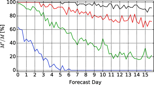
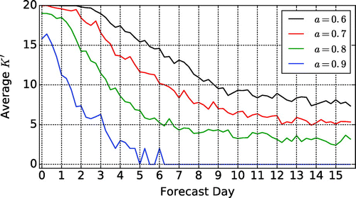
We start the examination of the results for the winter storms by an investigation of the typical number of ensemble members that predict the verifying storm. To be precise, we investigate the average of $K^{\prime }\left(m,t_f\right),m=1,2,\dots ,M$, over the M = 83 forecast cases (Fig. 4). As expected, the average K′ rapidly decreases with forecast time t_f. In addition, the decrease is more rapid for the larger values of a, that is, when a higher degree of similarity is required between the forecast and the verifying precipitation to declare that they are likely to be related. The saturation value of the curves in the figure also strongly depends on a. Because the saturation of the curves indicates that K′ no longer depends on the initial conditions, the saturation value of the ratio K′/K is an estimate of the likelihood that a storm is found sufficiently similar to the verifying storm by pure chance rather than due to forecast skill. This likelihood decreases with the increase of the required degree of similarity a between the forecast and the verifying precipitation event. In fact, the saturation value of K′/K can be reduced to zero by making the choice a = 0.9, but in that case, K′ < K even at initial time, which suggests that requiring such high degree of similarity between the forecast and the verifying precipitation field is unrealistic at the current level of modelling capabilities.

Fig. 4. Evolution of the average of K′ over all forecast cases for different values of a in the range from 0.6 to 0.9.

The decrease of the average of $K^{\prime }\left(m,t_f\right)$ with forecast time t_f suggests that $M^{\prime }\left(m,t_f\right)$ is also likely to decrease with the increase of t_f. This expectation is confirmed by the actual numbers (Fig. 5) that suggest that in order to maintain a sufficient sample size, a should be chosen not to be larger than a = 0.7. Because a = 0.7 is also the largest value of a for which K′ = K at analysis time (Fig. 4), we show the verification statistics for that particular value of a. We note, however, that we also carried out calculations for different values of a in the range from a = 0.6 to a = 0.9, and found that the verification results were robust to the choice of a, except for the presence of a higher level of noise for the larger values of a. We also note that Han and Szunyogh (2017) found the verification statistics to be similarly robust to the choice of a for deterministic forecasts.

Fig. 5. Evolution of the percentage M′/M of the forecast cases for which K′ ≥ 2 for different values of a in the range from 0.6 to 0.9.

4.2. Location bias and uncertainty

For the operational forecasts, both components of the estimated location bias are negligible for the first four forecast days (Fig. 6). After that, the magnitude of the zonal component gradually increases until saturation at about forecast lead time day 9–10 at a level of about – 300 km. The negative sign indicates that the eastward propagation of the storms is faster in the forecasts than reality. This result is consistent with the findings of Herrera et al. (2016) and Loeser et al. (2017) that the operational ensemble forecasts of the leading prediction centres of the world have a slowly developing bias that results in an overly zonal large scale flow (a flow that does not have a realistic south–north meandering large-scale component) at the longer lead times in the forecasts: because the large-scale flow acts as a guide for the eastward propagating storms, the overly zonal large-scale flow leads to an unrealistically fast eastward propagation of the storms and their precipitation systems. This slowly developing forecast bias is an indication of systematic model errors.

Fig. 6. Top: the values of $\overline{\mathit{dV}}$ for the individual ensemble forecasts (dark blue dots) and the evolution of the estimate of the meridional component of the location bias $E\left[{\mathit{b}}_{\mathit{loc}}\right]$ with the forecast lead time, bottom: the values of $\overline{\mathit{dU}}$ for the individual ensemble forecasts (dark blue dots) and the evolution of the estimate of the zonal component of the location bias $E\left[{\mathit{b}}_{\mathit{loc}}\right]$.

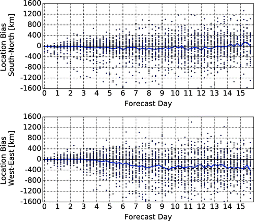
Figure 7 shows the functions ${\sigma }_{\mathit{loc}}\left(t_f\right)$, ${\delta }_{\mathit{loc}}\left(t_f\right)$, and ${\delta }_{\mathit{loc}}\left(t_f\right)$ after bias correction. There is a good agreement between ${\sigma }_{\mathit{loc}}\left(t_f\right)$ and the bias-corrected ${\delta }_{\mathit{loc}}\left(t_f\right)$ up to about 6 days. Beyond that, σ_loc becomes larger than both δ_loc and the bias corrected δ_loc, which indicates that the sampling problem illustrated in Fig. 3 does indeed affect the results. The general shape of the curves indicates a rapid chaotic growth of the forecast uncertainty before reaching saturation at about t_f = 11–14 days. This is the (absolute) predictability time limit for the location of the storms, the time beyond which no storm can be predicted with an accuracy higher than the accuracy of a forecast based on climatology. It should be noted that the predictability time limit for a specific storm can be significantly shorter than the absolute predictability time limit (e.g. Greybush et al., 2017).

Fig. 7. The evolution of σ_loc (solid black), δ_loc (solid blue) and bias-corrected δ_loc (dashed blue) with the forecast lead time.

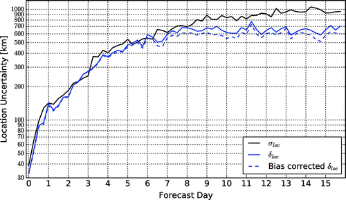
The saturation level of Σ, which is an estimate of the climatological value of the standard deviation of the distance between the locations of winter storms, can be estimated based on the results of Figs. 3 and 7. First, estimates of the saturation value of σ_loc, 1015 km, and the bias-corrected value of ${\delta }_{\mathit{loc}}\left(t_f\right)$, 626 km, can be obtained by a Lorenz-curve analysis (e.g. Han and Szunyogh, 2017). These estimates correspond to a ratio of 1015/626 = 1.62 of the values along the two curves in Fig. 3, which yields an estimate of Σ = 1530 km.

The information that the ratio between the saturation values of the diagnostics is 1.62 can also be used to obtain numerical estimates of the effective search radius d and the critical value 0.29d: the x-value that corresponds to the ratio of 1.62 in Fig. 3 is Σ = 0.81d, which combined with the estimate 1530 km of Σ leads to d = 1886 km and 0.29d = 550 km. Notice that the estimate of d is somewhat smaller than half of the length of the verification region in either direction. This relation between the search radius and the size of the verification region is due to the property of the verification region that it has to include the entire forecast precipitation feature for an accurate estimation of the location error.

The good agreement between the three curves in Fig. 7 for the first six forecast days suggests that the ensemble forecasts provide accurate quantitative prediction of the uncertainty of the location of the storms. Because the uncertainty in the location of the storms reflects uncertainty in the position of synoptic scale (∼1000 km) features of the atmospheric flow, our results indicate that the ensemble is highly efficient in capturing the uncertainty at the synoptic scales. As a counter-example to this behaviour, next we show that the ensemble is much less successful in capturing the uncertainty in the multi-scale processes that determine the precipitation amount. These processes take place in the range from micrometres in the clouds to thousands of kilometres at the synoptic scales.

4.3. Amplitude bias and uncertainty

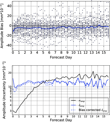
The evolution of the estimate of the amplitude bias β_amp (Fig. 8) indicates an initially rapidly and then slowly decreasing wet bias (over-prediction of the precipitation amount) in the forecasts, which completely disappears after about 13 days. The strong initial adjustment in the precipitation, which indicates that the model initial conditions are in the basin of attraction of the “attractor of the model dynamics”, but not exactly on the “attractor” (called “spin-up” in the numerical weather prediction jargon), has been a longstanding issue of numerical weather prediction. The fact that the wet bias eventually disappears as forecast time increases suggests that it is more likely to be due to problems with the initial conditions of the moist variables than systematic model errors. The relatively large initial value of ${\delta }_{\mathit{amp}}\left(t_f\right)$ also points to the initial conditions as the primary source of the amplitude forecast error in the first few forecast days. The ensemble spread ${\sigma }_{\mathit{amp}}\left(t_f\right)$, which predicts initially small and then rapidly growing amplitude errors, fails to capture the large initial errors, leading to an initially poor, but gradually improving ensemble performance. The fact that at the longer forecast lead times there is a much better general agreement between ${\sigma }_{\mathit{amp}}\left(t_f\right)$ and ${\delta }_{\mathit{amp}}\left(t_f\right)$ also supports the conclusion that the root of the initially large forecast errors and poor ensemble performance is primarily not a problem with the model climatology. This result calls for further research into the analysis and the generation of initial condition perturbations of moist model variables, for instance, by testing stochastic parameterization schemes and convective-allowing models in ensemble forecasting (e.g. Palmer et al., 2009; Khouider et al., 2010; Bengtsson and Körnich, 2016; Greybush et al., 2017).

Fig. 8. Top: the values of ${\mu }_a-\overline{{\mu }_f}$ for the individual ensemble forecasts (dark blue dots) and the evolution of the estimate of the amplitude bias $E\left[b_{\mathit{amp}}\right]$ with the forecast lead time, bottom: the evolution of σ_amp (solid black), δ_amp (solid blue) and bias-corrected δ_amp (dashed blue) with the forecast lead time.

5. Conclusions

In this paper, we introduced a morphing-based ensemble forecast verification technique for the location of precipitation events. We demonstrated the skill and the limitations of the technique with an application to operational ensemble forecasts of US winter storms. The results of this application suggest that the operational ensemble forecasts provide reliable forecasts of the uncertainty in the location of the storms, except for a slowly developing systematic error that leads to an unrealistically fast eastward propagation of the storms in the week-two forecasts. We contrasted the good performance of the ensemble in predicting the uncertainty in storm location to its poor performance in predicting the uncertainty of the precipitation amount in the short (less than 5 days) forecast range.

The most important limitation of the proposed verification technique in its present form is that it treats all precipitation in the verification region as part of single precipitation system. This makes the careful selection of the verification region a critical part of the implementation of the technique and it may lead to spurious results in situations where there are multiple, equally important, isolated features in the verification region (e.g. precipitation associated with multiple isolated convective systems). In light of these limitations, we view the current version of the technique as a highly useful research and development tool rather than a technique ready for an automated implementation for the routine verification of forecasts.

Disclosure statement

No potential conflict of interest was reported by the authors.

Funding

This work was supported by Climate Program Office [grant number NA16OAR4311082].

Acknowledgements

NCEP and ECMWF ensemble forecast data reported in the paper are archived in the TIGGE dataset (http://apps.ecmwf.int/datasets/data/tigge/). Stage IV analyses are available from https://data.eol.ucar.edu/dataset/21.093. This research has been conducted as part of the NOAA MAPP S2S Prediction Task Force and supported by NOAA grant NA16OAR4311082. Finally, we would like to thank the anonymous reviewers for their helpful comments.

Notes

1. While the practice of naming winter storms is controversial, the collection of named storms provides a representative sample of precipitation events that a major player of the US weather enterprise expected to have potentially high impact on society.

2. For instance, for an idealized precipitation field with a regular shape, $\mathit{r}$ could be defined by the centre of mass of the precipitation field. It should be noted, however, that for a complex precipitation field, the estimate of the location error by our technique is not necessarily equal to the error in the location of the centre of mass (Han and Szunyogh, 2016).

References

- Bengtsson, L. and Körnich, H. 2016. Impact of a stochastic parametrization of cumulus convection, using cellular automata, in a mesoscale ensemble prediction system. Q. J. Roy. Met. Soc. 142(695), 1150–1159.10.1002/qj.2016.142.issue-695
- Buizza, R. 1997. Potential forecast skill of ensemble prediction and spread and skill distribution of the ECMWF ensemble prediction system. Mon. Wea. Rev. 125, 99–119.10.1175/1520-0493(1997)125<0099:PFSOEP>2.0.CO;2
- Greybush, S. J., Saslo, S. and Grumm, R. 2017. Assessing the ensemble predictability of precipitation forecasts for the January 2015 and 2016 east coast winter storms. Wea. Forecasting 32(3), 1057–1078.10.1175/WAF-D-16-0153.1
- Han, F. and Szunyogh, I. 2016. A morphing-based technique for the verification of precipitation forecasts. Mon. Wea. Rev. 144, 295–313.10.1175/MWR-D-15-0172.1
- Han, F. and Szunyogh, I. 2017. A technique for the verification of precipitation forecasts and its application to a problem of predictability. Submitted to Mon. Wea. Rev. Preprint Online at: https://sites.google.com/a/tamu.edu/hanfan/.
- Herrera, M. A., Szunyogh, I. and Tribbia, J. 2016. Forecast uncertainty dynamics in the Thorpex Interactive Grand Global Ensemble (TIGGE). Mon. Wea. Rev. 144(7), 2739–2766.10.1175/MWR-D-15-0293.1
- Keil, C. and Craig, G. C. 2007. A displacement-based error measure applied in a regional ensemble forecasting system. Mon. Wea. Rev. 135, 3248–3259.10.1175/MWR3457.1
- Keil, C. and Craig, G. C. 2009. A displacement and amplitude score employing an optical flow technique. Wea. Forecasting 24, 1297–1308.10.1175/2009WAF2222247.1
- Khouider, B., Biello, J., Majda, A. J., et al. 2010. A stochastic multicloud model for tropical convection. Commun. Math. Sci. 8(1), 187–216.
- Lin, Y. and Mitchell K. E. 2005. The NCEP Stage II/IV hourly precipitation analyses: development and applications. In: 19th Conference of Hydrology, American Meteorological Society.
- Loeser, C. F., Herrera, M. A. and Szunyogh, I. 2017. An assessment of the performance of the operational global ensemble forecast systems in predicting the forecast uncertainty. Wea. Forecasting 32(1), 149–164.10.1175/WAF-D-16-0126.1
- Palmer, T., Buizza, R., Doblas-Reyes, F., Jung, T., Leutbecher, M., and co-authors 2009. Stochastic parametrization and model uncertainty. ECMWF Tech. Memo 598, 1–42.
- Talagrand, O., Vautard R. and Strauss B. 1999. Evaluation of probabilistic prediction systems. In: Proceedings of the ECMWF Workshop on Predictability, European Centre for Medium Range Weather Forecasts, Shinfield Park, Reading, Berkshire, UK, 1–25.
- Wang, Z. and Bovik, A. C. 2002. A universal image quality index. IEEE Signal Process. Lett. 9(3), 81–84. DOI:10.1109/97.995823.
- Wang, Z. and Bovik, A. C. 2009. Mean squared error: love it or leave it? A new look at signal fidelity measures. IEEE Signal Process. Mag. 26, 98–117.10.1109/MSP.2008.930649
- Wang, Z., Bovik, A. C., Sheikh, H. R. and Simoncelli, E. P. 2004. Image quality assessment: from error visibility to structural similarity. IEEE Trans. Image Process. 13, 600–612.10.1109/TIP.2003.819861
- Wernli, H., Paulat, M., Hagen, M. and Frei, C. 2008. SAL – a novel quality measure for the verification of quantitative precipitation forecasts. Mon. Wea. Rev. 136, 4470–4487.10.1175/2008MWR2415.1