Towards determining uncertainties in global oceanic mean values of heat, salt, and surface elevation

Abstract

Lower-bounds on uncertainties in oceanic data and a model are calculated for the 20-year time means and their temporal evolution for oceanic temperature, salinity, and sea surface height, during the data-dense interval 1994–2013. The essential step of separating stochastic from systematic or deterministic elements of the fields is explored by suppressing the globally correlated components of the fields. Justification lies in the physics and the brevity of a 20-year estimate relative to the full oceanic adjustment time, and the inferred near-linearity of response on short time intervals. Lower-bound uncertainties reflecting the only stochastic elements of the state estimate are then calculated from bootstrap estimates. Trends are estimated as $\text{2}\text{.2\hspace{0.17em}±\hspace{0.17em}0}\text{.2\hspace{0.17em}mm/y}$ in elevation, 0.0011 ±  0.0001 °C/y, and (−2.825 ± 0.17) × 10⁻⁵ for surface elevation, temperature and salt, with formal 2-standard deviation uncertainties. The temperature change corresponds to a 20-year average ocean heating rate of $0.48\pm 0.1$ W/m² of which 0.1 W/m² arises from the geothermal forcing. Systematic errors must be determined separately.

Keywords:

• elevation budgets
• global ocean heat
• model uncertainty
• salt
• uncertainty quantification

1. Introduction

Many papers have been directed at estimating multi-decadal ocean heat uptake (Purkey and Johnson, 2010; Lyman and Johnson, 2014), salinity change as an indicator of fresh-water injection (Wadhams and Munk, 2004; Boyer et al., 2005), and sea level (elevation) changes (Nerem et al., 2006; Cazenave et al., 2014) or all together (Levitus et al., 2005; Peltier 2009; Forget and Ponte, 2015). Many more such calculations have been published than can be listed here. A great difficulty with most of these estimates is the historical inhomogeneity in the various data sets employed, and the consequent assumption of nearly untestable statistical hypotheses used to extrapolate and interpolate into data sparse times and places (Boyer et al., 2016 and Wunsch, 2016 for generic discussions). A number of papers have claimed ‘closure’ of the sea level change budget, but that is accomplished through large and uncertain error budgets of the various components.

Ocean general circulation models (GCMs) and coupled climate models have also been used to calculate space- and time-mean oceanic temperature $(T),$ salinity $(S)$, and sea surface elevations $(\eta )$. Most models, including the ECCO system (Estimating the Circulation and Climate of the Ocean; Wunsch and Heimbach, 2013; Forget et al., 2015), compute the ocean state in a deterministic fashion. Given initial conditions and time-varying meteorological boundary conditions, the model time-steps the state vector$$, as though the external fields, including initial conditions, were fully known. Ensemble (Monte Carlo) methods attempt to estimate the uncertainties of the state at a particular time, usually a forecast time, by computing families of disturbed initial and/or boundary conditions.

A general discussion of the accuracy or precision of general circulation and climate models does not appear to exist. As in all systems, errors will always include systematic ones, e.g. from lack of adequate resolution or improperly represented air-sea transfer processes, amongst many others. Stochastic errors will arise from noisy initial and boundary conditions, as well as rounding errors, and interior instabilities of many types, both numerical and physical. Analysis of systematic and stochastic errors requires completely different methods. (Henrion and Fischoff, 1986, and especially their Fig. 1 reproduced in Wunsch 2015, p. 48.)

The central purpose of this paper is to suggest a potentially useful direction towards partially solving the problem of determining uncertainties in global-scale quantities calculated with both observations and models. Examples are produced for oceanic $T,S,\eta$ values and their variability from the nearly homogeneous (in the observational network sense) data sets 1994–2013. Specifically, a separation is attempted between the stochastic and systematic errors inevitably present. Stochastic errors are those often labeled as ‘formal’ and are derived from estimates of random noise present. Estimation of systematic errors involves a near line-by-line discussion of the individual computer codes used to calculate oceanic states. Errors will be different in calculations of the mean state, and in their temporal and spatial changes. For reasons discussed below, as the duration of a computation is extended, the distinction between stochastic and systematic errors can no longer be made and paradoxically, it is the comparatively short (20-year) time interval of the state estimate that supports the methodology outlined.

The ECCO version 4 solution employed here represents the output of an oceanic general circulation model whose initial and boundary (including meteorological) conditions and interior empirical coefficients have been adjusted in a least-squares sense to fit 25 years of global data. All data are assigned an error variance or covariance and the final state is obtained from the free-running adjusted system. For ‘state estimation’ as done in ECCO (Forget et al., 2015; ECCO Consortium 2017a,b; Fukumori et al., 2018), two major obstacles loom if Monte Carlo methods are to be used: (1) the immense state and control vector dimensions; (2) the absence of quantitative estimates (probability distributions) of the stochastic contributions in the initial/boundary conditions and stochastic structures generated by internal instability and turbulence. The same obstacles to uncertainty calculation loom in any ocean or coupled-climate model run for a long time whether or not based upon combinations with data.

A number of methods exist for calculating uncertainties in systems such as that of ECCO. To the extent that the system is linearizable, the method-of-Lagrange-multipliers/adjoint used there can be shown (Wunsch, 2006) to have identical uncertainties to those obtained from sequential estimates, such as the Rauch-Tung-Striebel (RTS) smoother.¹ This approach is very well understood and is practical for small systems (Goodwin and Sin, 1984; Brogan, 1991; Wunsch, 2006). It involves calculated covariance matrices that are square of the state vector dimension and of the control vector dimension at any time, t. For the ECCO version 4, state vector dimension at each time step is approximately N = 11 million and updating the state and its covariance requires running the model N + 1 times at each time-step. Similar dimensions and issues apply to the system control vector.

Other methods include calculation of inverse Hessians (Kalmikov and Heimbach, 2014), sometimes using Lanczos methods. Hypothetically, one could solve a Fokker–Planck equation corresponding to the model (Gardiner, 2004) and its initial/boundary condition, or the prediction-particle filtering methods of Majda and Harlim (2012). None of these methods is computationally practical for the global ocean or climate system with today’s computers – although that should gradually change in the future.

Nonetheless, some form of useful uncertainty estimate is necessary for values calculated from models, whether from ordinary forward calculations, or from a state estimate. For example, as described by ECCO Consortium (2017a), Fukumori et al. (2018), the 20-year average ocean temperature is 3.5310 °C found from the $N=2.4\times {10}^6$ volume weighted grid points of the adjusted model (centers of cells). How reliable is that number? On the one hand, it is extremely accurate up to the machine precision of $2^{-64}$. A standard error might be calculated by dividing the variance of the volume-weighted elements by $2.4\times {10}^6$, but such a number is meaningless: (1) much of the thermal structure of the ocean is deterministic on the large-scale – and with other effectively permanent sub-basin scale structures – stable over 20 + years. Treating that structure as stochastic would be a major distortion. (2) The distribution of values is very inhomogeneous over the three-dimensional volume and any supposition of uniform probability densities or of near-Gaussian values is incorrect.

Parts of the ocean structure and of the meteorological forcing fields are deterministic processes over decades. For example, the depth and properties of the main thermocline, or of the dominant wind systems, do not vary significantly over 20 years and the response times of the global ocean extend to thousands of years and beyond (Wunsch, 2015, p. 338). Superimposed upon the initial and boundary conditions are noise fields best regarded, in contrast, as stochastic – but which cannot build up global-scale covarying structures in a restricted time period.

When integrated through a time-stepping fluid model, the stochastic elements, even disturbances that are white noise in space and/or time, will give rise to complex structured fields (Fig. B5 of Wunsch, 2002). A crux of the uncertainty problem for model outputs then is to separate the deterministic from the stochastic elements. Ensemble methods, generated by stochastic perturbations of initial/boundary conditions/parameters, face the same difficulty: What are the appropriate joint probability distributions to use in generating the ensembles (Evensen, 2009)?² To the extent that the stochastic influence can be regarded as perturbations about a stable deterministic evolution, the probability densities will be centered about deterministic fields, as in Eq. (3.5.9) of Gardiner (2004). Systematic errors will remain as part of the deterministic components, and must be dealt with separately. A literature on systematic errors in numerical models does exist, much of it directed at the accuracies of advection schemes and other numerical approximations (Hecht et al., 1998). As is always the case with real systems, the stochastic error provides a lower bound on the true uncertainty.

What follows is largely heuristic and without any statistical rigor. Methods for separation of deterministic from stochastic elements in large volumes of numbers do not appear to have been widely explored. (This issue should not be confused with the problem of separating ‘deterministic chaos’ from true stochastic elements familiar in dynamical systems theory; Strogatz, 2015).

2. Mean values

A start is made with time-mean three-dimensional fields, which permits introducing the basic ideas while greatly reducing the volume of numbers required. A supposition is thus made that only the time average fields are available and sampled, temporarily suppressing the information contained in the time-variability. Suppression of the deterministic component, so as to leave a stochastic field, is required for both mean and time variations.

2.1. Temperature

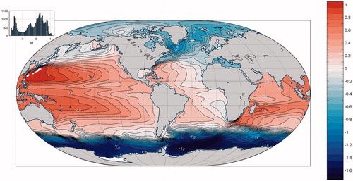
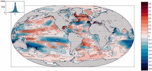
Consider the problem of determining the 20-year global ocean average temperature and its corresponding uncertainty. A 20-year average, computed 50 years in the future, might usefully be compared with the present 20-year average. Hourly values of the state estimate, averaged over 20-years, 1994–2013, produce point-wise calculated mean potential temperatures, ${\overline{T}}_i$ at each grid point. Mean temperature at one depth can be seen in Fig. 1, displaying the classical large-scale features that are clearly deterministic over 20 years with superimposed stochastic elements. A histogram of the gridded mean temperatures can be seen in Fig. 2 and its heavily skewed behavior is apparent.

Fig. 1. Twenty-year mean temperature at 105 m (°C). Inset shows the multi-modal histogram of values. The gyre structure is dominant and regarded here as a deterministic element of the field (Fukumori et al., 2018).

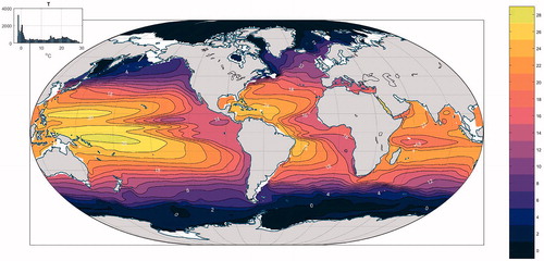
Fig. 2. (a) Histogram of temperature values occuring at each grid point in the 20-year average temperature. (b) Same as (a) except each value is weighted by the fractional volume corresponding to the particular grid point. (c) Variance with depth of the weighted temperatures in (b) before (solid line) and after (dashed line) removal of the lowest singular vector pair. (d) Cumulative sum of squared singular vectors for time-mean temperature field. (e) Histogram of values in the residual after removal of the q = 1 singular value pair and which is unimodal without a dominating skewness.

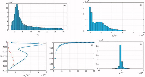
To form an average, the volume represented by each grid point is accounted for by weighting each value ${\overline{T}}_i$ by the relative volume contribution a_i such that, $$\tilde{m}={\displaystyle \sum _1^N{a}_i}{\overline{T}}_i=3.5310\pm ? °C,$$ as quoted above. A histogram of the similarly skewed weighted values can also be seen in Fig. 2. A standard deviation computed from the volume weighted values has no meaning as: (a) much of the field is effectively deterministic and, (b) the probability density of the stochastic elements is unknown.

Here the bootstrap and related jackknife methods in the elementary sense described by Efron and Tibsharani (1993), Mudelsee (2014), and others are used. The basic assumption of the bootstrap is that the values making up the subsampled population are independent, identically distributed (iid), values. Any assumptions that stochastic elements in cold, deep, temperatures are drawn from the same population as the much warmer near-surface values, or that this structure is dominantly stochastic, cannot be correct.

An assumption is now made that the strongest globally spatially varying structures represent the deterministic component. As already alluded to, this assumption is based on considerations of physics alone – and not upon any statistical methodology: any three-dimensional, globally correlated structure can only have been generated by very long-term effectively systematic processes. If a process can be rendered indistinguishable from white noise, then at zero-order most covariance structure has been removed.³ Integration of stochastic fields does, of course, produce globally correlated structures (Wunsch, 2002, Appendix B) but these take many decades and longer to appear. To the extent that the stochastic background has generated large-scale covarying fields, the results here will be biassed low. Experiments with simpler models (not shown) are supportive of the assumption that over time intervals, short compared to the full adjustment time of the system, stochastic disturbances can be so evaluated.

To render the assumption concrete, a residual population, ${\theta }_i^{\prime }={\left(a_i{\overline{T}}_i\right)}^{\prime },$ that is iid over the full water column everywhere is generated by subtracting the globally correlated structures. In particular, let the three-dimensional matrix of volume-weighted temperatures be, $\Xi \left({\lambda }_i,{\varphi }_j,z_k\right),$ written with columns in longitude, latitude, and depths. Setting temperatures to zero over land is the simplest choice. One might, alternatively, mask out these regions from the computation. Experiments (not shown) with the mean temperature field, showed only very slight differences from those obtained with the zero assumption (apart from weak structures appearing in the zero region, and masked out here). The choice has the virtue that the same method can be used in conjunction with coupled ocean-atmosphere models, where land values must be specified. Note too, that zeros are also assigned to regions below the local water depth so that the v_i vectors (defined below) can capture the influence of topography over a fixed interval of orthogonality.

To proceed, map this three-dimensional matrix $\Xi \left({\lambda }_i,{\varphi }_j,z_k\right)$ into two dimensions by stacking the latitude columns, to form ${\Xi }^{\prime }\left(r_{\alpha },z_k\right)$_, where $r_{\alpha }$ is just a reordering of longitude and latitude. Write ${\Xi }^{\prime }$ as its singular value decomposition, (1) $${\Xi }^{\prime }\left(r_{\alpha },z_k\right)=U_K{\Lambda }_K{V}_K^T,K\le 50,$$(1) where the vertical dimension is described by the K vectors, $v_i$, making up the columns of matrix $V_K.$ Columns of $U_k$ are denoted $u_i.$ K is the number of non-zero singular values and hence is the rank of ${\Xi }^{\prime }$. ($U_K,V_K$ contain the first K columns, etc. and ${\Lambda }_K$ is a K × K diagonal matrix.) The fractional value of the squared singular values, ${\lambda }_i=diag{({\Lambda }_K)}_i,$ as the sum, (2) $$S_{svd}(J)=\frac{{\displaystyle \sum _{j=1}^J{\lambda }_j^2}}{{\displaystyle \sum _{j=1}^K{\lambda }_{j^2}}}\le 1,J=1,\mathrm{\dots },K$$(2) is shown in Fig. 3 and representing the cumulative variance by singular vector pair. The first singular vector pair $u_1,v_1$ accounts for over 90% of the variance (Fukumori and Wunsch, 1991). A horizontal chart of $u_1$ is displayed in Fig. 3. Subtraction of q pairs, (3) $${\Xi }_q^{\prime }\left(r_{\alpha },z_k\right)={\Xi }^{\prime }-{\lambda }_1{u}_1{v}_1^T-{\lambda }_2{u}_2{v}_2^T-\mathrm{···}-{\lambda }_q{u}_q{v}_q^T={\displaystyle \sum _{j=q+1}^K{\lambda }_j}{u}_j{v}_j^T,$$(3) leaves a residual with a very much reduced spatially correlated structure. The variance with depth of both θ_i and ${\theta }_i^{\prime }$ (Fig. 2) shows that removal of the first pair alone ($q=1)$ leaves a variance much closer to being depth-independent and with a histogram that is unimodal and not heavily skewed, so that a standard deviation has some simple meaning. (A chart of $u_2,$ not shown, shows it to have a spatially complex structure with a plausibly stochastic behavior, which could be tested in turn.)

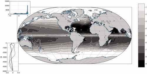
Fig. 3. Chart of the values of singular vector $u_1$ for volume weighted time mean temperatures $a_i{\overline{T}}_i$ as a function of position (multiplied by 1000). All contours shown are negative. Lower left inset displays (solid curve) the corresponding value with depth of $v_1$ (solid curve) along with $v_2$ (dashed) and $v_3$ (dotted). Note that $v_1\hspace{0.17em}<\hspace{0.17em}0$ almost everywhere so that the product, $u_1{v}_1^T$ is almost everywhere a positive volume weighted temperature. Upper left inset is the histogram of values and which is far from unimodal.

The crux of the statistical problem is in the decision about how many pairs, q, should be removed? A rigorous answer to this question is not provided here. Three basic criteria are used: (1) the residual should be unimodal; (2) the residual variance should not show a major depth dependence; (3) the dominant singular value should account for no less than 30% of the total variance. The criteria permit use of the estimated variance as a useful uncertainty parameter, and support for the iid assumption. A statistically rigorous result requires a method for use analogous to the use of the AIC (Akaike Information Criterion) or BIC (Bayesian Information Criterion) in linear regression analyses (Priestley, 1981).

For temperature, removal of only the first pair, $q=1,$ reduces the temperature norm of ${\Xi }_q^{\prime }\left(r_{\alpha },z_k\right)$ by over 90% and the histogram of volume weighted values (Fig. 2) is now unimodal. Over 20 years, the response of the ocean is dominantly linear, producing a normal stochastic field that is supported, e.g. by the discussion of Gebbie and Huybers (2018), and the known physics of short-time scale adjustment. With the risk of over-estimating the uncertainty, q = 1 is chosen, and the elements of ${\Xi }_q^{\prime }\left(r_{\alpha },z_k\right)$ are assumed to be iid and thus suitable for computing a bootstrap mean and standard error. Fifty samples of bootstrap reconstruction produces a two-standard deviation uncertainty of 1.9 × 10⁻³ °C owing to the stochastic elements or $〈T〉=3.531\pm 0.002$ °C, the ‘formal’ error. (For a Gaussian process, two-standard deviations is approximately 95% confidence interval.)

Much structure exists both in the suppressed and retained singular vector pairs, which ultimately need examination and physical explanation.

2.2. Salinity

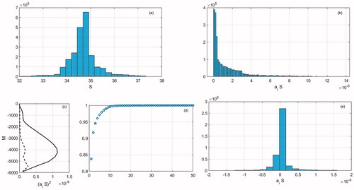
The time mean salinity, (34.727, dimensionless on the practical scale), determined from the volume-weighted values $a_i{¯S}_i$ has the histograms shown in Fig. 4.⁴ Taking now $q=2,$ $a_i{¯S}_i$, removes about 94% of the variance, and two standard deviations of the bootstrapped residual produces 34.72 ± 0.02. The variance with depth is rendered much more nearly uniform, albeit imperfectly so, and as for temperature, the residual histogram of $a_i{¯S}_i$ is now unimodal. That q = 2 for salinity rather than q = 1 for temperanture is likely explained by the much smaller deviations of S about its volumetric mean, but for present purposes that is immaterial.

Fig. 4. (a) Histogram of salinity values, ${\overline{S}}_i$ (dimensionless) on each model grid point. (b) Same as (a) except each salinity value is weighted by its corresponding fractional volume represented ($a_i{S}_i)$. (c) Variance of ($a_i{S}_i)$ with depth (solid curve) and after removing q = 2 pairs of singular vectors. (d) Normalized accumulating sum of singular values of $a_i{S}_i$. (e) Histogram of volume weighted residuals after removing q = 2 singular vector pairs.

For reference, under the assumption that total oceanic salt content remains unchanged, $\Delta h\hspace{0.17em}\approx -h_0\Delta S/S_0$ where h₀, S₀ are the mean values of mean depth and salinity (Munk, 2003) ignoring the density change to salinity⁵ and the contribution of melting sea ice, the uncertainty $\Delta S=\pm 0.02$ corresponds to a sea level change uncertainty of about $\Delta h=$ ± 2.2 m. This value may seem surprisingly large, but it simply says that the salinity data permits inference of the total amount of freshwater of about $\Delta h=2.2\text{\hspace{0.17em}m}$ out of a total average depth of about h = 3800 m, or about $0.06\%,$ which by most standards is remarkable accuracy. One can hope that a comparison 50 years hence will not find changes in $\Delta h$, which are significantly different from zero! The formal uncertainty in the present state is sufficiently small in determining systematic errors, care must be taken over the definition/calibration changes that may take place in the future as they have in the past; see Millero et al. (2008) for a discussion of systematic changes in definitions.

2.3. Sea surface height/dynamic topography

Mean sea surface height, $\eta ,$ the ‘dynamic topography’ in the present ocean state, can in principle be compared to its value determined as a 20-year average, 50 years, or any other time interval into the future. Values in the ECCO version 4 state estimate are determined relative to the best available geoid known today (Reigber et al., 2005). The dynamical variables are the horizontal gradient elements and thus if in the future, a different geoid is used, offset by a constant from the one used in ECCO, that change would be of no significance. On the other hand, care would be needed in the future to accommodate changed geoids, for example, with higher spatial resolution, temporal changes, and with significant regional implications. Because dynamics respond only to horizontal gradients in $\eta ,$ the result is most directly connected to the altimeter, gravity, and hydrographic data.

The assumption used so far, that globally covarying fields over 20 years can be interpreted as the deterministic components, is physically sensible for temperature and salinity. For η, however, the ability of the ocean to transmit barotropic (depth independent) signals globally within a few days, makes the assumption dubious. Nonetheless, with this caveat, the global time-mean value of η and an estimate of its accuracy is calculated within the model context. Because of the complexities of geoid error and the rapid achievement of barotropic motion equilibrium, only the time differences of the mean surface height are discussed. For the record, the area weighted mean of the values in Fig. 5 is 8.48 ± 0.13 cm with the error based upon $q=3,$ but no more discussion is provided here.

Fig. 5. Time mean elevation (dynamic height) corrected for ice cover weight (Fukumori et al. 2018). Values are multimodal.

3. Time changes: difference of last and first years

Time changes, represented for now by the difference between two yearly-averages, years t₁, t₂, should largely remove the deterministic components contained in the initial/boundary conditions. A trend, e.g. in exchange of heat between ocean and atmosphere as a part of the global warming signal and part of the surface boundary conditions, might be regarded as deterministic. But, as has been noted in numerous publications (Ocaña et al., 2016), with a 20-year record, the duration is far too short to distinguish a true deterministic trend from the long-term stochastic shifts characteristic of red-noise processes. Thus, any trend present is treated as though arising from a stochastic process. Discussion of temporal changes is done in two ways: (1) the value of the differences of the first and last years (20-year difference), and which makes no assumptions about the nature of the trend. (2) The bootstrapped or jackknifed estimate of the trends, assumed to be linear ones using all of the intermediate year averages.

3.1. Temperature/heat content

One interesting example is the difference between the mean ocean temperature in 2013 and what it was in 1994 (shown for two depths in Figs. 6–7) – as a constraint on the rates of global warming. This difference is again a static field and can be analyzed in the same fashion as the time-mean was treated. The spatial pattern of warming and cooling is a complicated one with large-scale structures corresponding to known physical regimes, e.g. the eastern tropical Pacific, the near-Gulf Stream system/subpolar gyre, the Southern Ocean. As one might expect, temperature difference variances are much larger near the surface than they are in the abyss and the gridded temperature field itself is far from having an iid. One can proceed as above, subtracting the appropriate three-dimensional singular vector pairs. To shorten the discussion, the temperature differences are here integrated in the vertical to different depths, including the bottom. The top-to-bottom area-weighted integrals and their histogram distribution are shown in Fig. 8.

Fig. 6. Temperature difference at 105 m between 2013 and 1994 (°C). Values are unimodal.

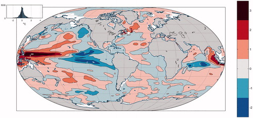
Fig. 7. Temperature difference (^oC) at 1000 m between 2013 and 1994.

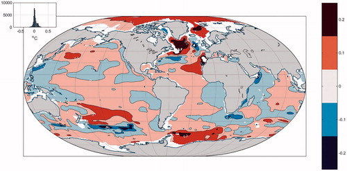
Fig. 8. Vertical integral, top-to-bottom, of the temperature difference between 2014 and 1993 and area weighted (106 °C). The result is treated as fully stochastic, which may somewhat overestimate the formal uncertainty ($q=0)$. Histogram is again unimodal. Spatial complexity here is indicative of the difficult oceanic sampling problem.

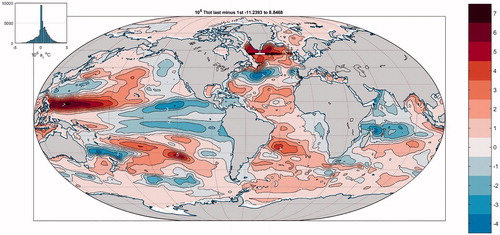
Note that the two yearly estimates are not independent ones – they are connected through the time-evolving equations of motion. To the extent that any systematic error in the ECCO system is time-independent, it will be subtractive in the time-difference. The vertical integral, top-to-bottom has no dominant singular vector pair, with the largest squared singular value accounting for less than 30% of the variance. Proceeding under the assumption that the 20-year time-difference has a vertical integral that is close to iid ($q=0)$, the bootstrap produces a temperature change of $\left(0.0206\hspace{0.17em}\pm \hspace{0.17em}6.7\right)\times {10}^{-4}$ °C (two standard deviations). The underlying ECCO GCM uses a constant heat capacity of $c_p=\text{3994\hspace{0.17em}J}/°\text{C}/\text{kg}$, so that with an ocean mass of $1.37\times {10}^{21}\text{\hspace{0.17em}kg},0.0\text{2}$ °C corresponds to a net heat change of $(1.1\hspace{0.17em}\pm \hspace{0.17em}0.37)\times {10}^{23}\text{\hspace{0.17em}J}$. Over 20 years, the heating rate is approximately 0.48 ± 0.16 W/m² including 0.095 W/m² from geothermal heating (ECCO Consortium, 2017a). As a rough comparison, Levitus et al. (2012), estimated a change of $\left(2.4\hspace{0.17em}\pm \hspace{0.17em}0.19\right)\times {10}^{23}\text{\hspace{0.17em}J}$, but to 2000 m and in the interval 1955–2010 for a rate of 0.4 W/m², and using an entirely different basis for the uncertainty estimate.

With all the results here, these values represent lower bounds on the uncertainty. Geothermal heating itself has uncertainties, which should be separately analyzed, and the dependence of heat capacity and density on temperature, salinity, and pressure will introduce systematic errors.

3.2. Salinity/freshwater

The pattern of vertically integrated differences of salinity between 1994 and 2013 (Fig. 9) is already visually somewhat stochastic in character and thus no further structure is removed (the largest singular value corresponds to only 20% of the variance). The mean salinity change between the two years is (−5.4 ± 0.84) × 10⁻⁴ from the bootstrap estimate with q = 0. Using the above expression for the addition of freshwater, the net increase in water depth is $0.0\text{6\hspace{0.17em}}\pm \mathrm{\hspace{0.17em}0.01}\text{\hspace{0.17em}m}$, or 3.0 ± 0.5 mm/y.

Fig. 9. Vertically integrated salinity difference 2013–1994, top-to-bottom.

3.3. Surface height

The difference in height over 20 years (Fig. 10) is 6.37 ± 0.3 cm, or an average change of 3.2 ± 0.015 mm/y where the standard error is obtained from the bootstrap with $q=2.$ Nerem et al. (2006) quote a rate from altimeter data alone, as 3.1 ± 0.4 mm/y. Although the estimates are not independent – the state estimate uses all the altimeter data – and the altimeter data do not extend over the ice-covered region – the results are approximately consistent. (See Lanzante, 2005, for the interpretation of overlapping uncertainty estimates.)

Fig. 10. Annual mean anomaly of surface elevation (m) relative to the 20-year mean in Fig. 5 over 20 years (upper panel). Error estimates are from a bootstrap of the spatial distribution of the anomaly field in each year, with q = 0. Lower panel shows the simple year-to-year difference of the values in the upper panel with the uncertainty estimates between each year treated as independent.

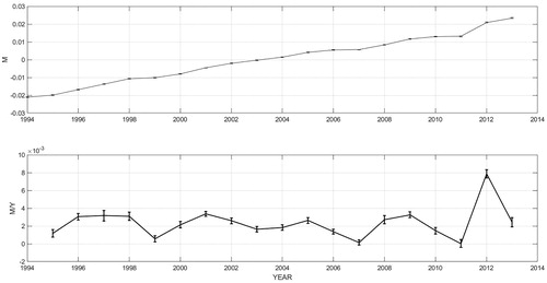
η is calculated in the model using the full equation of state, thus accounting for the addition of freshwater, the thermal expansion from external heating, and any interior redistribution of heat and salt as functions of position and depth. The change in elevation over 20 years of 6.4 ± 0.3 cm is crudely then about 5–6 cm from the addition of freshwater, with any remainder attributable to thermal expansion.

4. Estimated linear trends

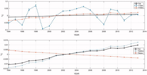
A generalization for both temperature and salinity is that the top 100 m are noisy year-to-year, but that integrals to 700 m are much cleaner and visually very close to linear. In both fields, the abyssal region, defined as the levels below 3600 m, shows a counter-trend to that of the water-column total.

4.1. Temperature/heat content

The integrated temperature to various depths is shown in Fig. 11. The best fitting, assumed linear, trend over 20 years is sought, whether deterministic or a red-noise random walk is immaterial at this stage. The least-squares fit mean slope for the top-to-bottom change is $0.0011\hspace{0.17em}\pm \hspace{0.17em}6.9\times {10}^{-5}$ °C/y. Standard error is computed from a bootstrap of the full field, under the assumption that the time differences are basically stochastic – and which likely slightly overestimates the uncertainty. (A jackknife estimate was identical.) The mean slope implies a change over 20 years of 0.0213 ± 0.0014 °C and which differs only slightly from the value computed between first and last years as might have been inferred from Fig. 11.

Fig. 11. Annual mean temperature anomalies integrated to different depths including the bottom in °C. Two standard deviation bars are derived from bootstrapping the full temperature difference field each year. Ttot is integrated top-to-bottom; T100m, T700m, T3600m are integrated to 100, 700, and 3600 m, respectively. Tabyss is integrated from 3600 m to the bottom. Cooling in the region below 3600 m was discussed by Wunsch and Heimbach (2014) and Gebbie and Huybers (2018).

4.2. Salinity trends

Integrated salt anomalies are displayed for each year to several depths in Fig. 12. An overall freshening, top-to-bottom is evident, including a slight increase in salinity at and below 3600 m. This abyssal change accompanies the general cooling seen below 3600 m in Fig. 11, but this physics is not further described here.

Fig. 12. Same as Fig. 9, except for the mean vertically integrated salinity anomaly (practical scale) for each year with an estimated 2-standard deviation error bar. Total is repeated in both panels. Note overall freshening, with a partly compensating increase in salinity in the abyss. A best-fitting linear trend for the total change is discussed in the text.

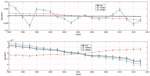
As with temperature, the best fitting least-squares straight line differs slightly from the calculation using only the first and last years, producing a value of $\left(-2.825\pm 0.137\right)\times {10}^{-5}/\text{y}$ for a net change over 20 years of $\left(-5.65\hspace{0.17em}\pm \hspace{0.17em}0.274\right)\times {10}^{-4}$ (For comparison, Boyer et al., 2005, estimated the trend as $-5.4\times {10}^{-4}/\text{y}$ from a much longer and much more inhomogeneous data set. No uncertainty was specified.)

4.3. η Trends

Fig. 10 displays the annual spatial average anomaly values of η and the first differences in each year. The spatial patterns do not show a single dominant singular value (10 of them are required to account for 90% of the variance).

An estimate of the trend is $2.2\times {10}^{-3}\pm 1.5\times {10}^{-4}\text{\hspace{0.17em}m/y}$, again from a bootstrap average (with $q=0$), of about 2 mm/y. The corresponding mean surface height change is then 4.4 ± 0.15 cm over the 20 years. Attribution of the combined heating and salinity change into an equivalent sea level trend is a complex matter, that must include gravity field changes (see Church et al. 2010; Pugh and Woodworth 2014; and Forget and Ponte 2015) for complete discussion.

5. Discussion

Although quantitative 20-year time-means and changes in the global average oceanic heat, salt, and dynamic topography (sea surface height) have been estimated, the main goal here is not those numbers per se: the intention is to begin the discussion of the separation of random and systematic errors in model property estimates. Results here are almost entirely heuristic, but the approach using resampling (bootstrap) methods applied to spatially decorrelated fields can perhaps be made rigorous. In particular, methods for separating deterministic and stochastic elements of the three-dimensional, time-dependent fields, in the absence of real knowledge of the probability distributions, should be explored. Formal errors here are sufficiently small that a reasonable expectation is that systematic ones dominate, but that is only surmise. Attention must then turn to the issue of systematic errors in the model and state estimate. These will never be zero, but because of the data-fitting in the state estimation process, they are expected to be much-reduced compared to those found in unadjusted climate models.

A full discussion of the structures and causes of the various fields appearing in the means and in the heating/cooling, salinification/freshening, elevation increases/decreases in time and space requires a specialized study of each field separately and is not attempted here.

Acknowledgments

G. Gebbie and D. Amrhein had useful comments on an early version. Suggestions from the anonymous reviewers also proved helpful.

Disclosure statement

No potential conflict of interest was reported by the author.

Notes

Additional information

Funding

This work was supported by the National Aeronautics and Space Administration through an MIT contract with JPL.

Notes

1 The RTS smoother employs the Kalman filter as a sub-component in the numerical algorithm. Kalman filters are predictors and should not be confused with general smoothing estimators. In any case, true Kalman filters, which require continual updating of the covariance matrices, are never used with realistic large-scale fluid problems – the dimensionality is overwhelming. In practice, the prediction numerics are usually approximated forms of Wiener filters, which employ temporally fixed, guessed, covariances.

2 Computationally practical ensemble dimensions remain orders of magnitude smaller than any reasonable estimate of the number of degrees-of-freedom.

3 An alternative, not used here, would be a spectral expansion in spherical harmonics and a choice of vertical basis functions, and the exploitation of the non-random character of the coefficients of the deterministic elements.

4 Worthington’s (1981) value for temperature was 3.51 °C and for salinity was 34.72 g/kg on the older salinity scale, again with no stated uncertainty. Both are very close to the present estimated values, although pertaining to the historical period prior to about 1977.

5 The 20-year difference in global mean density is ≈−0.0038 kg/m³ including the thermal and salinity effects.

References

- Boyer, T., Domingues, C. M., Good, S. A., Johnson, G. C., Lyman, J. M. and co-authors. 2016. Sensitivity of global upper-ocean heat content estimates to mapping methods, XBT bias corrections, and baseline climatologies. J. Clim. 29(13), 4817–4842.
- Boyer, T. P., Levitus, S., Antonov, J. I., Locarnini, R. A. and Garcia H. E. 2005. Linear trends in salinity for the World Ocean, 1955–1998. Geophys. Res. Lett. 32(1), L01604.
- Brogan, W. 1991. Modern Control Theory. 3rd Ed. Prentice-Hall, Englewood Cliffs, NJ.
- Cazenave, A., Dieng, H.-B., Meyssignac, B., Von Schuckmann, K., Decharme, S. and co-authors. 2014. The rate of sea-level rise. Nature Clim. Change. 4, 358–361. DOI:10.1038/nclimate2159.
- Church, J. A., Woodworth, P. L., Aarup, T. and Wilson, W. S. 2010. Understanding Sea-Level Rise and Variability. Wiley-Blackwell, Chichester, West Sussex; Hoboken, NJ, pp. 428.
- ECCO Consortium. 2017a. A twenty-year dynamical oceanic climatology: 1994–2013. Part 1: Active scalar fields: temperature, salinity, dynamic topography, mixed-layer depth, bottom pressure. MIT DSpace. Online at: http://hdl.handle.net/1721.1/107613
- ECCO Consortium. 2017b. A twenty-year dynamical oceanic climatology: 1994–2013. Part 2: Velocities and property transports. MIT DSpace. Online at: http://hdl.handle.net/1721.1/109847
- Efron, B. and Tibshirani R. 1993. An Introduction to the Bootstrap. Chapman & Hall, New York.
- Evensen, G. 2009. Data Assimilation: The Ensemble Kalman Filter. Springer Verlag, Berlin.
- Forget, G., Campin, J. -M., Heimbach, P., Hill, C., Ponte R. and co-authors. 2015. ECCO version 4: an integrated framework for non-linear inverse modeling and global ocean state estimation. Geosci. Model Dev. 8, 3071–3104.
- Forget, G. and Ponte, R. M. 2015. The partition of regional sea level variability. Prog. Oceanogr. 137, 173–195.
- Fukumori, I., Heimbach, P., Ponte R. M. and C. Wunsch. 2018. A dynamically-consistent ocean climatology and its temporal variations. Bull. Am. Met. Soc., in press.
- Fukumori, I. and Wunsch, C. 1991. Efficient representation of the North Atlantic hydrographic and chemical distributions. Prog. in Oceanog. 27, 111–195.
- Gardiner, C. W. 2004. Handbook of Stochastic Methods for Physics, Chemistry, and the Natural Sciences. 3rd Ed. Springer-Verlag, Berlin.
- Gebbie, G. and Huybers, P. 2018. The Little Ice Age and 20th-century deep Pacific cooling. Submitted for publication.
- Goodwin, G. C. and Sin, K. S. 1984. Adaptive Filtering Prediction and Control. Prentice-Hall, Englewood Cliffs, NJ.
- Hecht, M. W., Bryan, F. O. and Holland, W. R. 1998. A consideration of tracer advection schemes in a primitive equation ocean model. J. Geophys. Res. -Oceans. 103, 33301–3321.
- Henrion, M. and Fischhoff, B. 1986. Assessing uncertainty in physical constants. Am. J. Phys. 54(9), 791–798.
- Kalmikov, A. and Heimbach, P. 2014. A Hessian-based method for uncertainty quantification in global ocean state estimation. SIAM J. Sci. Comput. 36(5), S267–S295.
- Lanzante, J. R. 2005. A cautionary note on the use of error bars. J. Climate. 18, 3669–3703.
- Levitus, S., Antonov, J. I., Boyer, T. P., Garcia, H. E. and Locarnini, R. A. 2005. Linear trends of zonally averaged thermosteric, halosteric, and total steric sea level for individual ocean basins and the world ocean, (1955–1959)–(1994–1998). Geophys. Res. Lett. 32(16), L16601. DOI:10.1029/2005gl023761.
- Levitus, S., Antonov, J. I., Boyer, T. P., Baranova, O. K. and co-authors. 2012. World ocean heat content and thermosteric sea level change (0-2000 m), 1955–2010. Geophys. Res. Letts. 39. DOI:10.1029/2012gl051106.
- Lyman, J. M. and Johnson, G. C. 2014. Estimating global ocean heat content changes in the Upper 1800 m since 1950 and the influence of climatology choice. J. Clim. 27(5), 1945–1957.
- Majda, A. J. and Harlim, J. 2012. Filtering Complex Turbulent Systems. Cambridge University Press, Cambridge.
- Millero, F. J., Feistel, R., Wright, D. G. and McDougall, T. J. 2008. The composition of standard seawater and the definition of the Reference-Composition Salinity Scale. Deep Sea Res. Part I Oceanogr. Res. Pap. 55(1), 50–72.
- Mudelsee, M. 2014. Climate Time Series Analysis: Classical Statistical and Bootstrap Methods. Springer, Dordrecht.
- Munk, W. 2003. Ocean freshening, sea level rising. Science. 300(5628), 2041–2043.
- Nerem, R. S., Leuliette, E. and Cazenave, A. 2006. Present-day sea-level change: a review. Comptes Rendus Geoscience. 338(14–15), 1077–1083.
- Ocaña, V., Zorita, E. and Heimbach, P. 2016. Stochastic trends in sea level rise. J. Geophys. Res. 121. DOI:10.1002/2015JC011301.
- Peltier, W. R. 2009. Closure of the budget of global sea level rise over the GRACE era: the importance and magnitudes of the required corrections for global glacial isostatic adjustment. Quat. Sci. Rev. 28(17–18), 1658–1674.
- Priestley, M. B. 1981. Spectral Analysis and Time Series. Vol 2, pp. 890. Academic, London.
- Pugh, D. and Woodworth, P. L. 2014. Sea-Level Science: Understanding Tides, Surges, Tsunamis and Mean Sea-Level Changes. Cambridge University Press, Cambridge, pp. 395.
- Purkey, S. G. and Johnson, G. C. (2010). Warming of global abyssal and deep southern ocean waters between the 1990s and 2000s: contributions to global heat and sea level rise budgets. J. Clim. 23(23), 6336–6351.
- Reigber, C., Schmidt, R., Flechtner, F., Konig, R., Meyer, U. and co-authors. 2005. An earth gravity field model complete to degree and order 150 from GRACE: EIGEN-GRACE02S. J. Geodyn.. 39(1), 1–10.
- Strogatz, S. H. 2015. Nonlinear Dynamics and Chaos: With Applications to Physics, Biology, Chemistry, and Engineering. Westview Press, Boulder, CO.
- Wadhams, P. and Munk, W. 2004. Ocean feshening, sea level rising, sea ice melting. Geophys. Res. Lett. 31, L11311. DOI:10.1029/2004gl020039.
- Worthington, L. V. 1981. The water masses of the world ocean: some results of a fine-scale census. In: Evolution of Physical Oceanography. Scientific Surveys in Honor of Henry Stommel (eds. B. A. Warren and C. Wunsch), The MIT Press, Cambridge, pp. 42–69. Online at: http://ocw.mit.edu/ans7870/textbooks/Wunsch/wunschtext.htm
- Wunsch, C. 2002. Oceanic age and transient tracers: analytical and numerical solutions. J. Geophys. Res. 107(C6), L304810. DOI:1029/2001jc000797.
- Wunsch, C. 2006. Discrete Inverse and State Estimation Problems: With Geophysical Fluid Applications. Cambridge University Press, Cambridge, New York.
- Wunsch, C. 2015. Modern Observational Physical Oceanography. Princeton University Press, Princeton.
- Wunsch, C. 2016. Global ocean integrals and means, with trend implications. Annu. Rev. Mar. Sci. 8, 1–33.
- Wunsch, C. and Heimbach, P. 2013. Dynamically and kinematically consistent global ocean circulation state estimates with land and sea ice. 2nd Ed. In: Ocean Circulation and Climate, (eds. J. C. G. Siedler, W. J. Gould, and S. M. Griffies), Elsevier, Amsterdam, pp. 553–579.
- Wunsch, C. and Heimbach, P. 2014. Bidecadal thermal changes in the abyssal ocean and the observational challenge. J. Phys. Oc. 44, 2013–2030.