Recent subsurface North Atlantic cooling trend in context of Atlantic decadal-to-multidecadal variability

Abstract

The spatiotemporal structure of the recent decadal subsurface cooling trend in the North Atlantic Ocean is analyzed in the context of the phase reversal of Atlantic multidecadal variability. A vertically integrated ocean heat content (HC) Atlantic Multidecadal Oscillation index (AMO-HC) definition is proposed in order to capture the thermal state of the ocean and not just that of the surface as in the canonical AMO SST-based indices. The AMO-HC (5–657 m) index (defined over the area, 0°N–60°N, 5°W–75°W) indicates that: (1) The traditional surface AMO index lags the heat content (and subsurface temperatures) with the leading time being latitude-dependent. (2) The North Atlantic subsurface was in a warming trend since the mid-1980s to the mid-2000s, a feature that was also present at the surface with a lag of 3 years. (3) The North Atlantic subsurface is in a cooling trend since the mid-2000s with significant implications for predicting future North Atlantic climate. The spatial structure of decadal trends in upper-ocean heat content (5–657 m) in the North Atlantic prior to and after 2006 suggests a link with variability of the Gulf Stream–Subpolar Gyre system. The Gulf Stream leads variability in upper-ocean heat content over the Subpolar region by ∼13 years, and the lead increases from east to west from the Iceland Basin to the Irminger Sea to the Labrador Sea. The similarity between the structure of decadal mean anomalies, their change and trends in upper-ocean heat content and salinity in the North Atlantic and anomalies associated with a Gulf Stream index is striking. In this scheme, the displacements of the Gulf Stream–North Atlantic Current systems and their interactions with the Subpolar Gyre, as part of the meridional overturning circulation, have a decisive role for imposing decadal variability in both the Ocean and hydroclimate over the neighbouring continents.

Keywords:

• Gulf Stream
• subpolar gyre
• Atlantic multidecadal variability
• recent cooling trend
• decadal variability

1. Introduction

The state of the North Atlantic Ocean is a key element in understanding regional and global climate variability and change. Reversals of SST anomalies over the North Atlantic have decadal-to-multidecadal variability, which, in turn, imposes warming and cooling decadal trends when transitioning from one phase to the other. Basin-wide trends have traditionally been identified via the Atlantic Multidecadal Oscillation (AMO) index (Enfield et al., 2001; Guan and Nigam, 2009), an SST-based index which integrates the vagaries of the atmosphere and as such tends toward the low-frequencies (e.g. Frankignoul and Hasselmann, 1977; Deser et al., 2010). However, the characteristic features of the Subpolar Gyre (SPG) and Subtropical Gyre, warm and cold currents (Reverdin et al. 2003), including the Gulf Stream (GS) system, and their advective properties make the region more than a passive responder to atmospheric variability (Bjerknes, 1964; Bryan and Stouffer, 1991; Wang et al., 2004; Reverdin, 2010; Zhang et al., 2016; Delworth et al., 2017; Zhang, 2017; Nigam et al., 2018).

Modelling and empirical analyses indicate that heat transports by the Gulf Stream–North Atlantic Current (GS–NAC) system are important in order to have low-frequency variability in the North Atlantic (Sutton and Allen, 1997; Delworth et al., 2017; Zhang, 2017). Atlantic multidecadal variability requires these transports to be properly accounted for (Drews and Greatbatch, 2016). Not surprisingly the largest year-to-decadal variability occurs along this current system (Buckley and Marshall, 2016). Extreme climate episodes in the North Atlantic at decadal scales are characterized by an out-of-phase relationship of the oceanic conditions between the Subpolar Gyre and GS regions (Häkkinen, 2001; Zhang, 2008; Häkkinen and Rhines, 2009; Häkkinen et al., 2013; Zhang and Zhang, 2015). As such, cooling trends in the upper North Atlantic Ocean such as those after the 1970s (Rahmstorf et al., 2015) and after 2005 have recently been related to a weakening of the Atlantic Meridional Overturning Circulation (AMOC) by Robson et al. (2016). The latter investigators found that the density anomalies became negative due to the pronounced 1995–2005 warming of the subpolar gyre, which, in turn, decreased the strength of the formation of North Atlantic deep waters and ultimately lead to a negative anomaly in the meridional heat transport and hence a cooling. This buoyancy-driven AMOC response is likely to also have triggered the cooling of the 1960s (Robson et al., 2014). Most importantly, Robson et al. (2016) concluded by examining trends in atmosphere–ocean surface fluxes and SSTs that the warming and cooling trends observed before and after 2005 were of oceanic rather than of atmospheric nature. There is, however, yet much to learn not only about this newly reported decadal cooling trend of the Subpolar North Atlantic (SPNA) but also about how regional decadal trends are produced, regarding the role of propagating subsurface anomalies as well as their link with the GS, North Atlantic current (NAC) and SPG system.

In the present paper, the surface and subsurface thermal structures of the North Atlantic basin, especially its decadal-to-multidecadal variability are closely examined to provide some insights on the role of the GS–NAC–SPG system in the generation of the recent decadal cooling. The thermal state of the North Atlantic surface waters is characterized here by using the areal average of the seasonal SST anomalies in the 75°W–5°W and Eq–60°N domain, viz. the AMO index. This index is, typically, linearly detrended and smoothed to highlight decadal–multidecadal variability; the spatiotemporal evolution of the AMO, identified as a mode of SST variability in the Atlantic, was characterized in Guan and Nigam (2009), and its subsurface structure explored in Kavvada et al. (2013). There is an interplay in upper-ocean heat content anomalies between the SPG and GS regions which changes with time before and after the mature phase. In particular, under the mature positive phase of the AMO, the subpolar region warms while the GS path region, along the North American coast, cools (Fig. 7 in Kavvada et al., 2013; Wang and Zhang, 2013; Zhang and Zhang, 2015). Similarly to the surface AMO index, and following Kavvada (2014), the subsurface thermal state is characterized using the same areal averaging but of linearly detrended ocean heat content (HC) over various column depths; hereafter, the AMO-HC index. The ocean heat content is an informative variable reflecting the influence of both ocean–atmosphere fluxes and ocean dynamics (Häkkinen et al., 2015, 2016; Cheng et al., 2017).

The paper is divided as follows. Section 2 gives information on the data sets and methods used. Section 3 has three subsections for: (1) analyzing the HC-based AMO indices and their robustness as well as the relationship between the AMO and subsurface temperatures; (2) examining the spatial structure of decadal trends before and after 2006 in the context of decadal trends and anomalies, and their temporal changes in structure with what takes place in the SPNA; (3) investigating variability in the SPNA via HC-based indices and the relationship between the subsurface structures of this ocean region and GS variability. Finally, Section 4 provides some concluding remarks.

2. Data sets and methods

The present study is based on the analysis of different data sets at seasonal resolution for the period 1950–2015. Unless noted differently, anomalies are calculated with respect to the long-term 1950–2015 climatology. Analysis techniques in the present study use standard statistical tools frequently employed in climate studies such as lead/lag correlations and regressions, and detection/extraction of linear trends via the least squares method. Statistical significance of the regressions and correlations, as well as of the linear trends, is assessed by a 2-tailed Student’s t-test at the 95% confidence level using an effective sample size that accounts for serial correlation (Appendix A in Metz, 1991; Santer et al., 2000); the significant regressed anomalies, correlations and trends are stippled. The robustness of the results is also investigated by using different ocean-data sets. Sea surface temperatures (SST) are from two sources: (1) the UK’s Met Office HadISST, version 1.1, data set (Rayner et al., 2003), (2) NOAA’s ERv3b data set (Smith et al., 2008). Subsurface ocean temperatures used to calculate HC come from three different sources: (1) The UK Met Office EN.4.2.0 quality-controlled objective analysis data set (Gouretski and Reseghetti, 2010; Good et al., 2013), (2) The Japanese JAMSTEC/Ishii and Kimoto, version 6.12, data set (Ishii and Kimoto, 2009), (3) NOAA’s NODC data set (Boyer et al., 2005) identified as NODC. The EN4.2.0 data set has 42 depth levels from 5 to 5000 m for the period 1900-present, the Ishii subsurface has 24 levels from 0 to 1500m, and the subsurface NODC data set is given at 26 vertical levels from 0 to 700 m for the period 1955 − 2010. To characterize the regional variability, the following indices are constructed: (1) The traditional AMO index, based on area-averaged SST anomalies over the Atlantic Ocean north of the Equator (75°W–5°W, Eq–60°N), which are linearly detrended via the least-squares method and smoothed with the LOESS filter (Cleveland and Loader, 1996) using 25% of the data to highlight decadal-to-multidecadal variability. (2) Alternative AMO indices based on linearly detrended vertically integrated HC anomalies (AMO-HC, Kavvada, 2014) at several depths. The AMO and AMO-HC indices, as defined above (detrended and smoothed), are used to calculate lead/lag correlations. AMO and AMO-HC indices with the linear trend included are also calculated and contrasted in some figures.

Temperature and salinity are used to calculate potential density over the subpolar region from the EN4.2.0 data set following the UNESCO formula (e.g. Gill, 1982, appendix three). By using climatological values of one of the two variables, one can assess the effect of the other variable for generating density anomalies. That is, by using climatological salinity (temperature) while using the anomalous temperatures (salinity) in the formula, one can assess the effect of the anomalous temperature (salinity) on the anomalous density.

In addition to the HC/SST indices mentioned above, a Gulf Stream (GS) index is also used to characterize subtropical North Atlantic variability. This index (kindly provided by T. Joyce, personal communication) is based on an EOF analysis of the 15 °C isotherm at 200 m depth at selected locations between 75°W–50°W and 33°N–43°N; this isotherm represents an isotherm in the centre of the strong horizontal gradient of the Gulf Stream, just north of the maximum flow at the surface, and is considered a convenient marker for the northern ‘wall’ of the stream (Joyce et al., 2000). The GS index was provided as a smoothed standardized index at seasonal resolution for the period 1954–2012 and is also smoothed with the LOESS filter using 25% of the data. Because subsurface data are sparse at depths beyond 2000 m, the present analysis is largely focused on the upper layers of the ocean.

Also, two other data sets are used to explore the role of atmosphere–ocean fluxes in the recent trends. One is the UK Met Office Hadley Centre's mean sea level pressure data set (HadSLP2 – Allan and Ansell, 2006) and available on a 5° × 5° grid from 1850 to the present. The other is the Woods Hole Oceanographic Institution’s Objectively Analyzed air–sea Fluxes (OAFlux) for the Global Oceans (Yu et al., 2008) data set and available on a 1° × 1° grid from 1958 to September 2016; sensible and latent heat fluxes as well wind speeds at 10 m are used in the present work.

A 20-year mean of dynamic topography (Pujol et al., 2016) data from the AVISO is used to approximately characterize the mean position of the SPG, subtropical gyre and the Gulf Steam current by displaying the absolute dynamic topography isolines at −0.4, 0.4, and −0.1 m, respectively. This product was produced by Ssalto/Duacs and distributed by Aviso, with support from the French Centre National D’etudes Spatiales (http://www.aviso.altimetry.fr/duacs/).

3. Results

3.1 A heat content AMO index and current cooling trend

The AMO index (Fig. 1a) exhibits decadal-scale pulses, but shows a broad cooling trend from the 1950s to the mid-1970s, followed by a warming trend up to the mid-2000s, intercepted by interannual and decadal fluctuations. Comparison of the index using two different data sets (HadISST vs. ERv3b) shows negligible differences between them. The AMO index is also shown prior to removal of the 1950–2015 linear trend, for reference; in any case these indices show a cooling trend after 2008–2009.

Fig. 1. Atlantic Multidecadal Oscillation indices for the period 1950–2015. Indices are created by area-averaging sea-surface-temperature and heat-content seasonal anomalies over the North Atlantic domain (75°W–5°W, Eq–60°N). (a) Unsmoothed and linearly detrended anomalies (shaded), linearly detrended and smoothed anomalies (dashed line), and undetrended and smoothed anomalies (continuous line) from HadISST’s SSTs, and linearly detrended and smoothed anomalies from ERV3b’s SSTs (dash-dot-dot line); units are in K. Correlation between the AMO smoothed indices from HadISST and ERV3b is 1. Note the levelling effect that the detrending has on the index by comparing the continuous and dashed lines. (b) Undetrended smoothed SST (from HadISST data set – thick black line) and ocean HC-based normalized AMO indices (from EN4.2.0 – colour lines). Normalization is done by dividing the smoothed index by its standard deviation in units of K for the SST index and J m⁻² for the AMO-HC indices as shown in the inset. Heat-content indices are calculated for the following layers of increasing depth: 5–149 m (thin grey line), 5–315 m (thin light blue line), 5–657 m (thick navy blue line), 5–968 m (thin dark red line), 5–1615 m (thin long-dash red line); the unsmoothed AMO index is drawn with the heavy black line. (c) Profiles of lead/lag correlations between the smoothed surface AMO index (HadISST) and smoothed detrended subsurface temperature anomalies in the 45°N–60°N and 30°N–45°N latitude bands; vertical axis is depth in m, horizontal axis is lead/lag in years and red/blue shading corresponds to positive/negative correlations; the grey stippling denotes significant grid points at the 95% confidence level based on a 2-tailed Student’s t-test.

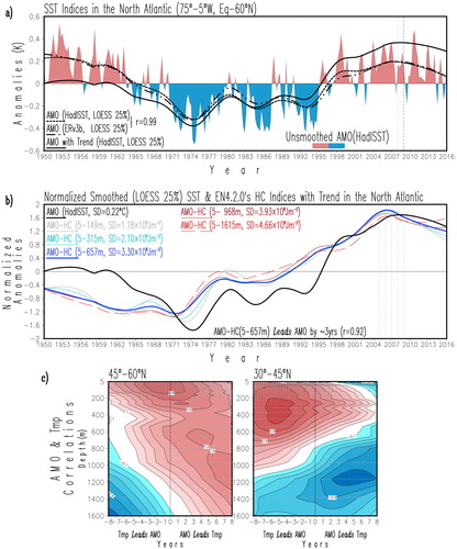
The evolution of undetrended AMO’s surface (SST) and subsurface (HC) thermal state is shown in Fig. 1b. The AMO-HC index is shown for various depths, and a comparison of the surface and subsurface thermal evolution suggests that during the period of a notable surface cooling (from 1960 to the mid-1970s), the subsurface North Atlantic was already shifting to a warming phase since 1970, however, both the surface and subsurface were in phase during this period preceding the most pronounced warming in the 1990s. There is a relative out-of-phase relationship between the surface and the subsurface North Atlantic in the second half of the twentieth century until 1998: surface/subsurface normalized anomalies were warmer/cooler than the subsurface/surface normalized anomalies in the period ∼1950–71, while conditions reversed in the period in ∼1971–98. The subsurface warming that occurred from the late-1980s to the mid-2000s is followed by cooling, which is observed to start early in the subsurface layers than at the surface with a lead time of ∼2–3 years. Further analysis of the temporal lead-lag between AMO (surface) and subsurface temperatures (Fig. 1c) indicates that near-surface temperature variations at depths of ∼50–200 m in the subpolar latitudes (45°N–60°N) take place almost simultaneously (∼0–1 years) with the AMO, while subsurface temperature variations at depths ∼300–500 m in the subtropical latitudes (30°N–45°N) appear to lead the surface ones from the AMO. This is consistent with the analysis done by Wang et al. (2010) indicating that temperature and salinity anomalies at subpolar latitudes lag those from subtropical latitudes by 8–9 years and this happens because oceanic advection. In essence, this picture suggests that the classical surface (basin-wide) definition of the AMO follows closely the near-surface variability at subpolar latitudes, but masks out the apparent leading influence of the variability of the subsurface layers in the subtropics.

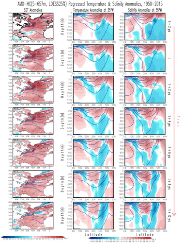
Low frequency variability at the subsurface in the North Atlantic, which seems to be leading surface variability, is captured by the HC-based AMO indices discussed above. A closer look at the structure associated with the Atlantic Multidecadal variability in the subsurface and its temporal evolution along the 35°W meridian is shown in Fig. 2 by regressing the new smoothed AMO-HC (5–657 m) index (dark blue line in Fig. 1b) on temperature and salinity detrended anomalies. The lead-lag figure shows upward propagation of cold/fresh subsurface anomalies from below 400 m in the 40°N–50°N band (perhaps along the climatological isotherms/isohalines), and deepening of the warm/saline near-surface (at ∼200 m depths and shallower) anomalies to ∼1200–1600 m in the 50°N–60°N band, which were present at the mature stage of the AMO-HC (t panel). Changes along the GS–NAC path are evident through the warm SST anomalies, and the temperature and salinity anomalies along the 40°N–50°N band from the depth-latitude profiles that, eventually, propagate along the NAC–SPG system; near-surface anomalies change sign 8 years after the mature phase of the AMO-HC (t + 8 yrs panel – also, Fig. 4.6 for HC (5–315 m) anomalies in Kavvada, 2014). Thus, it is reasonable to think that the cooling and warming trends at the surface and the subsurface are induced by ocean circulation (i.e. AMOC) and reflected by the Atlantic multidecadal variability (i.e. AMO). The structure of the trends and their subtropical to subpolar links will be explored in the next two subsections, but first the robustness of the basin-wide trends will be assessed.

Fig. 2. Lead/lag regressions on detrended SST, subsurface temperature and salinity of the normalized smoothed (LOESS25%) AMO-HC (5–657 m) index at 2-year intervals for the period 1950–2015. Left column shows the regressed SST anomalies (HadISST), while the central and right columns show the depth-latitude regressed temperature and salinity anomalies (EN4.2.0) along the 35°W meridian; temperature anomalies are in units of 10⁻¹ K and salinity are with no units. Time runs down as indicated by the long red arrow to the right. Red/blue shading corresponds to positive/negative anomalies. Solid black lines in the left column panels mark the climatological annual mean position of the subpolar and subtropical gyres using the −0.4 m and +0.4 m absolute dynamic topography values, respectively, and the dashed black line tracks the climatological annual-mean position of the North Atlantic current through the −0.1 m topographic contour from AVISO altimetry. Solid navy blue lines display the climatological, long-term means, in SST, subsurface temperatures and salinity; temperatures are displayed every 2 °C and salinity every 0.4 units. The grey stippling denotes significant grid points at the 95% confidence level based on a 2-tailed Student’s t-test.

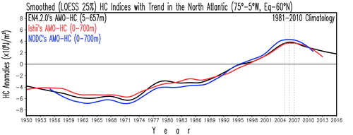
Trends in the AMO-HC index are similar when obtained from three different data sets as Fig. 3 shows, which displays the AMO-HC (0–700 m) indices all relative to the 1981–2010 climatology. As ocean observations are sparse and less reliable at greater depths, especially in the early record, the variations in heat content of the upper ocean (0–700 m) are further analyzed using several data sets (EN4.2.0, NODC and Ishii whose objective analyses differ in details as well in their choices of temporal resolution). All data sets are in agreement, especially in the representation of the impressive subsurface warming from the early-1970s to the mid-2000s, and the notable cooling thereafter.

Fig. 3. Area-averaged HC seasonal anomalies in the North Atlantic (75°W–5°W, Eq–60°N – AMO-HC indices) from different data sets: EN4.2.0 (black line) for the 5–567 m layer, and Ishii (red line), and NODC (navy-blue line) for the 0–700 m layer. Anomalies are calculated with respect to the common 1981–2010 climatology. Units are in 10⁸ J m⁻².

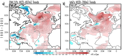
The AMO-HC indices readily identify the warming and cooling periods but do not provide any information on the regions within the North Atlantic basin where such trends are focused. The geographical distribution of the linear trend in upper HC for the period 1985–2005 (when the indices show a general warming) from the EN4.2.0 (5–657 m) and Ishii (0–700 m) data sets is shown in Fig. 4a, b. The largest warming trends from both data sets are in agreement, and they both highlight an almost general warming over the North Atlantic with the steepest trends in the SPG region. Also, consistent in both datasets is the presence of a cooling trend along the US east coast/GS path and regionally confined cooling trends to the east of the Flemish Cap at the western margin of the subtropical–subpolar gyre boundary. This latter region at the western margin of the subtropical and subpolar gyres is a dynamically complicated region (Marshall et al., 2001; Zhang, 2008; McCarthy et al., 2015; Buckley and Marshall, 2016). The latter paper referred to this as the transition zone, and argued to be a pacemaker for decadal AMOC variability.

Fig. 4. Linear trends of the upper-ocean HC in EN4.2.0 and Ishii data sets. Trends are displayed for the period 1985–2005 from (a) the 5–657 m layer from EN4.2.0, and (b) the 0–700 m layer from the Ishii data set. The period 1985–2005 corresponds to the warming period observed in the AMO and AMO-HC indices seen in Fig. 1. Red/blue shading corresponds to positive/negative trends. Units are in 10⁸ J m⁻²/year. Solid black lines mark the climatological annual mean position of the subpolar and subtropical gyres using the −0.4 m and +0.4 m absolute dynamic topography values, respectively, and the dashed black line tracks the climatological annual-mean position of the North Atlantic current through the −0.1 m topographic contour from AVISO altimetry. The grey stippling denotes significant grid points at the 95% confidence level based on a 2-tailed Student’s t-test.

3.2 Structure of decadal warming/cooling trends

Decadal trends in both upper HC and averaged salinity (5–657 m from EN4.2.0) show, before and after the subsurface maximum in 2006 (Fig. 5), distinctive features. The most pronounced warming and salinification is seen along the mean circulation during the warming period 1996–2005 (Häkkinen et al., 2013). During the cooling period 2006–2015, however, it is the central SPG that shows the largest cooling and freshening. It is also apparent that the trends along the GS path close to the North American coast are much warmer and more saline during the case of the cooling rather than during the warming period, and that the NAC is farther to the northeast in the case of the 2006–2015 cooling period, than in the case of the 1996–2005 warming period (see e.g. Häkkinen and Rhines, 2009; Häkkinen et al., 2011). The latter study finds that during warm periods, the wind-driven subtropical and subpolar gyres are weaker than normal, the subpolar density surfaces relax, which, in turn, lead to a westward shift of the subpolar front that permits warmer waters from the subtropics to invade the eastern SPNA (Hatun et al., 2005). Conversely, the cooling period, as observed in Fig. 5 (right column), is associated with an eastward shift of the subpolar front as shown recently by Zunino et al. (2017), their Fig. 8 (see also Bersch et al., 2007; note that this study only used data until 2004 and hence the implied eastward shift of the subpolar front during the recent cooling period is analogous to that of the early 1990s). In fact, variability in SST, upper-ocean HC and salt content extends further to the northeast for the cooling period than for the warming period (Supplementary Fig. 1S). The trend rates and spatial extent of the subsurface post-2006 North Atlantic cooling trend are larger than those of the pre-2006 warming trend. Note, however, that the warming trend in the 1996–2005 decade is part of a longer multidecadal warming trend as captured by the AMO-HC index and the 1985–2005 warming trend (Fig. 4). Similarly, the recent cooling trend is expected to last several more years (e.g. Yeager and Robson, 2017).

Fig. 5. Decadal linear trends in the upper-ocean HC and vertically averaged salinity for the 5–657 m layer before and after 2006 from EN4.2.0. Trends in HC are displayed in (a) for the period 1996–2005 and (b) for the period 2005–2015. Similarly, trends in salinity are displayed in (c) for the period 1996–2005 and d) for the period 2005–2015. The period 1996–2005 corresponds to the warming period observed in the AMO and AMO-HC indices, while the period 2005–2016 corresponds to the cooling period seen in Fig. 1. Red/blue shading corresponds to positive/negative trends in units of 10⁸ J m⁻²/year for HC and in units of 10⁻²/year in salinity. Solid black lines mark the climatological annual mean position of the subpolar and subtropical gyres using the −0.4 m and +0.4 m absolute dynamic topography values, respectively, and the dashed black line tracks the climatological annual mean position of the North Atlantic current through the −0.1 m topographic contour from AVISO altimetry. The grey stippling denotes significant grid points at the 95% confidence level based on a 2-tailed Student’s t-test.

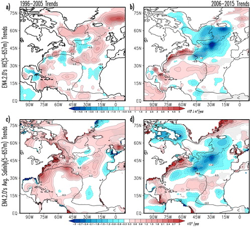
The structure of the cooling trend (Fig. 5) reflects the central role played by ocean dynamics rather than that caused by heat fluxes (Robson et al., 2016; Zhang et al., 2016; Delworth et al., 2017). The opposite-sign regions between the generalized cooling and freshening trends in the SPG region and warming and saline trends along the GS region are known to be a distinctive pattern of the AMOC, and the evolution of the reversed dipole pattern is thoroughly discussed in Zhang and Zhang (2015). The latter study shows that due to the existence of interior pathways, a warm anomaly propagating southward along the path of the deep western boundary current from the subpolar gyre will undergo different advection speeds (faster between 55°N and 34°N and slower south of there), which induces an anomalous heat convergence in the subpolar gyre (warming), but a heat divergence south of it (cooling). The time integral of this heat convergence/divergence is argued to give rise to this dipole. Note, however, that first the warming is enhanced in the SPG and then followed by a cooling in the GS region some years after. Zhang and Zhang (2015) also point out that the HC dipole between the SPG and GS regions is absent when there is no southward propagation of anomalies along the western boundary current.

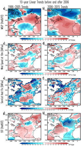
Analysis of trends at the atmosphere–ocean interface suggests that heat fluxes cannot be considered the only source of these trends as there is a mismatch between the structure of the trends in ocean–atmosphere heat fluxes and those in SSTs (Fig. 6). Trends in mean sea level pressure (MSLP) have an effect on the Icelandic low and Azores high or, in other words, on the mean northeasterly and westerly winds to the north and south of Iceland, respectively, as well as the mean easterly trade winds in the tropics. During the 1996–2005 warming trend years enhanced surface-wind trends along the coasts of Iceland, Greenland, Newfoundland, United States and in the central mid-Atlantic enclose weakened wind trends along the path of the NAC. This pattern drives negative surface flux trends around the rim of the SPG and positive surface flux trends in the centre of this gyre; the trends in surface fluxes should be producing a similar pattern of positive and negative SST trends if the latter were forced by the atmosphere. However, the structure of observed trends in SSTs shows a broad warming trend along the rim of the subpolar gyre and a confined cooling trend at its centre. During the 2006–2015 cooling period enhanced surface wind trends form a horse-shoe pattern appearing along the US and Newfoundland coasts that extends to Iceland and then southwestward along the Iberian Peninsula and western Africa until the tropics; the enhanced wind trends surround a region of weak wind trends in the centre of the basin from the subtropics to the midlatitudes around 45°N. The associated heat-flux trends follow this structure and suggest a cooling of the ocean over the Labrador basin, the SPG and the subtropical latitudes off the African coasts and a warming trend along the NAC and centre of the midlatitudes. However, trends in SSTs show a distinctive dipole pattern very much like the one seen in the HC trends suggesting that the atmosphere is not the main forcing of these ocean trends. Similar results are obtained if fields from NCEP/NCAR reanalysis (Kalnay et al., 1996) are used. In fact, these results chime with those by Robson et al. (2016 – Fig. 2) regarding the oceanic nature of the observed warming and cooling trends before and after 2005.

Fig. 6. Decadal trends at the atmosphere–ocean interphase before and after 2006. Panels in the left column show trends for the period 1996–2005, those in the right column for the period 2006–2010. Trends in mean sea level pressure are in panels (a) and (b) in units of 10⁻² h Pa/year from HadSLP2; trends in wind speed at 10 m are in panels (c) and (d) in units of 10⁻² m s⁻¹/year from OAFlux; trends in sensible plus latent heat flux are in panels (e) and (f) in units of Wm⁻²/year from OAFlux where positive trends indicate warming of the ocean; trends in SST are in panels (g) and (h) in units of 10⁻² K/year from HadISST. Red/blue shading corresponds to positive/negative trends. Solid black lines mark the climatological annual-mean position of the subpolar and subtropical gyres using the −0.4 m and +0.4 m absolute dynamic topography values, respectively, and the dashed black line tracks the climatological annual mean position of the North Atlantic current through the −0.1 m topographic contour from AVISO altimetry. Similar results are obtained by using NCEP/NCAR reanalysis data. The grey stippling denotes significant grid points at the 95% confidence level based on a 2-tailed Student’s t-test.

While it is important to analyze the structure of the decadal trends, it is also illustrative to analyze the mean decadal anomalies and the evolution of both decadal anomalies and trends in order to elucidate an underlying mechanism. The structure of the warming and decadal trends before and after 2006 shows some features over the SPG and the GS–NAC system that resemble the evolution of upper-ocean HC associated with the AMO discussed in Kavvada et al. (2013), where contrasting HC anomalies between the GS–NAC and SPG regions, associated with the AMO, change signs within a decade. Hence, it should be taken into consideration that decadal variations in the GS–NAC–SPG system may induce decadal trends. The basin-wide AMO and AMO-HC time series in Fig. 1 show decadal cooling trends only in two periods: the current one after 2006, already described, and an early one in the 1960s; the cooling trend in the 1960s is more pronounced at the surface (AMO) than in the subsurface layers (AMO-HC) and ceases later in the mid-70s.

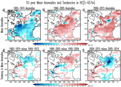
Figure 7 contrasts 10-yr mean anomalies and their tendencies from one decade to the next one after one year in the upper HC for the 1965–1974, 1996–2005 and the 2006–2015 decades in order to highlight the regions changing the most from one decade to the immediate one in the smoothed (decadal) data. Independent of the sign (or the decade), the mean anomalies of one sign occupy almost the entire basin with maximum values along the GS region and have anomalies of the opposite sign in the SPNA region with varied extents (Fig. 7, upper row). It is significant to note the following two things. Firstly, these anomalies in the SPNA region occupy different areas within the region but all show anomalies just to the east of the Flemish Cap around 45°W, 45°N, that is, a region where the GS current in its northeastward path meets the southward side of the SPG. Secondly, the similarities between the mean anomalies for the 1996–2005 warming period and those for the 2006–2015 cooling period are notable. The 2006–2015 anomalies of one sign over the Reykjanes Ridge and anomalies of the opposite sign in the Iceland basin appear to have developed from the anomalies in the 1996–2005 decade: the cold central-gyre anomaly and the anomaly to the east of the Flemish cap. It has been argued by Nigam et al. (2018) that such structures in HC may be the result of a southward intrusion of subpolar waters through the Newfoundland Basin, which promotes a detachment of GS anomalies in its northeastern section that eventually cross and invade the subpolar region via the NAC pathways. Along this line, it is seen that the tendency in the decadal pattern (Fig. 7, lower row) highlights the regions of largest change from the previous decade and include the GS–NAC–SPG regions, which are the same regions where the largest trends are found (Fig. 5, upper row for trends before and after 2006). Mean anomalies in vertically averaged salinity and their tendencies (Supplementary Fig. 2S) highlight that anomalously cold and warm anomalies are accompanied by fresh and saline anomalies, respectively, which reinforces the role for ocean circulation as the main driver of these large-scale heat anomalies.

Fig. 7. Decadal mean anomalies and their change in upper HC (5–657 m) during three different decades from EN4.2.0. Panels in the left column are for the 1965–1974 decade, panels in the central column for the 1996–2005 decade, and panels in the right column are for the 2006–2015 decade. Mean anomalies are in panels (a), (b) and (c) in units of 10⁸ J m⁻². Tendencies in mean 10-year anomalies between two consecutive periods are in (d) 1965–1974 and 1964–1973, (e) 1996–2005 and 1995–2004 and (f) 2006–2015 and 2005–2014 in units of 10⁸ J m⁻². Red/blue shading corresponds to positive/negative anomalies and their change. Solid black lines mark the climatological annual mean position of the subpolar and subtropical gyres using the −0.4 m and +0.4 m absolute dynamic topography values, respectively, and the dashed black line tracks the climatological annual-mean position of the North Atlantic current through the −0.1 m topographic contour from AVISO altimetry.

3.3 Variability in the subpolar North Atlantic and the Gulf stream

The previous two sections have shown the prominence that the subpolar (via the SPG and associated currents) and subtropical (via the GS) regions have in shaping the observed decadal anomalies and, in consequence, the decadal trends. Because near-surface temperatures in the subpolar latitudes occur (almost) simultaneously with the AMO (Fig. 1b), attention is focused on this region. A series of indices are created for area-averaged SST and heat-content anomalies within the SPG region (60°W–10°W, 45°N–65°N). These indices are highly coherent and show maximum amplitude in 2006–2007 before shifting to a cooling trend (Fig. 8a), which is steeper in the subpolar region than in the whole basin, suggesting the SPG plays a prominent role in leading the basin-wide trends. The SPG surface thermal variations lag those from the subsurface subtropics by ∼5 years (Fig. 8b, right panel), and propagate with time to the subsurface layers and reach the 1000 m column around 5 years later (Fig. 8b, left panel). In particular, the upper ocean layer of the SPNA region was under cold and fresh conditions during the period 1970–1995, and has been under anomalous warm and saline conditions since 1995, reaching maximum anomalies and penetration around 2006 (Fig. 9). A reversal to cold and fresh conditions start to appear in the region in 2015, suggesting a return to a cold phase seen in the 90s, if not more pronounced this time (see e.g. Yashayaev and Loder, 2016). It is thus important to note that decadal cooling was already underway since mid-2000s (Zunino et al., 2017, their Fig. 9), which makes the so called ‘cold blob’ (Duchez et al., 2016; Josey et al., 2018) only part of decade-long cooling trend that intensified during winter 2014 due to extreme surface heat loss (Zunino et al., 2017; Josey et al., 2018).

Fig. 8. Subpolar North Atlantic (SPNA) indices for the period 1950–2015. Indices are created by area-averaging anomalies over the subpolar domain (60°W–10°W, 45°N–60°N). (a) Normalized undetrended subpolar indices from HadISST’s SST anomalies (black heavy line), and EN4.2.0 HC anomalies for the layers 5–149 m (gray line), 5–315 m (thin light blue line), 5–657 m (thick blue line), 5–968 m (thin dark-red line) and 5–1615 m layer (thin long-dash red line). Normalization is done by dividing the smoothed index by its standard deviation in units of K for the SST index and 10⁸ J m⁻² for the heat content indices as shown in the inset. Maximum correlations between the surface and subsurface indices are displayed at the bottom right indicating that surface anomalies lead those at the subsurface over the subpolar region. Note that the indices in this region show cooling trends after 2006 which are larger than the all-basin indices in Fig. 1b. (b) Profiles of lead/lag correlations between smoothed detrended surface SPNA index and smoothed detrended subsurface temperature anomalies at the 45°N–60°N and 30°N–45°N latitude bands; the vertical axis is depth in m, horizontal axis is lead/lag in years, and red/blue shading corresponds to positive/negative correlations; the grey stippling denotes significant grid points at the 95% confidence level based on a 2-tailed Student’s t-test.

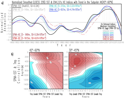
Fig. 9. Area-averaged wind anomalies and profiles of subsurface water property anomalies in the subpolar region (60°W–10°W, 45°N–60°N) from 1950 to 2015. (a) Wind-speed anomalies at 850 mb from the NCEP/NCAR reanalysis, (b) temperature (shaded) and salinity (contours) anomalies, (c) density (shaded) and salinity forced density anomalies (contours) and (d) density (shaded) and temperature forced density anomalies (contours). Salinity/temperature-forced density anomalies are calculated considering climatological temperature/salinity in the UNESCO formula. Wind speed is in ms⁻¹, temperature in K, salinity with no units, and densities are in kgm⁻³. Red/blue shading and continuous/dash lines correspond to positive/negative anomalies.

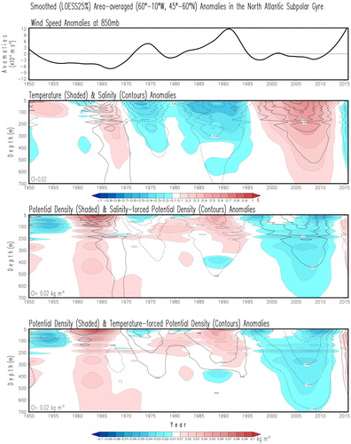
It is apparent that temperature and salinity anomalies deepen with time, and that the cold and warm upper-ocean anomalies co-vary with positive and negative wind speed anomalies, respectively, however the warming in the 2000s is not commensurable to the weak reduction in wind speed. It is important to point out that changes in HC can result from changes in air–sea heat fluxes and the convergence/divergence of ocean heat transports (see e.g. Barrier et al., 2014), with the latter a result of not just AMOC-related changes, but also wind-driven. An important aspect to note in Fig. 9 is that the potential density anomalies in the subpolar region are largely responsive to the temperature anomalies, except around 1972 when the salinity effect (Great salinity anomaly effects, Dickson et al., 1988) on density dominated over the temperature effect.

Anomalous conditions over the SPNA region (as over the entire basin) seem to be preceded by anomalous conditions at the subsurface in the subtropics (Fig. 8b, right panel). On the other hand, variability on this subtropical region is largely confined to the western basin along the domain of the GS current (Supplementary Fig. 1S), so it is reasonable to expect that an index for the northward excursions of the GS current (Fig. 10a) leads the subsurface variability of the SPNA region as a whole (by ∼13 years); but even more revelatory is the fact that the lead increases from the northeast Atlantic at ∼9 years, and to the central and western SPNA at 13 and 14 years, respectively (Fig. 10b, c). Similar lag years with the GS index are obtained if instead of using the area-averaged HC over the three different basins (Iceland Basin, Irminger Sea and Labrador Sea) along the mean circulation, specific points within them are used. In fact, regressions of the smoothed GS index on SST, upper HC and averaged salinity show how in a span of about 12 years warm and saline anomalies from the GS reach the subpolar region (Fig. 11). The propagating signal along the GS–NAC–SPNA path with an 8–14-year time scale agree with the findings of Sutton and Allen (1997) of northward advection of SST anomalies in North Atlantic, with the modelling findings of Teng et al. (2011) of advection of subsurface temperatures, and recently supported by Årthun et al. (2017). The latter investigators demonstrated that poleward propagating SST anomalies from the northern extension of the Gulf Stream all the way to Nordic Seas are independent of the prevailing atmospheric circulation and predominantly controlled by ocean dynamics. Note, however, that the spatial progression of anomalies in Fig. 11 appear to be better captured by upper-ocean HC rather than by SSTs, which is likely due to the subsurface nature of the GS index (Joyce and Zhang, 2010).

Fig. 10. The Gulf Stream index and its relationship to the upper-ocean HC (5–657 m)-based subpolar North Atlantic (SPNA) indices for the period 1954–2012. (a) Normalized unsmoothed GS index (shaded), smoothed (LOESS25%) GS index and undetrended smoothed (LOESS25%) SPNA HC index for the layers 5–657 m (blue line). (b) Map showing the regions where the GS and SPNA indices are defined. The GS index was obtained from temperature data at 200 m within the domain in the black rectangle (75°W–50°W, 33°N–43°N); the SPNA index used in (a) is area-averaged over the blue rectangle (60°W–10°W, 45°N–60°N); a western SPNA index is defined by area-averaging over the red rectangle (60°W–44°W, 45°N–60°N); a central SPNA index is defined by area-averaging over the green rectangle (44°W–27°W, 45°N–60°N); an eastern SPNA index is defined by area-averaging over the light blue rectangle (27°W–10°W, 45°N–60°N). (c) Lead/lag correlations between smoothed detrended GS index and SPNA HC-based indices. Note that the GS leads the subpolar indices and that the farther to the west the SPNA index is defined, the larger is the lag.

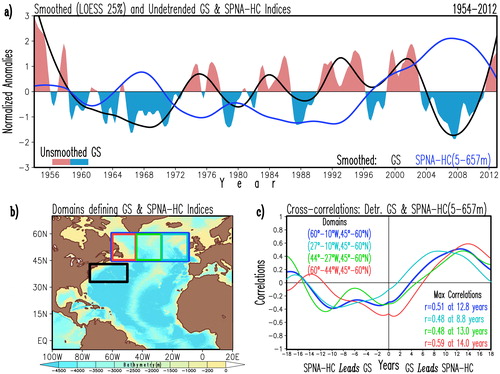
Fig. 11. Lead-lag regressions on detrended anomalies of the normalized smoothed (LOESS25%) GS index for the period 1954–2012. Panels in the left column show regressed SST anomalies in units of 10⁻¹ K, those in the central column display upper-ocean HC (5–657 m) anomalies in units of 10⁸ J m⁻², and panels in the right column show vertically averaged (5–657 m) salinity anomalies with no units at 2-year intervals from t − 6 years (top row) to simultaneous (central row) to t + 6 years (bottom row). Time runs down as indicated by the long red arrow to the left. Red/blue shading represents positive/negative anomalies. Solid black lines mark the climatological annual mean position of the subpolar and subtropical gyres using the −0.4 m and +0.4 m absolute dynamic topography values, respectively, and the dashed black line tracks the climatological annual-mean position of the North Atlantic current through the −0.1m topographic contour from AVISO altimetry. The grey stippling denotes significant grid points at the 95% confidence level based on a 2-tailed Student’s t-test.

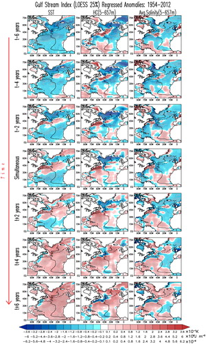
Figure 11 further shows that while the GS is advecting anomalies in a northeasterly direction, anomalies of opposite sign are being displaced westwards by the northern branch of the SPG to eventually turn south in front of the Newfoundland coast; the southward displacement of anomalies stops around the Flemish Cap (45°W, 45°N) where it cuts off the GS current and leaves clipped anomalies to continue their northeastwards displacement toward the Icelandic and Irminger basins (Nigam et al., 2018). Similarities between regressed SST anomalies from the GS index at t − 4 years (Fig. 11, panel t + 4 yrs) and those from the AMO-HC (5–657 m), assuming its negative phase, at t + 10 years (Fig. 2, panel t + 10 yrs) are worth noting, suggesting a link between these phenomena. However, the mechanisms through which the GS and the AMO are connected is not a goal in the current paper, and the reader is referred to the recent study by Nigam et al. (2018).

4. Discussion and conclusions

The subsurface spatiotemporal structure of the North Atlantic Ocean is analyzed in the context of the recent cooling trend. In this analysis a vertically integrated (5–657 m) ocean heat content AMO index has been proposed in an effort to capture the thermal state of the ocean and not just that of the sea surface as in the canonical AMO SST-based indices, where both are defined over the same region. Regressions of the traditional AMO SST index and our new AMO-HC (5–657 m) index on subsurface temperatures and salinity anomalies highlights decadal interactions not only between the tropical, subtropical and subpolar latitudes but also between subsurface and surface anomalies with the potential to provoke decadal trends in the North Atlantic Ocean. The use of this HC-based index has been revealing as it indicates that: (1) The North Atlantic subsurface had a warming trend since the mid-1980s to the mid-2000s, a feature that was also present at the surface with an evident lag of ∼3 years with respect to the AMO-HC (5–657 m) index. (2) The North Atlantic subsurface shows a cooling trend since the mid-2000s, a feature that is leading the ocean surface and one with significant implications for predicting future North Atlantic climate (Yeager and Robson, 2017). (3) The traditional surface AMO index (SST-based) lags the subsurface indices (HC-based) with the leading time being latitude dependent: deeper waters centred around 350 m in the subtropics (30°N–45°N) lead by ∼5 years, while the surface waters centred around 50–100 m depths in the midlatitudes (45°N–60°N) lead by ∼0–1 year.

The spatial structure of the trends in the North Atlantic after 2006 suggests a link with decadal AMOC variability (Jackson et al., 2016; Robson et al., 2016), but other processes related to gyre-circulation changes could also have played a role (Bersch et al., 2007; Häkkinen et al., 2011; Piecuch et al., 2017). In particular, Piecuch et al. (2017) suggest a role for mid-latitude wind stress curl changes at the subpolar-subtropical gyre boundary for the development of the recent decadal cooling of the SPNA. However, Robson et al. (2016) argue for changes of the Labrador Sea density and hence the overturning. Jackson et al. (2016) showed using an ocean reanalysis that the AMOC started a decadal decline around mid-2000s and therefore part of an internal, not forced, variability since it is a recovery from the earlier strengthening. It, thus, appears that both the gyre and overturning circulation likely had an effect on the observed decadal climate reversal to a cooling trend (Robson et al., 2016; Piecuch et al., 2017).

The structure of the 20-year warming trend before 2006 is similar to the 10-year warming trend before 2006, albeit weaker (cf. Figs. 4 and 5). In both cases warming trends surround cold trends along the GS–NAC meeting point with the cold trends reaching higher northern latitudes in the recent 10-year period than in the 20-year period before 2006. The incipient cooling trend along the GS–NAC system before 2006 evolves to the cooling trend covering the NAC–SPG region in the following 10 years after 2006. Analysis of surface heat fluxes only partially explains the observed SST warming and cooling trends before and after 2006, suggesting that ocean dynamical processes are the primary source and hence critical to the observed trends (Robson et al., 2016; Zhang et al., 2016; Piecuch et al., 2017; Zhang, 2017).

Mean decadal anomalies, their change and trends all suggest a link with variability generated by the GS–NAC–SPG system. It is not simple to locate where conditions start but at some point in the evolution of the mean HC and salinity decadal anomalies these are of one sign along the GS region, and of opposite sign in the eastern portion of the SPG region. While the anomalies along the GS move northeastwards, anomalies from the SPG move southwards along the North American coasts and the western boundary. The southward displacement of anomalies eventually reaches the region where the anomalies of opposite sign are driven by the GS current and ‘clip them off’ to follow the NAC. This southward extent of anomalies of one sign and the cutoff anomalies of the opposite sign sets up conditions to reverse the sign of the anomalies in both the GS and SPNA regions; an interaction that adds to the list of complex processes that are at the core of the North Atlantic decadal variability (Zhang, 2008; Joyce and Zhang, 2010; Zhang and Zhang, 2015; Delworth et al., 2017; Nigam et al., 2018).

Trends, variability as well as the near-surface subpolar and subsurface subtropical connection captured by the basin-wide (AMO and AMO-HC) indices are also identified by SPNA (SST- and HC-based) indices. The warming and cooling trends distinguished from the whole-basin indices (AMO and AMO-HC) are also found in the SPNA indices (SST- and HC-based) but with steeper values. Surface anomalies in the SPNA region as a whole penetrates into the deeper layers with time, however, water properties (i.e. density) are not homogeneous as the eastern and western SPG is more sensitive to changes in temperature and salinity, respectively.

On the other hand, and as in the case of the whole basin characterized with the AMO index, surface variability in the SPNA region is led by variability in the subsurface subtropics (30°N–45°N), and the main source of variability in the Atlantic Ocean in this latitudinal band comes from the Gulf Stream itself. The GS in fact leads variability in the upper HC (5–657 m) over the SPNA region as a whole by ∼13 years, but the lead increases from east to west from ∼9 years (over the Iceland Basin) to ∼13 years (over the Irminger Sea) to ∼14 years (over the Labrador Sea). This connection is reflected in regressions of a GS index on SST, upper-ocean HC and salt content that present coherent anomalies of one sign along the GS region and anomalies of the opposite sign over the SPNA region that evolve and change sign along the GS–NAC–SPG system on decadal time scales.

A better understanding of the decadal variations in the Atlantic is of paramount importance for the societies inhabiting the continents around it. Warming of the North Atlantic waters has been linked to multiyear droughts over the central United States (e.g. Nigam et al., 2011), anomalous rainfall over western Europe and the Sahel (e.g. Sutton and Hodson, 2005; Nigam and Ruiz-Barradas, 2016) and increased hurricane activity (e.g. Goldenberg et al., 2001; Nigam and Guan, 2011) while the opposite regional climate conditions, including heat waves over Europe (Duchez et al., 2016; Josey et al. 2018), are observed during colder episodes of the North Atlantic waters.

Supplemental data

Supplemental data for this article can be accessed here: http://10.0.4.56/16000870.2018.1481688.

Acknowledgements

The authors are grateful to T. Joyce for making the Gulf Stream index available. Argyro Kavvada performed preliminary analysis of the HC-based AMO indices as part of her doctoral thesis at the University of Maryland in 2014.

Disclosure statement

No potential conflict of interest was reported by the authors.

Additional information

Funding

LC acknowledges funding through the iNcREASE project. AR-B and SN gratefully acknowledge support from the US National Science Foundation through the grant AGS1439940.

References

- Allan, R. J. and Ansell, T. J. 2006. A new globally complete monthly historical mean sea level pressure data set (HadSLP2): 1850–2004. J. Clim. 19, 5816–5842. DOI:10.1175/JCLI3937.1.
- Årthun, M., Eldevik, T., Viste, E., Drange, H., Furevik, T. and co-authors. 2017. Skillful prediction of northern climate provided by the ocean. Nat. Comms. 8, 15875. DOI:10.1038/ncomms15875.
- Barrier, N., Cassou, C., Deshayes, J. and Treguier, A.-M. 2014. Response of North Atlantic Ocean circulation to atmospheric weather regimes. J. Phys. Oceanogr. 44, 179–201. DOI:10.1175/JPO-D-12-0217.1.
- Bersch, M., Yashayaev, I. and Koltermann, K. P. 2007. Recent changes of the thermohaline circulation in the subpolar North Atlantic. Ocean Dyn. 57, 223–235. DOI:10.1007/s10236-007-0104-7.
- Bjerknes, J. 1964. Atlantic Air–Sea Interaction. Advances in Geophysics, Vol. 10. Academic Press, New York, 1964, pp. 1–82.
- Boyer, T. P., Levitus, S., Antonov, J., Locarnini, R. and Garcia, H. 2005. Linear trends in salinity for the World Ocean, 1955–1998. Geophys. Res. Lett. 32, L01604. DOI:10.1029/2004GL021791.
- Bryan, K. and Stouffer, R. 1991. A note on Bjerknes’ hypothesis for North Atlantic variability. J. Marine Syst. 1, 229–241. DOI:10.1016/0924-7963(91)90029-T.
- Buckley, M. W. and Marshall, J. 2016. Observations, inferences, and mechanisms of Atlantic meridional overturning circulation variability: a review. Rev. Geophys. 54, 5. DOI:10.1002/2015RG000493.
- Cheng, L., Trenberth, K. E., Fasullo, J., Boyer, T., Abraham, J. and co-authors. 2017. Improved estimates of ocean heat content from 1960 to 2015. Sci. Adv. 3, e1601545. DOI:10.1126/sciadv.1601545.
- Cleveland, W. S. and Loader, C. L. 1996. Smoothing by local regression: principles and methods. In: Statistical Theory and Computational Aspects of Smoothing (eds. W. Haerdle and M. G. Schimek), Springer, New York, pp. 10–49.
- Delworth, T. L., Zeng, F., Zhang, L., Zhang, R., Vecchi, G. A. and co-authors. 2017. The central role of ocean dynamics in connecting the North Atlantic Oscillation to the extratropical component of the Atlantic Multidecadal Oscillation. J. Climate 30, 3789. DOI:10.1175/JCLI-D-16-0358.1.
- Deser, C., Alexander, M. A., Xie, S.-P. and Phillips, A. 2010. Sea surface temperature variability: patterns and mechanisms. Annu. Rev. Mar. Sci. 2, 115–143. DOI:10.1146/annurev-marine-120408-151453.
- Dickson, R. R., Meincke, J., Malmberg, S.-A. and Lee, A. J. 1988. The “great salinity anomaly” in the Northern North Atlantic 1968–1982. Prog. Oceanog. 20, 103–151. DOI:10.1016/0079-6611(88)90049-3.
- Drews, A. and Greatbatch, R. 2016. Atlantic multidecadal varability in a model with an improved North Atlantic current. Geophys. Res. Lett. 43, 8199–8206.
- Duchez, A., Frajka-Williams, E., Josey, S. A., Evans, D. G., Grist, J. P., and co-authors. 2016. Drivers of exceptionally cold North Atlantic Ocean temperatures and their link to the 2015 European heat wave. Environ. Res. Lett. 11. DOI: 10.1088/1748-9326/11/7/074004.
- Enfield, D. B., Mestas-Nuñez, A. M. and Trimble, P. J. 2001. The Atlantic Multidecadal Oscillation and its relationship to rainfall and river flows in the continental US. Geophys. Res. Lett. 28, 2077–2080. DOI:10.1029/2000GL012745.
- Frankignoul, C. and Hasselmann, K. 1977. Stochastic climate models. Part 2. Application to sea-surface temperature variability and thermocline variability. Tellus 29, 289–305.
- Gill, A. E. 1982. Atmosphere–Ocean Dynamics. International Geophysics Series, Vol. 30. Academic Press, London, pp. 599–600.
- Good, S. A., Martin, M. J. and Rayner, N. A. 2013. EN4: quality controlled ocean temperature and salinity profiles and monthly objective analyses with uncertainty estimates. J. Geophys. Res. Oceans 118, 6704–6716. DOI:10.1002/2013JC009067.
- Goldenberg, S. B., Landsea, C. W., Mestas-Nuñez, A. M. and Gray, W. M. 2001. The recent increase in Atlantic hurricane activity: causes and implications. Science 293, 474–479. DOI:10.1126/science.1060040.
- Gouretski, V. and Reseghetti, F. 2010. On depth and temperature biases in bathythermograph data: development of a new correction scheme based on analysis of a global ocean database. Deep Sea Res., Part I 57, 812–833. DOI:10.1016/j.dsr.2010.03.011.
- Guan, B. and Nigam, S. 2009. Analysis of Atlantic SST variability factoring inter-basin links and the secular trend: clarified structure of the Atlantic Multidecadal Oscillation. J. Climate 22, 4228–4240. DOI:10.1175/2009JCLI2921.1.
- Häkkinen, S. 2001. Variability in sea surface height: a qualitative measure for the meridional overturning in the North Atlantic. J. Geophys. Res. 106, 13837–13848.
- Häkkinen, S. and Rhines, P. B. 2009. Shifting surface currents in the northern North Atlantic Ocean. J. Geophys. Res. 114, C04005. DOI:10.1029/2008JC004883.
- Häkkinen, S., Rhines, P. B. and Worthen, D. L. 2011. Warm and saline events embedded in the meridional circulation of the northern North Atlantic. J. Geophys. Res. 116, C03006. DOI:10.1029/2010JC006275.
- Häkkinen, S., Rhines, P. B. and Worthen, D. L. 2013. Northern North Atlantic sea surface heightand ocean heat content variability. J. Geophys. Res. Oceans 118, 3670–3678. DOI:10.1002/jgrc.20268.
- Häkkinen, S., Rhines, P. B. and Worthen, D. L. 2015. Heat content variability in the North Atlantic Ocean in ocean reanalyses. Geophys. Res. Lett 42, 2901–42909. DOI:10.1002/2015GL063299.
- Häkkinen, S., Rhines, P. B. and Worthen, D. L. 2016. Warming of the global ocean: spatial structure and water-mass trends. J. Climate 29, 4949–4963. DOI:10.1175/JCLI-D-15-0607.1.
- Hatun, H., Sandø, A.-B., Drange, H., Hansen, B. and Valdimarsson, H. 2005. Influence of the Atlantic subpolar gyre on the thermohaline circulation. Science 309, 1841–1844. DOI:10.1126/science.1114777.
- Ishii, M. and Kimoto, M. 2009. Reevaluation of historical ocean heat content variations with time-varying XBT and MBT depth bias corrections. J. Oceanogr. 65, 287–299. DOI:10.1007/s10872-009-0027-7.
- Jackson, L. C., Peterson, K. A., Roberts, C. D. and Wood, R. A. 2016. Recent slowing of Atlantic overturning circulation as a recovery from earlier strengthening. Nature Geosci. 9, 518–522. DOI:10.1038/ngeo2715.
- Josey, S. A., Hirschi, J. J.-M., Sinha, B., Duchez, A., Grist, J. P. and Marsh, R. 2018. The recent Atlantic cold anomaly: causes, consequences, and related phenomena. Ann. Rev. Mar. Sci. 10, 475–501. DOI:10.1146/annurev-marine-121916-063102.
- Joyce, T. M., Deser, C. and Spall, M. A. 2000. The relation between decadal variability of subtropical mode water and the North Atlantic oscillation. J. Climate 13, 2550–2569. DOI:10.1175/1520-0442(2000)013<2550:TRBDVO>2.0.CO;2.
- Joyce, T. M. and Zhang, R. 2010. On the path of the Gulf stream and the Atlantic meridional circulation. J. Climate 23, 3146–3154. DOI:10.1175/2010JCLI3310.1.
- Kalnay, E., Kanamitsu, M., Kistler, R., Collins, W., Deaven, D. and co-authors. 1996. The NCEP/NCAR 40-year reanalysis project. Bull. Amer. Meteor. Soc. 77, 437–471. DOI:10.1175/1520-0477(1996)077<0437:TNYRP>2.0.CO;2.
- Kavvada, A., Ruiz-Barradas, A. and Nigam, S. 2013. AMO’s structure and climate footprint in observations and IPCC AR5 climate simulations. Clim. Dyn. 41, 1345–1364. DOI:10.1007/s00382-013-1712-1.
- Kavvada A. 2014. Atlantic multidecadal variability: Surface and subsurface thermohaline structure and hydroclimate impacts. Ph. D. thesis. University of Maryland. 153 pp.
- Marshall, J., Johnson, H. and Goodman, J. 2001. A study of the interaction of the north Atlantic oscillation with ocean circulation. J. Climate 14, 1399–1421. DOI:10.1175/1520-0442(2001)014<1399:ASOTIO>2.0.CO;2.
- McCarthy, G. D., Haigh, I. D., Hirschi, J. J.-M., Grist, J. P. and Smeed, D. A. 2015. Ocean impact on decadal Atlantic climate variability revealed by sea-level observations. Nature 521, 508–510. DOI:10.1038/nature14491.
- Metz, W. 1991. Optimal relationship of large-scale flow patterns and the Barotropic feedback due to high-frequency Eddies. J. Atmos. Sci. 48, 1141–1159. DOI:10.1175/1520-0469(1991)048<1141:OROLSF>2.0.CO;2.
- Nigam, S. and Guan, B. 2011. Atlantic tropical cyclones in the 20th century: natural variability and secular change in cyclone count. Clim. Dyn. 36, 2279–2293. DOI:10.1007/s00382-010-0908-x.
- Nigam, S., Guan, B. and Ruiz-Barradas, A. 2011. Key role of the Atlantic multidecadal oscillation in 20th century drought and wet periods over the Great Plains. Geophys. Res. Lett. 38. DOI:10.1029/2011GL048650.
- Nigam, S. and Ruiz-Barradas, A. 2016. Key Role of the Atlantic Multidecadal Oscillation in 20th Century Drought and Wet Periods over the US Great Plains and the Sahel. Chapter 21 In: The Book: Dynamics and Predictability of Large-scale High-Impact Weather and Climate Events (eds. Jianping Li, Richard Swinbank, Hans Volkert and Richard Grotjahn), Cambridge University Press, Cambridge.
- Nigam, S., Ruiz-Barradas, A. and Chafik, L. 2018. Gulf stream excursions and sectional detachments generate the decadal pulses in the Atlantic multidecadal dscillation. J. Climate 31, 2853–2870.
- Piecuch, C. G., Ponte, R. M., Little, C. M., Buckley, M. W. and Fukumori, I. 2017. Mechanisms underlying recent decadal changes in subpolar North Atlantic Ocean heat content. J. Geophys. Res. Oceans 122, 7181–7197. DOI:10.1002/2017JC012845.
- Pujol, M.-I., Faugère, Y., Taburet, G., Dupuy, S., Pelloquin, C. and co-authors. 2016. DUACS DT2014: the new multi-mission altimeter data set reprocessed over 20 years. Ocean Sci. 12, 1067–1090. DOI:10.5194/os-12-1067-2016.
- Rahmstorf, S., Box, J. E., Feulner, G., Mann, M. E., Robinson, A. and co-authors. 2015. Exceptional twentieth-century slowdown in the Atlantic Ocean overturning circulation. Nat. Clim. Change 5, 475. DOI:10.1038/nclimate2554.
- Rayner, N. A., Parker, D. E., Horton, E. B., Folland, C. K., Alexander, L. V. and co-authors. 2003. Global analyses of sea surface temperature, sea ice, and night marine air temperature since the late nineteenth century. J. Geophys. Res. 108, 4407. DOI:10.1029/2002JD002670.
- Reverdin, G., Niiler, P. P. and Valdimarsson, H. 2003. North Atlantic surface currents. J. Geophys. Res. 108, 3002. DOI:10.1029/2001JC001020.
- Reverdin, G. 2010. North Atlantic subpolar gyre surface variability (1895–2009). J. Climate 23, 4571–4584. DOI:10.1175/2010JCLI3493.1.
- Robson, J., Sutton, R. and Smith, D. 2014. Decadal predictions of the cooling and freshening of the North Atlantic in the 1960s and the role of ocean circulation. Clim. Dyn. 42, 2353–2365. DOI:10.1007/s00382-014-2115-7.
- Robson, J., Ortega, P. and Sutton, R. 2016. A reversal of climate trends in the North Atlantic since 2005. Nature Geosci. 9, 513. DOI:10.1038/ngeo2727.
- Santer, B. D., Wigley, T. L. M., Boyle, J. S., Gaffen, D. J., Hnilo, J. J. and co-authors. 2000. Statistical significance of trends and trend differences in layer-average atmospheric temperature time series. J. Geophys. Res. 105, 7337–7356.
- Smith, T. M., Reynolds, R. W., Peterson, T. C. and Lawrimore, J. 2008. Improvements to NOAA’s historical merged land–ocean surface temperature analysis (1880–2006). J. Climate 21, 2283–2296. DOI:10.1175/2007JCLI2100.1.
- Sutton, R. T. and Allen, M. R. 1997. Decadal predictability of North Atlantic sea surface temperature and climate. Nature 388, 563–567. DOI:10.1038/41523.
- Sutton, R. T. and Hodson, D. L. R. 2005. Atlantic Ocean forcing of North American and European summer climate. Science 309, 115–118. DOI:10.1126/science.1109496.
- Teng, H., Branstator, G. and Meehl, G. A. 2011. Predictability of the Atlantic overturning circulation and associated surface patterns in two CCSM3 climate change ensemble experiments. J. Climate 24, 6054–6076. DOI:10.1175/2011JCLI4207.1.
- Wang, C., Xie, S.-P. and Carton, J. A. 2004. A global survey of ocean–atmosphere interaction and climate variability, in Earth's Climate: the ocean–atmosphere interaction. AGU Geophys. Monogr. Series 147, 1–19.
- Wang, C., Dong, S. and Munoz, E. 2010. Seawater density variations in the North Atlantic and the Atlantic meridional overturning circulation. Clim. Dyn. 34, 953–968. DOI:10.1007/s00382-009-0560-5.
- Wang, C. and Zhang, L. 2013. Multidecadal ocean temperature and salinity variability in the tropical North Atlantic: linking with the AMO, AMOC, and subtropical cell. J. Climate 26, 6137–6162. DOI:10.1175/JCLI-D-12-00721.1.
- Yashayaev, I. and Loder, J. W. 2016. Recurrent replenishment of Labrador Sea Water and associated decadal scale variability. J. Geophys. Res. Oceans 121, 8095–8114. DOI:10.1002/2016JC012046.
- Yeager, S. G. and Robson, J. I. 2017. Recent progress in understanding and predicting Atlantic decadal climate variability. Curr. Clim. Change Rep. 3, 112–127. DOI:10.1007/s40641-017-0064-z.
- Yu, L., Jin, X. and Weller, R. A. 2008. Multidecade Global Flux Datasets from the Objectively Analyzed Air-sea Fluxes (OAFlux) Project: latent and sensible heat fluxes, ocean evaporation, and related surface meteorological variables. OAFlux Project Technical Report OA-2008-01. Woods Hole Oceanographic Institution, Woods Hole, Massachusetts, 64 pp.
- Zhang, R. 2008. Coherent surface-subsurface fingerprint of the Atlantic meridional overturning circulation. Geophys. Res. Lett. 35, L20705. DOI:10.1029/2008GL035463.
- Zhang, J. and Zhang, R. 2015. On the evolution of Atlantic Meridional overturning circulation fingerprint and implications for decadal predictability in the North Atlantic. Geophys. Res. Lett. 42, 5419–5426. DOI:10.1002/2015GL064596.
- Zhang, J., Sutton, R., Danabasoglu, G., Delworth, T. L., Kim, W. M. and co-authors. 2016. Comment on “The Atlantic Multidecadal Oscillation without a role for ocean circulation”. Science 352, 1527. DOI:10.1126/science.aaf1660.
- Zhang, R. 2017. On the persistence and coherence of subpolar sea surface temperature and salinity anomalies associated with the Atlantic multidecadal variability. Geophys. Res. Lett. 44, 7865–7875. DOI:10.1002/2017GL074342.
- Zunino, P., Lherminier, P., Mercier, H., Daniault, N., García-Ibáñez, M. I. and co-authors. 2017. The GEOVIDE cruise in May–June 2014 reveals an intense Meridional overturning circulation over a cold and fresh subpolar North Atlantic. Biogeosciences 14, 5323–5342. DOI:10.5194/bg-14-5323-2017.