Improvement of the ocean pollutant transport model by using the surface spline interpolation

Abstract

The independent point scheme (IPS) is applied to inverting initial condition with the adjoint method for the ocean pollutant transport model in this work. As an improvement, the linear Cressman interpolation is removed and the surface spline interpolation is implemented in the IPS. A series of numerical experiments are carried out to test and compare the improved IPS. And experiment results show that through applying the improved IPS, what is further reduced is mean absolute errors between simulation results and observations. Moreover, the inverted distributions are more smooth, accurate and reasonable. In addition, the application of improved IPS also reduces the variables that need to be inverted and promotes the computational efficiency. By these numerical experiment results, it is demonstrated that the combination of improved IPS and adjoint method can be used for the inversion of initial conditions and parameters estimation more effectively and reliably.

Keywords:

• surface spline interpolation
• Cressman interpolation
• adjoint method
• the ocean pollutant transport model
• the Bohai Sea

1. Introduction

Activities in coastal oceans such as marine fishing, marine shipping and inshore aquaculture are crucial for local economic development, but great damage is caused to marine ecosystems (Øyvind et al., 2003; Eyring et al., 2005; Correa et al., 2015; Meissa and Gascuel, 2015; Xing et al., 2015; Sidorovskaia et al., 2016). Pollution accidents like the crude oil spill (Wei et al., 2015; Boehm et al., 2016) and the discharge of toxic waste water bring terrible catastrophes to all marine lives (Paul et al., 2013; Walsh et al., 2015, 2016), and even endanger human lives through the enrichment effect of the food chain. Consequently, it is essential to pay more attention to the change of marine ecological environment, especially the one caused by pollutant diffusion in coastal oceans.

Numerical ocean pollutant transport models have gradually become a powerful tool to study pollutant diffusion process (Arkhipov et al., 2007; Wang et al., 2008; Zhang and Kitazawa, 2015; Faghihifard and Badri, 2016; Xu and Chua, 2017). Tappin et al. (1997) developed a numerical transport model for predicting metals distributions in the southern North Sea. A model under the effect of tide, wind and wave was established, which takes the spread, diffusion, drifting and attenuation of oil slick into consideration (Chen et al., 2007). Sámano et al. (2016) assessed the diffusion rate of zinc in the Suances Estuary, and determined the required time for the mass transfer processes to reach an equilibrium state through experimental practice and numerical simulation. A better understanding of pollutant diffusion process is beneficial to planning for counter measures to improve and protect marine ecosystems.

In numerical studies of pollutant diffusion, researchers gradually realized that the initial conditions, for instance, the location and concentration of released pollutant, have an enormous influence on accurate prediction of pollutant diffusion. Kojima et al. (2011) used a three-dimensional model to simulate the spatial and temporal dynamics of pathogenic pollution, and they pointed out that the simulation is sensitive to the river inflow conditions. Huang et al. (2010) investigated the distribution characteristics of pollutants released at different cross-sectional positions of a wide river, and expressly indicated the crucial impact of release location on pollutant diffusion. Therefore, a distinct fact has come to be known clearly: the more accurate the initial condition is, the more credible the numerical prediction is.

Data assimilation is an effective method to make the best of limited observations, and has been widely used in meteorological and oceanographic predictions in recent years. With the development of data assimilation technology, an advanced data assimilation method which involves the adjoint technique is used to optimize and estimate many parameters of numerical models (Dimet and Talagrand, 1986; Zhang and Lu, 2008; Li et al., 2013; Chen et al., 2014; Wang et al., 2018). As a result, an ‘optimal’ initial condition can be obtained through applying the adjoint method to assimilating observation data (Peng and Xie, 2006). Zhang et al. (2011) identified a phenomenon through using data assimilation that when the spatially varying bottom friction coefficients are used in regional tidal model with independent point scheme (IPS), whether parameterization of bottom friction is linear or nonlinear is not important. Li et al. (2013) demonstrated that the spatiotemporal parameters used in a marine ecosystem dynamical model could improve simulation precision with the IPS based on the adjoint assimilation. It can be found that the IPS was used in their works. By using the scheme, the quantity of variables which need to be inverted were reduced, and the spatiotemporal variation of the parameter was achieved in the adjoint model (Chen et al., 2014).

In previous works, the Cressman interpolation (CI) was used in IPSs (Fan and Lv, 2009; Li et al., 2013; Wang et al., 2013; Shen et al., 2015). Although acceptable results can be obtained by the CI, large differences between simulation results and observations still exist. Shen et al. (2015) shows the given and the corresponding inversion concentration changing with time, however, the given concentration is a curve but the inversion result by the CI is a broken line. That is to say, for the variety of parameters, the CI isn’t able to obtain a smooth result.

On the contrary, the surface spline interpolation (SSI) has a better performance in producing a smooth curved surface and it has a wide range of applications (Guo et al., 2017; Pan et al., 2017). Perrin et al. (1987) applied the SSI to mapping scalp potentials and the comparison with linear interpolation showed that result of the spline method is smoother and gives more precisely local extrema. Based on spline approximation, Lee et al. (1997) presented a fast approximation and interpolation algorithm, and experimental results demonstrated that the reconstruction by this algorithm is possible from a set of sparse and irregular samples. According to the moving standard deviation and spline interpolation, a method that enables semi-automatic detection and reduction of movement artefacts in the data was developed by Scholkmann et al. (2010). It is the first time that the SSI is applied to inverting the initial conditions of pollution diffusion based on an ocean pollutant transport model and the adjoint method in this work.

This article is organized as follows. Section 2 describes the ocean pollutant transport model, the adjoint model and model setting. The selection of independent points and the introduction of the SSI are included in Section 3. Descriptions and results of numerical experiments are shown in Section 4. Discussion and summary are presented in Sections 5 and 6, respectively.

2. Models

2.1. Ocean pollutant transport model

The governing equation of the ocean pollutant transport model is a three-dimensional advection diffusion equation, which is written as: (1) $$\frac{\partial C}{\partial t}+u\frac{\partial C}{\partial t}+v\frac{\partial C}{\partial t}+w\frac{\partial C}{\partial t}=\frac{\partial }{\partial x}\left(K_H\frac{\partial C}{\partial x}\right)+\frac{\partial }{\partial y}\left(K_H\frac{\partial C}{\partial y}\right)+\frac{\partial }{\partial z}\left(K_V\frac{\partial C}{\partial z}\right)-rC$$(1) where C represents the concentration of pollutant; t is the time; x, y, z are components of the Cartesian coordinate system in the eastern, northern and vertical direction, respectively; u, v, w are velocities in the x, y, z directions, respectively; K_H and K_V are the horizontal and vertical diffusivity coefficients; r is the degradation coefficient of the pollutant, and r = 0, which means that the pollutant is treated as conservative substance (Wang et al., 2013). The finite difference form is available in Wang et al. (2013).

In order to guarantee mass conservation, the open boundary condition is described as: (2) $$\{\begin{array}{l}\frac{\partial C}{\partial t}=0,V_n\le 0;\\ \frac{\partial C}{\partial n}=0,V_n>0;\end{array}$$(2)

2.2. Adjoint model

The adjoint method is a powerful tool for inverting initial condition. The basic idea of the adjoint method is very simple that the satisfying results can be obtained through optimizing control parameters including initial conditions, boundary conditions and empirical parameters. The cost function indicates the misfit between the simulated results and observations and it is defined by (3) $$J(C)=\frac{1}{2}{\displaystyle \underset{\Omega }{\int }{K}_c}{(C-\overline{C})}^T(C-\overline{C})d\Omega$$(3) where C and $\overline{C}$ are the simulated and the observed pollutant concentrations, respectively. K_C is the weighting matrix, which should theoretically be the inverse of the observational error covariance matrix. But K_C can be simplified assuming that the errors of the data are uncorrelated and equally weighted (Yu and O’Brien, 1992). In this work, K_C is 1 where observations are available, and 0 otherwise.

The Lagrangian function is constructed based on Lagrangian multiplier method: (4) $$L(C^{\text{*}},C)={\displaystyle \underset{\Omega }{\int }C\text{*}}\{\frac{\partial C}{\partial t}+u\frac{\partial C}{\partial x}+v\frac{\partial C}{\partial y}+w\frac{\partial C}{\partial z}-\frac{\partial }{\partial x}\left(K_H\frac{\partial C}{\partial x}\right)-\frac{\partial }{\partial y}\left(K_H\frac{\partial C}{\partial y}\right)-\frac{\partial }{\partial z}\left(K_V\frac{\partial C}{\partial z}\right)\}d\text{Ω}+J(C)$$(4) where C* denotes the adjoint variable of C. To minimize the cost function, the first order derivate of the Lagrangian function with respect to all variables are zero according to the Lagrangian multiplier method. (5) $$\frac{\partial L}{\partial C*}=0$$(5) (6) $$\frac{\partial L}{\partial C}=0$$(6)

In fact, Equation (5)(5) $$\frac{\partial L}{\partial C*}=0$$(5) is the same as Equation (1)(1) $$\frac{\partial C}{\partial t}+u\frac{\partial C}{\partial t}+v\frac{\partial C}{\partial t}+w\frac{\partial C}{\partial t}=\frac{\partial }{\partial x}\left(K_H\frac{\partial C}{\partial x}\right)+\frac{\partial }{\partial y}\left(K_H\frac{\partial C}{\partial y}\right)+\frac{\partial }{\partial z}\left(K_V\frac{\partial C}{\partial z}\right)-rC$$(1) , and the adjoint equation can be derived from Equation (6)(6) $$\frac{\partial L}{\partial C}=0$$(6) . (7) $$-\frac{\partial C^{*}}{\partial t}-\frac{\partial }{\partial z}\left(K_V\frac{\partial C^{*}}{\partial z}\right)=\frac{\partial \left(u{C}^{*}\right)}{\partial x}+\frac{\partial \left(v{C}^{*}\right)}{\partial y}+\frac{\partial \left(w{C}^{*}\right)}{\partial z}+\frac{\partial }{\partial x}\left(K_H\frac{\partial C^{*}}{\partial x}\right)+\frac{\partial }{\partial y}\left(K_H\frac{\partial C^{*}}{\partial y}\right)-K_C\left(C-\overline{C}\right)$$(7)

2.3. Model settings

2.3.1. Hydrodynamic background field

In this article, the hydrodynamic background field that is applied to forcing the ocean pollutant transport model is calculated by the three-dimensional Regional Ocean Model System (ROMS; Shchepetkin and McWilliams, 2005). The computing area is the Bohai Sea shown in Fig. 1 (117.5°E–122.5°E, 37°N–41°N). The horizontal resolution is 4′ × 4′, and the time step is set as 30 s. There are seven layers in the vertical direction. The open boundary is set at 122.5°E, and boundary condition is set as tidal boundary conditions. The ROMS is forced by four tidal constituents (M₂, S₂, K₁, O₁) obtained from the TOPEX/Poseidon Global Inverse Solution (TPXO7.2) (Egbert and Erofeeva, 2002). And it is also forced by wind stress, heat fluxes (longwave radiation, shortwave radiation, sensible heat and latent heat) and freshwater fluxes (evaporation and precipitation). These data are the forcing field from the monthly averaged Comprehensive Oceanic and Atmosphere Data Sets (COADS) with horizontal resolution of 0.5° × 0.5°. Before they are applied into the calculation of ROMS, these data are preprocessed by the ROMS_AGRIF (Penven et al., 2006; Debreu et al., 2012).

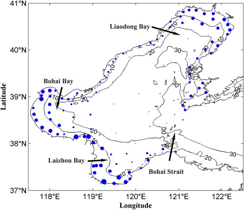
Fig. 1. Topography of the Bohai Sea (depth in meters) and routine monitoring stations (blue dots) in May, 2009. Dots represent the location of stations and the size of each dot indicates the relative concentration of total nitrogen (TN) in May, 2009.

2.3.2. Settings of the ocean pollutant transport model

Numerical experiments are performed to test the feasibility and reliability of the modified IPS when be applied to inversing the initial distribution of pollutant. The computing area is the Bohai Sea including the Liaodong Bay, the Bohai Bay, the Laizhou Bay and the central area. The integral time step length is 6 h and the total simulation time is 30 days.

3. IPS

The IPS is that the values of model parameters at some selected points, called independent points, are treated as independent variables and the values of model parameters at other points are obtained by interpolating the independent variables (Guo et al., 2017). It is a valid approach to reduce the quantity of variables that need to be inverted and promote the efficiency of the adjoint model, which has been shown by many previous works (Lu and Zhang, 2006; Fan and Lv, 2009; Zhang et al., 2011; Li et al., 2013; Wang et al., 2013; Chen et al., 2014; Zhang and Wang, 2014; Shen et al., 2015).

Determining an IPS means the determination of independent points and interpolation method. For independent points, there are two ways to select: uniformly in study area or according to the situation of the study. These two ways were both applied and contrasted by Lu and Zhang (2006), and their results demonstrated that it is better to select independent points according to the specific situation. As a result, the eight independent points are selected according to the observed distribution of the pollutant and the real topography of study area. In this section, the details of selection independent points and the introduction of the SSI are described.

3.1. Independent points

The Bohai Sea is surrounded by land on three sides, and the Bohai Strait is the only channel on the east side with the Yellow Sea. So, the ability of water exchange of the Bohai Sea is weak (Wang et al., 2013). In addition, there are three river systems – the Yellow River, Haihe River and Liaohe River – along the coast of the Bohai Sea, and they all discharge into the Bohai Sea with domestic and industrial wastewater. Therefore, the wastewater from those rivers is main source of pollution in the Bohai Sea.

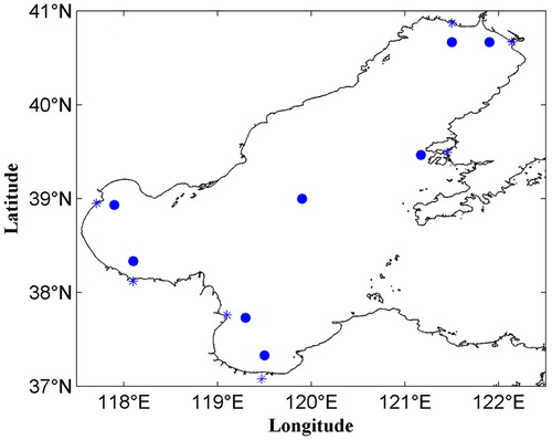
The observed pollutant concentration in Fig. 1 demonstrates that. The dots of Fig. 1 represent the location of routine monitoring stations and the size of each dot indicates the relative concentration of total nitrogen (TN). And concentration is high in three bays and the west of the Liaodong Peninsula, while low in the centre of the Bohai Sea. It is obvious that areas of high concentration are close to estuaries. As a result, seven independent points are selected firstly according to the pollutant distribution shown in Fig. 1 – two points in each bay, and one to the west of the Liaodong Peninsula. Also, the seven independent points are close to the estuary of Wei River, Yellow River, Tuhai River, Hai River, Daling River, Liao River and Fuzhou River, respectively (Fig. 2). In the process of confirming the location of seven independent points, what is considered is that the water flow of rivers and the relative locations of river estuaries in three bays. After that the eighth independent point is set in the centre of the Bohai Sea in order to ensure interpolation precision. The quantity and general location of independent point are confirmed by the above analysis, then a group experiments are carried out to determine the exact location of independent point. Finally, the most appropriate independent points are used in following numerical experiments.

Fig. 2. Locations of independent points. Dots represent independent points and stars represent estuaries.

3.2. SSI

CI is the main method in previous works and its formulation can be found in Li et al. (2013). Following Harder and Desmarais (1972), the SSI can be written as: (8) $$C_{i,j}={\displaystyle \sum _{k=1}^N{A}_k}\left(\frac{r_{i,j,k}^2}{R^2}\ln \frac{r_{i,j,k}^2}{R^2}+1-\frac{r_{i,j,k}^2}{R^2}\right)$$(8) where C_i,j represents TN concentration at the grid point (i, j); N is the total number of independent points; r_{i, j, k} represents the distance between the grid point (i, j) and the kth independent point; R is an influence radius, and A_k is the coefficients to be determined. In order to determine it, concentrations at independent points are substituted into Equation (8)(8) $$C_{i,j}={\displaystyle \sum _{k=1}^N{A}_k}\left(\frac{r_{i,j,k}^2}{R^2}\ln \frac{r_{i,j,k}^2}{R^2}+1-\frac{r_{i,j,k}^2}{R^2}\right)$$(8) , yielding (9) $$AX=C$$(9) (10) $$A={\left(A_1,A_2,\dots ,A_N\right)}^T$$(10) (11) $$C={\left(C_1,C_2,\dots ,C_N\right)}^T$$(11) (12) $$X=\left[\begin{array}{ccccc}1& w_{1,2}& \cdots & w_{1,(N-1)}& w_{1,N}\\ w_{1,2}& 1& \cdots & w_{2,(N-1)}& w_{2,N}\\ ⋮& ⋮& \ddots & ⋮& ⋮\\ w_{1,(N-1)}& w_{2,(N-1)}& \cdots & 1& w_{(N-1),N}\\ w_{1,N}& w_{2,N}& \cdots & w_{(N-1),N}& 1\end{array}\right]$$(12) where $C_1,C_2,\dots ,C_N$ are values at independent points, X is calculated according to the $r_{i,j,k}^2/R^2\ln r_{i,j,k}^2/R^2+1-r_{i,j,k}^2/R^2$ in Equation (8)(8) $$C_{i,j}={\displaystyle \sum _{k=1}^N{A}_k}\left(\frac{r_{i,j,k}^2}{R^2}\ln \frac{r_{i,j,k}^2}{R^2}+1-\frac{r_{i,j,k}^2}{R^2}\right)$$(8) , so $w_{i,j}=r_{i,j}^2/R^2\ln r_{i,j}^2/R^2+1-r_{i,j}^2/R^2$, and $r_{i,j}$ is the distance between the ith independent point and the jth independent point. Denoting D = X^–1, A_k can be derived as $A_k\text{=}{\displaystyle {\sum }_{kk=1}^N{C}_{kk}{D}_{k,kk}}$. Then (13) $$C_{i,j}={\displaystyle \sum _{kk=1}^N{\varphi }_{i,j,kk}{C}_{kk}}$$(13) where C_kk is the value at the kkth independent point, and ${\varphi }_{i,j,kk}$ is the interpolation coefficient of the kkth independent point at the grid point (i, j): (14) $${\varphi }_{i,j,kk}={\displaystyle \sum _{k=1}^N{D}_{k,kk}}\left(\frac{r_{i,j,k}^2}{R^2}\ln \frac{r_{i,j,k}^2}{R^2}+1-\frac{r_{i,j,k}^2}{R^2}\right)$$(14)

The TN concentration value at any other grid point can be obtained through interpolating values at independent points. Therefore, the optimization at all grid points can be achieved through optimizing values at independent points, which effectively reduces the number of variables that need to be inverted. Optimization of values at independent points can be realized through the following steps.

The gradient of cost function with respect to concentration values at independent points is calculated as: (15) $$\frac{\partial J}{\partial C_{kk}^1}={\displaystyle \sum _{kk=1}^N{\varphi }_{i,\hspace{0.17em}j,\hspace{0.17em}kk}\left(M+N+P\right)}$$(15) (16) $$M={\left(\frac{\partial C_{i,j}^{*}}{\partial t}\right)}^1$$(16) (17) $$N={\left(\frac{\partial (u_{i,\hspace{0.17em}j}{C}_{i,\hspace{0.17em}j}^{*})}{\partial x}\right)}^1+{\left(\frac{\partial (v_{i,\hspace{0.17em}j}{C}_{i,\hspace{0.17em}j}^{*})}{\partial y}\right)}^1+{\left(\frac{\partial (w_{i,\hspace{0.17em}j}{C}_{i,\hspace{0.17em}j}^{*})}{\partial z}\right)}^1$$(17) (18) $$P=\frac{\partial }{\partial x}{\left(K_H\frac{\partial C_{i,j}^{*}}{\partial x}\right)}^1+\frac{\partial }{\partial y}{\left(K_H\frac{\partial C_{i,j}^{*}}{\partial y}\right)}^1+\frac{\partial }{\partial z}{\left(K_V\frac{\partial C_{i,j}^{*}}{\partial z}\right)}^1$$(18) where the superscript 1 denotes the initial value, and the values at independent points are optimized by (19) $$C_{kk}=\stackrel{\wedge }{C_{kk}}-\frac{1}{K}\frac{\partial J}{\partial C_{kk}^1}$$(19) where C_kk is the value at the kkth independent point after optimization, $\stackrel{\wedge }{C_{kk}}$ is the one given based on experience, and the constant K is set as 1.4 × 10⁻⁶.

4. Numerical experiments and results

4.1. Ideal experiments

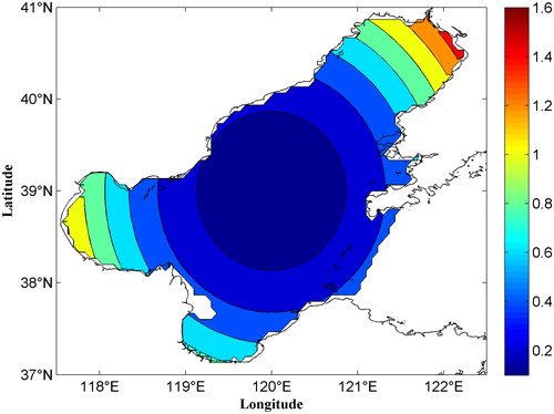
4.1.1. Description of ideal experiments. To testify the effectiveness and validity of SSI, the modified IPS is applied in ideal experiments. For the comparison, the previous IPS containing CI and same independent points with the modified IPS is also used. In these ideal experiments, we assume the initial distribution of TN concentration as a parabolic surface with downward convex just as shown in Fig. 3, which is prescribed based on the fact that the TN concentration is high in the coastal area and low in the centre of the Bohai Sea (Fig. 1). The forward model is run with the prescribed TN concentration as the initial background field and the simulation results at routine monitoring stations are taken as the ‘observations’. Then, the forward model is run again with a constant concentration as an initial guess value, and the difference in the concentration between simulated values and ‘observations’ at routine monitoring stations serves as the external force of the adjoint model. For reducing the difference, the initial guess value is adjusted using the steepest descent method, which is written as follows: (20) $$p^{k+1}=p^k-\alpha \cdot \nabla J\left(p\right)$$(20) where p is the parameter which is given an initial guess value and adjusted, $\nabla J\left(p\right)$ is the gradient of cost function with respect to this parameter, $\alpha$ is step length of the steepest descent method, and k is iteration steps of the adjoint method. By assimilating those ‘observations’, the initial guess value will be optimized, and the difference can be reduced continuously. Finally, the ‘optimal’ initial condition can be acquired.

Fig. 3. Assumed distribution of TN concentration (mg/L) in the Bohai Sea in ideal experiments.

The number of iteration steps of assimilation has a great impact on the inversion results, which depends on many factors, such as the initial guess value and the magnitude of smoothness (Wang et al., 2016). A good method for the confirmation of iteration steps is provided by Wang et al. (2016). Through trial and error, 50 iteration steps are determined based on the method. In this article, the iteration steps are same for all numerical experiments.

4.1.2. Results of ideal experiments

The normalized cost function (NCF) and mean absolute error (MAE) are significant assessment criteria for the validity of adjoint method. Figure 4 shows changes of NCFs against iterations (Fig. 4a), MAEs between simulated values and ‘observation’ at routine monitoring stations (MAE1) (Fig. 4b) and MAEs between the inverted values and prescribed ones at all grid points in the computing area (MAE2) (Fig. 4c) by two interpolation methods, CI and SSI, respectively.

Fig. 4. Results of ideal experiments. (a) The Normalized cost functions (NCFs), (b) mean absolute errors between simulated values and ‘observation’ at routine monitoring stations (MAE1) and (c) mean absolute errors between the inverted values and prescribed ones at all grid points in the computing area (MAE2s). Note that, in all panels, the blue solid lines are results by the Cressman interpolation (CI) and the red dashed lines are by the surface spline interpolation (SSI).

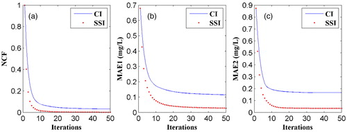
From Fig. 4a, it is found that the NCF tends to be stable after 10 iterations, and reach its minimum after 50 iterations by the two interpolation methods. There is no much changes for the NCFs between 10 and 50 iterations, which indicates the number of iterations steps selected in Section 4.1.1 is appropriate and too many iterations steps will cause the waste of computing resources. MAE1s and MAE2s shown in Fig. 4b,c reveal the proximity between inverted values and real values at routine monitoring stations and all grid points in the computing area, respectively. By the iteration, MAE1s and MAE2s both have dramatic declines, and it can be deduced that the assumed distribution of TN concentration has been inverted successfully.

The blue solid lines represent inverted results by the CI and the red dashed lines are by the SSI in Fig. 4, respectively. Values of red dashed lines after 50 iterations are all less than those of blue solid lines, which preliminarily displays the inverted results by the SSI are better than by the CI. Moreover, the NCFs at the last iteration step, and the MAEs between the simulated values and prescribed values are shown in Table 1, which gives more details of the inversion comparison between the CI and SSI. The MAE1 is reduced to 0.028 mg/L by the SSI and 0.086 mg/L by the CI, and the reductions are 95.9% and 87.4% after 50 iterations, respectively. For the MAE2, it is reduced to 0.034 mg/L by the SSI and 0.116 mg/L by the CI, which are reductions of 96.1% and 86.8%. Improvements by the SSI are 8.5% and 9.3% in terms of MAEs, and these comparisons quantitatively demonstrate that the accuracy of inversion results could be promoted by the SSI instead of the CI.

Table 1. Normalized cost functions (NCFs), mean absolute errors between simulated values and ‘observation’ at routine monitoring stations (MAE1s) and the mean absolute errors between the inverted values and prescribed ones at all grid points in the computing area (MAE2s) by the Cressman interpolation (CI) and the surface spline interpolation (SSI) in ideal experiments, respectively.

		MAE1 (mg/L)		MAE2 (mg/L)
Interpolation method	NCF	Initial	Final	Initial	Final
CI	2.0 × 10^−2	0.680	0.086	0.874	0.116
SSI	2.4 × 10^−3	0.680	0.028	0.874	0.034

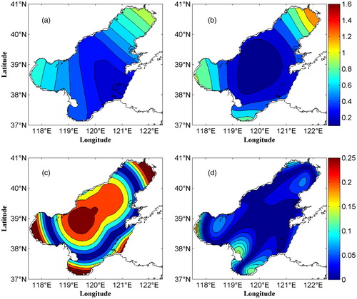
The comparison of distribution inverted by two interpolation methods are depicted in Fig. 5. Figure 5a,b show the distribution inverted by the CI and SSI, respectively. For the two figures, TN concentrations are low in the centre and high in the three bays, which is similar to the assumed initial distribution shown in Fig. 3. However, by contrasting them with the assumed initial distribution, it can be found that the inverted distribution by the SSI (Fig. 5b) is closer to the assumed than by the CI (Fig. 5a) in terms of the shape of distribution. Figure 5c,d are the absolute errors between the inverted initial distribution and the prescribed by the CI and SSI, respectively, which is more convenient to compare inversion results by two interpolation methods. It is obvious that the absolute errors by the SSI are less than those by the CI, and that is to say the distribution inverted by the SSI is closer to the assumed distribution in terms of the magnitude of TN concentrations.

Fig. 5. Results of ideal experiments. (a, b) The inverted initial distributions, (c, d) the absolute errors between the inverted initial distribution and the assumed shown in Fig. 3 (mg/L). Note that, (a, c) are results by the CI and (b, d) are those by the SSI.

Through ideal experiments, the effectiveness and advantage of the SSI over the CI are verified by lower MAEs and better similarity of inverted initial distribution to the prescribed.

4.2. Sensitivity experiments

In ideal experiments, ‘observations’ are obtained through strict mathematical calculation, meaning that there is no error in ‘observations’. But we all know that the practical in situ observations contain noises definitely. Thus, as sensitivity tests, artificial errors are added into ‘observations’, which are 10%, 50% and 80% of the accurate ‘observations’, respectively. Those noisy ‘observations’ are used instead of the error free ones, and then repeat above ideal experiments.

Using two interpolation methods, initial distribution inverted by assimilating ‘observations’ containing errors are shown in Fig. 6. Figure 6a,b is inverted by assimilating ‘observations’ containing 10% errors. The results inverted by assimilating ‘observations’ containing 50% errors are shown in Fig. 6c,d, and the other one are shown in Fig. 6e,f. Among these figures, Fig. 6a,c,e is inverted by the CI, and Fig. 6b,d,f is inverted by the SSI. From Fig. 6a,c,e or Fig. 6b,d,f it can be found that the basic structure that the concentration is low in centre and high in surroundings is basically unchanged, but the differences between the inversion results and the assumed distribution increase with the errors, no matter which interpolation method is. In addition, the distributions inverted by the SSI are more similar to the assumed than by the CI for the three percentage errors. The MAE2s of the sensitivity experiments are calculated and shown in Table 2, which all increase with the percentage errors. But it is important that the MAE2 by the SSI is lower than that by the CI no matter which the error is. Even, the MAE2 by the SSI in the case containing 10% errors is smaller than that by the CI in the case of containing 0 error. This quantitative comparison shows the advantage of the SSI at the interpolation accuracy. This result is consistent with the conclusion from Fig. 6.

Fig. 6. Inverted initial distributions of sensitivity experiments. (a, b) Inverted by assimilating ‘observations’ containing 10% errors, (c, d) containing 50% errors, (e, f) contains 80% errors. Note that, (a, c, e) are inverted by the CI and (b, d, f) are by the SSI.

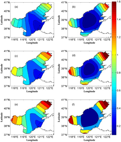
Table 2. MAE2s by the CI and the SSI through assimilating ‘observations’ containing with percentage errors in sensitivity experiments, respectively.

	MAE2 (mg/L)
Percentage errors	CI	SSI
0	0.116	0.034
10	0.180	0.057
50	0.308	0.221
80	0.442	0.352

In sensitivity experiments, the SSI has a better performance in terms of the inverted TN concentration distribution and MAE than the CI when assimilates inaccurate ‘observations’, which demonstrates the reliability of the SSI and it is more suitable for the application in practical experiments.

4.3. Practical experiments

The advantage of the SSI is presented through the comparisons with the CI in ideal and sensitivity experiments, and then this interpolation method is implemented with both the real position and values of routine monitoring stations depicted in Fig. 1 in this section.

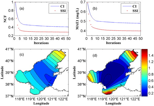
The variations of NCF (Fig. 7a) and MAE1s (Fig. 7b) with iterations and the initial distributions of TN concentrations (Fig. 7c,d) inverted by two interpolation methods are shown in Fig. 7. Both the NCF and MAE1 display great declines through iteration, which demonstrates the effectiveness of the adjoint method. Moreover, the lower MAE1 displays the improvement of precision by the SSI, again. Figure 7c,d are initial distributions inverted by the CI and SSI, respectively. The concentrations are low in the centre of the Bohai Sea in these two figures, but the strip distribution of Fig. 7c is conflictive with the observed distribution shown in Fig. 1. In addition, from Fig. 1 it can be found that the concentration of pollutant is reduced gradually from coast to open-sea in three bays. However, the concentration is uniform in the Bohai Bay and Laizhou Bay in Fig. 7c, which is incompatible with the observed phenomenon in Fig. 1. But, this phenomenon is reproduced by applying the SSI, and the highest concentration appears in the coastal areas. That is reasonable because the pollutant is discharged into the Bohai Sea through rivers.

Fig. 7. Results of practical experiments. (a) The NCFs, (b) the MAE1s, (c) the initial distribution inverted by the CI, (d) the initial distribution inverted by the SSI.

In view of the inversion distributions by two interpolation methods in three bays, the comparisons highlight the differences in these places, and the MAE1 in each bay is calculated and listed in Table 3. The BHB, LDB and LZB represent the MAE1 in the Bohai Bay, the Liaodong Bay and the Laizhou Bay after 50 iterations, respectively. It can be found that the MAE1s by the SSI are lower than by the CI in all three bays, and the maximal improvement by applying the SSI is 36% in the Liaodong Bay and the minimal is 15% in the Bohai Bay. No matter how the improvement is, it will appear as long as the SSI is applied. As a result, the application of SSI brings meaningful improvement under other same conditions.

Table 3. MAE1s by the CI and the SSI in practical experiments, respectively.

	MAE1 (mg/L)
Interpolation method	BHB	LDB	LZB
CI	0.450	0.259	0.500
SSI	0.382	0.166	0.405

The BHB, LDB, and LZB represent the MAE1 in the Bohai Bay, the Liaodong Bay and the Laizhou Bay after 50 iterations, respectively.

In practical experiments, the comparisons of SSI and CI are displayed through the inverted distributions and MAEs in three bays. The more reasonable inverted distribution and the reduced error indicate that the application of SSI causes meaningful and comprehensive improvements.

5. Discussion

For acquiring a good initial condition, an appropriate interpolation is the crucial factor, and the application of SSI further improves the accuracy of the inverted initial condition. In fact, the advantage of SSI has been identified by many previous works. The comparison with 4-nearest neighbours method was tested by Perrin et al. (1987), and their results revealed that spline method improves smoothness and gives more precisely located extrema. They also indicated that surface splines are differentiable and faster at the rates of convergence toward the ‘true’ potential surface. The similar comparison can be found in Wijnands et al. (2016). They developed a new model for near-surface wind speeds in tropical cyclones based on the spline interpolation, which yields more accurate modelling in the area of maximum winds.

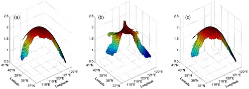
The spline is a special function that defined piecewise by polynomials, so it is good at smoothing in nature. Pan et al. (2017) contrasted the spline interpolation, the CI and the kriging interpolation through a curve interpolation experiment, and their results showed that the curve obtained with the spline interpolation is smooth and very close to the original curve. Similarly, in order to reveal the natural advantage of the SSI in the accuracy and smoothness of interpolation result, a simple interpolation experiment is implemented and the result is shown in Fig. 8. In this experiment, a surface is prescribed (Fig. 8a) and the above eight independent points are used. Moreover, the values of the eight points on the surface are known. Then, the interpolation is implemented based on the eight known points by the CI and SSI, respectively. Figure 8b,c are the interpolation results by the CI and SSI, respectively. Obviously, the result by the SSI is much better than the result by the CI at the accuracy and smoothness. The MAE between interpolation results and the prescribed are 0.0352 and 0.1293 by the SSI and CI, respectively. It can be concluded that the SSI is better than CI at surface interpolation in nature. Therefore, the SSI has a better performance than CI in numerical experiments of Section 4.

Fig. 8. Comparison of the interpolation results by the CI and SSI. (a) The prescribed surface, (b) the interpolation result by the CI, (c) the interpolation result by the SSI.

In addition, the inversion results are also influenced by the number of independent points besides the interpolation method. This factor has been discussed by Wang et al. (2013), in which more than one hundred independent points are used. However, only eight independent points are used based on the application of SSI in this article. More importantly, under the same assumed initial distribution of TN concentration, the MAE is 0.06 mg/L in Wang et al. (2013), larger than 0.03 mg/L of this work. Through applying the SSI, the quantity of independent points is reduced, and the precision is improved.

As a result, the application of SSI provides a more smoothness, accuracy and reasonableness inversion result, which also reduces the quantity of independent points and variables that need to be inverted, and improves the computational efficiency of the adjoint model.

6. Summary

More attentions have been paid to the diffusion of pollutant due to serious threats from human activities to marine ecosystem, and a better initial condition is needed for accurate prediction. The ocean pollutant transport model combined with IPS is a power tool to acquire an accurate initial condition. Based on the IPS, the influence of the interpolation method on the accuracy of initial condition must be considered. The CI is mainly used in IPS in pervious works, but its inverted result has inferior smoothness and large errors. On the contrary, the SSI could improve the smoothness of result and it has been used in many studies. As a result, the CI and the SSI are applied to inverting and contrasting the initial condition in the ocean pollutant transport model with the adjoint method.

In ideal experiments, MAE1 and MAE2 by the SSI are lower than those by the CI. Moreover, the initial distribution inverted by the SSI is also closer to the prescribed one. Those results indicate the effectiveness and advantage of SSI over CI. In sensitivity experiments, the MAEs by SSI are always lower than by CI no matter what the artificial error is, also, the distributions inverted by SSI are more similar to the prescribed. Results of the comparisons demonstrate the reliability of SSI. In practical experiments, MAE1s by the SSI are all lower than those by the CI in three bays, and more importantly, the initial distribution inverted by the SSI is more reasonable.

Results of numerical experiments certify the effectivity, reliability and reasonability of the SSI combined with IPS and adjoint method to invert the initial condition for the ocean pollutant transport model. It is worth to do more works based on the SSI.

Geolocation information

In this work, the study area is the Bohai Sea, which is the water west of the Bohai Strait (117.5°E–122.5°E, 37°N–41°N). Section 2.3.2 describes the Bohai Sea in more detail and it is shown in Fig. 1.

Acknowledgments

We gratefully acknowledge the support from Haidong Pan on the program of spline interpolation.

Disclosure statement

No potential conflict of interest was reported by the authors.

Additional information

Funding

This work was supported by the National Natural Science Foundation of China [Grant number 41606006] and the National Key Research and Development Plan [Grant number 2016YFC1402304].

References

- Arkhipov, B., Koterov, V., Solbakov, V., Shapochkin, D. and Yurezanskaya, Y. 2007. Numerical simulation of pollution and oil spill spreading by the stochastic discrete particle method. Comput. Math. Math. Phys. 47, 280–292. DOI:10.1134/S096554250702011X.
- Boehm, P., Murray, K. and Cook, L. 2016. Distribution and attenuation of polycyclic aromatic hydrocarbons in Gulf of Mexico seawater from the deepwater horizon oil accident. Environ. Sci. Technol. 50, 584–592. DOI:10.1021/acs.est.5b03616.
- Chen, H., Cao, A., Zhang, J., Miao, C. and Lv, X. 2014. Estimation of spatially varying open boundary conditions for a numerical internal tidal model with adjoint method. Math. Comput. Simul. 97, 14–38. DOI:10.1016/j.matcom.2013.08.005.
- Chen, H-Z., Li, D-M. and Li, X. 2007. Mathematical modeling of oil spill on the sea and application of the modeling in Daya Bay. J. Hydrodynam. 19, 282–291. DOI:10.1016/S1001-6058(07)60060-2.
- Correa, S., Araujo, J., Penha, J., Cunha, C., Stevenson, P. and co-authors. 2015. Overfishing disrupts an ancient mutualism between frugivorous fishes and plants in Neotropical wetlands. Biol. Conserv. 191, 159–167. DOI:10.1016/j.biocon.2015.06.019.
- Debreu, L., Marchesiello, P., Penven, P. and Cambon, G. 2012. Two-way nesting in split-explicit ocean models: algorithms, implementation and validation. Ocean Model. 49–50, 1–21. DOI:10.1016/j.ocemod.2012.03.003.
- Dimet, F. L. E. and Talagrand, O. 1986. Variational algorithms for analysis and assimilation of meteorological observations: theoretical aspects. Tellus A. 38, 97–110. DOI:10.3402/tellusa.v38i2.11706.
- Egbert, G. D. and Erofeeva, S. Y. 2002. Efficient inverse modeling of barotropic ocean tides. J. Atmos. Ocean. Technol. 19, 183–204. DOI:10.1175/1520-0426(2002)019<0183:EIMOBO>2.0.CO;2.
- Eyring, V., Köhler, H., Aardenne, J. and Lauer, A. 2005. Emissions from international shipping: 1. the last 50 years. J. Geophys. Res. 110, 3928–3950.
- Faghihifard, M. and Badri, M. 2016. Simulation of oil pollution in the Persian Gulf near Assaluyeh oil terminal. Mar. Pollut. Bull. 105, 143–149. DOI:10.1016/j.marpolbul.2016.02.034.
- Fan, W. and Lv, X. 2009. Data assimilation in a simple marine ecosystem model based on spatial biological parameterizations. Ecol. Model. 220, 1997–2008. DOI:10.1016/j.ecolmodel.2009.04.050.
- Guo, Z., Pan, H., Fan, W. and Lv, X. 2017. Application of surface spline interpolation in inversion of bottom friction coefficients. J. Atmos. Ocean. Technol. 34, 2021–2028. DOI:10.1175/JTECH-D-17-0012.1.
- Harder, R. and Desmarais, R. 17972. Interpolation using surface splines. J. Aircr. 9, 189–191. DOI:10.2514/3.44330.
- Huang, H., Chen, G. and Zhang, Q. 2010. The distribution characteristics of pollutants released at different cross-sectional positions of a river. Environ. Pollut. 158, 1327–1333. DOI:10.1016/j.envpol.2010.01.010.
- Kojima, K., Furumai, H., Hata, A., Kasuga, I., Kurisu, F. and co-authors. 2011. Monitoring and numerical simulation of pathogenic pollution after CSO event in coastal waters of Tokyo Bay. In: Proceedings of the 12th International Conference on Urban Drainage, Porto Alegre, 87–88.
- Lee, S., Wolberg, G. and Shin, S. 1997. Scattered data interpolation with multilevel B-splines. IEEE Trans. Vis. Comput. Graph. 3, 228–244. DOI:10.1109/2945.620490.
- Li, X., Wang, C., Fan, W. and Lv, X. 2013. Optimization of the spatiotemporal parameters in a dynamical marine ecosystem model based on the adjoint assimilation. Math. Probl. Eng. 2013, 1–12.
- Lu, X. and Zhang, J. 2006. Numerical study on spatially varying bottom friction coefficient of a 2D tidal model with adjoint method. Cont. Shelf. Res. 26, 1905–1923. DOI:10.1016/j.csr.2006.06.007.
- Meissa, B. and Gascuel, D. 2015. Overfishing of marine resources: Some lessons from the assessment of demersal stocks off Mauritania. ICES J. Mar. Sci. 72, 414–427. DOI:10.1093/icesjms/fsu144.
- Øyvind,, E., Eirik, S., Sundet, J., Dalsøren, S., Isaksen, I. and co-authors. 2003. Emission from international sea transportation and environmental impact. J. Geophys. Res. Atmos. 108, 129–144.
- Pan, H., Guo, Z. and Lv, X. 2017. Inversion of tidal open boundary conditions of the M2constituent in the Bohai and Yellow seas. J. Atmos. Ocean. Technol. 34, 1661–1672. DOI:10.1175/JTECH-D-16-0238.1.
- Paul, J. H., Hollander, D., Coble, P., Daly, K. L., Murasko, S. and co-authors. 2013. Toxicity and mutagenicity of Gulf of Mexico waters during and after the Deepwater Horizon oil spill. Environ. Sci. Technol. 47, 9651–9659. DOI:10.1021/es401761h.
- Peng, S. and Xie, L. 2006. Effect of determining initial conditions by four-dimensional variational data assimilation on storm surge forecasting. Ocean Model. 14, 1–18. DOI:10.1016/j.ocemod.2006.03.005.
- Penven, P., Debreu, L., Marchesiello, P. and McWilliams, J. C. 2006. Evaluation and application of the ROMS 1-way embedding procedure to the central California upwelling system. Ocean Model. 12, 157–187. DOI:10.1016/j.ocemod.2005.05.002.
- Perrin, F., Pernier, J., Bertnard, O., Giard, M. H. and Echallier, J. F. 1987. Mapping of scalp potentials by surface spline interpolation. Electroencephalogr. Clin. Neurophysiol. 66, 75–81. DOI:10.1016/0013-4694(87)90141-6.
- Sámano, M., Pérez, M., Claramunt, I. and García, A. 2016. Assessment of the zinc diffusion rate in estuarine zones. Mar. Pollut. Bull. 104, 121–128. DOI:10.1016/j.marpolbul.2016.01.052.
- Scholkmann, F., Spichtig, S., Muehlemann, T. and Wolf, M. 2010. How to detect and reduce movement artifacts in near-infrared imaging using moving standard deviation and spline interpolation. Physiol. Meas. 31, 649. DOI:10.1088/0967-3334/31/5/004.
- Shchepetkin, A. and McWilliams, J. 2005. The regional oceanic modeling system (ROMS): a split-explicit, free-surface, topography-following-coordinate oceanic model. Ocean. Model. 9, 347–404. DOI:10.1016/j.ocemod.2004.08.002.
- Shen, Y., Wang, C., Wang, Y. and Lv, X. 2015. Inversion study on pollutant discharges in the Bohai Sea with the adjoint method. J. Ocean Univ. China. 14, 941–950. DOI:10.1007/s11802-015-2501-8.
- Sidorovskaia, N., Ackleh, A., Tiemann, C., Ma, B., Ioup, J. and co-authors. 2016. Passive acoustic monitoring of the environmental impact of oil exploration on marine mammals in the Gulf of Mexico. Adv. Exp. Med. Biol. 875, 1007–1014. DOI:10.1007/978-1-4939-2981-8.
- Tappin, A., Burton, J., Millward, G. and Statham, P. 1997. A numerical transport model for predicting the distributions of Cd, Cu, Ni, Pb and Zn in the southern North Sea: the sensitivity of model results to the uncertainties in the magnitudes of metal inputs. J. Mar. Syst. 13, 173–204. DOI:10.1016/S0924-7963(96)00112-1.
- Walsh, J., Lenes, J., Darrow, B., Parks, A. and Weisberg, R. 2016. Impacts of combined overfishing and oil spills on the plankton trophodynamics of the West Florida shelf over the last half century of 1965–2011: A two-dimensional simulation analysis of biotic state transitions, from a zooplankton-to a bacterioplank. Cont. Shelf Res. 116, 54–73. DOI:10.1016/j.csr.2016.01.007.
- Walsh, J. J., Lenes, J. M., Darrow, B. P., Parks, A. A., Weisberg, R. H. and co-authors. 2015. A simulation analysis of the plankton fate of the Deepwater Horizon oil spills. Cont. Shelf Res. 107, 50–68. DOI:10.1016/j.csr.2015.07.002.
- Wang, C., Li, X. and Lv, X. 2013. Numerical study on initial field of pollution in the Bohai Sea with an adjoint method. Math. Probl. Eng. 4, 389–405.
- Wang, D., Cao, A., Zhang, J., Fan, D., Liu, Y., and co-authors. 2016. A three-dimensional cohesive sediment transport model with data assimilation: Model development, sensitivity analysis and parameter estimation. Estuar. Coast. Shelf. Sci. 206, 87–100.
- Wang, D., Zhang, J., He, X., Chu, D., Lv, X. and co-authors. 2018. Parameter estimation for a cohesive sediment transport model by assimilating satellite observations in the Hangzhou Bay: Temporal variations and spatial distributions. Ocean Model. 121, 34–48. DOI:10.1016/j.ocemod.2017.11.007.
- Wang, S., Shen, Y., Guo, Y. and Tang, J. 2008. Three-dimensional numerical simulation for transport of oil spills in seas. Ocean. Eng. 35, 503–510. DOI:10.1016/j.oceaneng.2007.12.001.
- Wei, L., Hu, Z., Dong, L. and Zhao, W. 2015. A damage assessment model of oil spill accident combining historical data and satellite remote sensing information: a case study in Penglai 19-3 oil spill accident of China. Mar. Pollut. Bull. 91, 258–271. DOI:10.1016/j.marpolbul.2014.11.036.
- Wijnands, J. S., Qian, G. and Kuleshov, Y. 2016. Spline-based modelling of near-surface wind speeds in tropical cyclones. Appl. Math. Model. 40, 8685–8707. DOI:10.1016/j.apm.2016.05.013.
- Xing, Q., Meng, R., Lou, M., Bing, L. and Liu, X. 2015. Remote sensing of ships and offshore oil platforms and mapping the marine oil spill risk source in the Bohai Sea. Aquat. Procedia. 3, 127–132. DOI:10.1016/j.aqpro.2015.02.236.
- Xu, M. and Chua, V. 2017. A numerical study on land-based pollutant transport in Singapore coastal waters with a coupled hydrologic-hydrodynamic model. J. Hydro-Environ. Res. 14, 119–142. DOI:10.1016/j.jher.2016.09.002.
- Yu, L. and O'Brien, J. J. 1992. On the initial condition in parameter estimation. J. Phys. Oceanogr. 22, 1361. DOI:10.1175/1520-0485(1992)022<1361:OTICIP>2.0.CO;2.
- Zhang, J. and Kitazawa, D. 2015. Numerical analysis of particulate organic waste diffusion in an aquaculture area of Gokasho Bay, Japan. Mar. Pollut. Bull. 93, 130–143. DOI:10.1016/j.marpolbul.2015.02.007.
- Zhang, J. and Lu, X. 2008. Parameter estimation for a three-dimensional numerical barotropic tidal model with adjoint method. Int. Int. J. Numer. Meth. Fluids. 57, 47–92. DOI:10.1002/fld.1620.
- Zhang, J., Lu, X., Wang, P. and Wang, Y. 2011. Study on linear and nonlinear bottom friction parameterizations for regional tidal models using data assimilation. Cont. Shelf Res. 31, 555–573. DOI:10.1016/j.csr.2010.12.011.
- Zhang, J. and Wang, Y. 2014. A method for inversion of periodic open boundary conditions in two-dimensional tidal models. Comput. Methods Appl. Mech. Eng. 275, 20–38. DOI:10.1016/j.cma.2014.02.020.