Adding new evidence to the attribution puzzle of the recent water shortage over São Paulo (Brazil)

Abstract

São Paulo, Brazil has experienced severe water shortages and record low levels of its water reservoirs in 2013–2014. We evaluate the contributions of Amazon deforestation and climate change to low precipitation levels using a modelling approach, and address whether similar precipitation anomalies might occur more frequently in a warming world. Precipitation records from INMET show that the dry anomaly extended over a fairly large region to the north of São Paulo. Unique features of this event were anomalous sea surface temperature (SST) patterns in the Southern Atlantic, an extension of the sub tropical high into the São Paulo region and moisture flux divergence over São Paulo. The SST anomalies were very similar in 2013/14 and 2014/15, suggesting they played a major role in forcing the dry conditions. The SST anomalies consisted of three zonal bands: a cold band in the tropics, a warm band to the south of São Paulo and another cold band poleward of 40 S. We performed ensemble climate simulations with observed SSTs prescribed, vegetation cover either fixed at 1870 levels or varying over time, and greenhouse gases (GHGs) either fixed at pre-industrial levels (280 ppm CO₂) or varying over time. These simulations exhibit similar precipitation deficits over the São Paulo region in 2013/14. From this, we infer that SST patterns and the associated large-scale state of the atmosphere were important factors in determining the precipitation anomalies, while deforestation and increased GHGs only weakly modulated the signal. Finally, analyses of future climate simulations from CMIP5 models indicate that the frequency of such precipitation anomalies is not likely to change in a warmer climate.

Keywords:

• water shortages
• deforestation
• pattern recognition algorithm
• climate change
• sea surface temperature anomaly

1. Introduction

São Paulo, Brazil is the largest metropolitan region of the Southern Hemisphere with a population of about 20 million (United Nations Department of Economic and Social Affairs Population Division, 2015). This region receives most of its precipitation during austral summer (October–March) with a peak during December–February (DJF) and experiences a usually well-defined dry period during the austral winter (Barros et al., 2000). The Cantareira reservoir system is the largest source of water for São Paulo’s metropolitan region, which under normal conditions supplies water to 8.8 million people. Records from the utility company of São Paulo (SABESP - COMPANHIA DE SANEAMENTO BÁSICO DO ESTADO DE SÃO PAULO, 2008) reveal that the Cantareira reservoir system which has been in operation since 1976 reached the lowest historical water level in 2014/15 (Coutinho et al. 2015; Otto et al., 2015; Nobre et al., 2016) causing a severe water shortage in the region. This water shortage led to a number of impacts in several socioeconomic sectors such as water availability for human consumption, irrigation, hydropower generation, food and energy production (King et al. 2015; Munich, 2015; Swiss-Re 2015; UNICA, 2015). For future planning of water provision to São Paulo, it is therefore important to understand the various causes of the extremely low reservoir levels and evaluate the risk of future water shortage.

The state of São Paulo experienced a persistent rainfall deficit during the period from 2012 to 2015, with particularly low precipitation during the DJF 2013/14 wet season (Coelho et al., 2016a; Nobre et al., 2016). These conditions contributed to the low levels of the reservoir system. The precipitation deficit extended not only over the state of São Paulo but also over the whole southeast of Brazil (Seth et al., 2015; Coelho et al. 2016a, b; Getirana 2016; Cavalcanti et al. 2017). The general climate constellation during the 2013–14 wet season (DJF) has been analysed by Coelho et al. (2016a, b) in detail. In brief, the South Atlantic subtropical high extended anomalously far to the west during this period. The high-pressure zone was maintained over an anomalously warm sea surface temperature (SST) region in the southwestern South Atlantic. This system contributed to the observed precipitation deficit over southeast Brazil. The system was also associated with a reduction in the number of ‘South Atlantic convergence zone’ (SACZ) episodes. The SACZ is an elongated convective band originating in the Amazon basin, extending south-eastwards across southeast Brazil into the subtropical Atlantic Ocean (Kodama, 1993; Herdies et al., 2002, Carvalho et al., 2004; Kolusu et al. 2015; Otto et al., 2015; Seth et al., 2015; Silva et al., 2015; Nobre et al., 2016). According to these studies the regular humidity transport from the Amazon region that normally reaches the southeast region of Brazil during SACZ episodes, was directed towards southern Brazil instead. Indeed, during January 2014, an anti-cyclonic anomaly was established over most of subtropical South America east of the Andes, which weakened the SACZ activity. As a result of this, drought conditions occurred in Southeastern Brazil in summer of 2014 (Espinoza et al., 2014; Nobre et al 2016). In parallel to the drought over the Sao Paulo region, very strong precipitation anomalies occurred in Western Amazonia (Nobre et al., 2016).

Coelho et al. (2016a), Otto et al. (2015) and Coutinho et al. (2015) have also investigated to what extent the climate anomaly in December 2013 to February 2014 and over the extended January 2014 to February 2015 period was extraordinary by comparing the precipitation anomalies with historical precipitation records. Their study found that the 2013/14 austral summer was exceptionally dry over the São Paulo region. Dry events had been recorded previously, but the precipitation deficit was smaller. Cavalcanti et al. (2017) found that there was an opposite precipitation signal in the western Amazon (very wet) to that in southeast Brazil (very dry), in January 2014 and 2015. Getirana (2016) studied the extreme water deficit in Brazil using satellite data. He found a reduction of 20–23% of precipitation over an extended period of 3 years. The rainfall deficit over southeast Brazil is also positively correlated with the warm SST over the equatorial western Pacific Ocean (Espinoza et al., 2014; Coelho et al., 2016b; Cavalcanti et al., 2017) and negatively correlated with equatorial central Pacific Ocean (Coelho et al., 2016b). Coelho et al. (2016b) also found a large scale teleconnection pattern between 200 hPa geopotential height and Indonesian heat source.

Given the vital role of water, it is important to understand in full the causes of the shortage. A range of popular articles both in newspapers and science journals have created the impression that deforestation may have contributed to the Sao Paulo drought (Escobar, 2015; Nazareno and Laurence, 2015) and led to studies addressing this question (Marengo and Alves, 2015). Another hypothesis is that global warming due to greenhouse gas (GHG) emissions to the atmosphere may have affected the tropical hydrological cycle, and in the future more such events may occur (Escobar, 2015). In order to contribute to the São Paulo water shortage attribution problem, this article aims to address the following questions using observations and model simulations: (1) What is the likely contribution of Amazon deforestation to the anomalies? (2) Is there a likely link between the drought events and climate change? (3) Are 2013/14 conditions likely to occur more frequently in the future?

We first re-examine the 2013/14 water shortage event, thereby expanding on the analysis of Coelho et al. (2016b), to establish to what extent and in which way the 2013/14 event was anomalous. We then use various ensemble simulations with an atmospheric general circulation model (AGCM) forced with observed SSTs (as compiled by HadISST [Rayner et al., 2003]), to study the contribution of land use cover change (LUCC) and elevated GHG levels on the rainfall anomalies over the São Paulo region. Finally, we use a pattern recognition approach to investigate whether climate models project a future increase in the precipitation deficit of the type observed during 2013/14, i.e. indirectly whether climate change would increase pressure on water supply via an increase of droughts. The data and experimental design are described in Section 2. Section 3 presents the results and a discussion, and conclusions are presented in Section 4.

2. Data and methods

For our study we used multiple observational datasets and factorial model simulations. Rainfall anomalies were investigated using station-based records from the Brazilian National Meteorological Service (INMET) and the Global Historical Climatology network (Peterson and Vose, 1997; available at http://www.ncdc.noaa.gov/ghcnm/v2.php), and precipitation estimates from gridded datasets from the Global Precipitation Climatology Project (GPCP; Adler et al., 2003). In this study, three INMET stations, Guarulhos, Taubate and Catanduva, have been considered (Fig. 1a). There are also station data available for Mirante de Santana from INMET and Parque Estadual das Fontes do Ipiranga from Universidade De São Paulo (USP) located inside São Paulo City, which show very different trends from the sites outside the city, but we refrained from relying on these two records because they are not located in the catchment area of the reservoirs and because it is likely that they are affected by the so-called ‘urban rainfall effect’. Indeed large urban areas have been shown to affect downwind rainfall, leading to average increases of 28% (Shepherd et al., 2002) and it seems very difficult to separate these effects in precipitation records from larger-scale effects. The Cantareira reservoir water volume data were obtained from the water and waste management company of São Paulo state SABESP (Companhia de Saneamento Básico do Estado de São Paulo S.A.), moisture transport and mean sea level pressure were obtained from the European Centre for Medium-Range Weather Forecasts (ECMWF) Reanalysis Interim (ERA-Interim; Dee et al., 2011). ERA-Interim combines observations and model output to obtain a best estimate of historical climate. It covers the period from 1 January 1979 to present day.

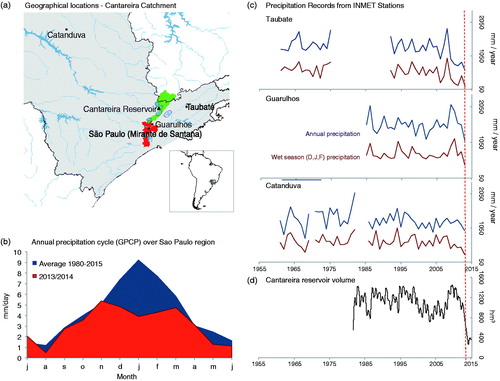
Fig. 1. (a) Geographical location of the São Paulo Cantareira water reservoir and the INMET climate stations in São Paulo State, (b) annual cycle of rainfall for 2013/14 and long-term mean for the period 1979–2004 from GPCP over São Paulo (averaged over the region 50°W to 45°W and 25°S to 20°S), (c) water storage volume (hm³) of Cantareira reservoir system for the period 1982 to early 2015 and (d) annual (July–June) and wet season (December, January and February) rainfall measured at the INMET stations in the State of São Paulo from 1961 to 2014.

To probe the effect of changes in land use cover and GHG levels on the observed climate anomalies, we performed simulations using the atmospheric component of the Hadley Centre Climate model (HadAM3; Pope et al., 2000). We chose this setup because it permits us to impose observed SSTs and make comparisons with observations. Previously, several researchers have validated the HadAM3 model for the present climate over South America (Chou et al., 2012; Reboita et al., 2014; Cabré et al., 2016) and found that the model performs well. We have also investigated the different aspects of model performance that are important for simulating the 2013/14 anomalies according to previous studies. Specifically, model 200 hPa geopotential height captures the large-scale teleconnection pattern associated with an Indonesian upper troposphere heat source, as described in Coelho et al. (2016b), although it was somewhat displaced to the west when compared with the observed pattern, particularly the low pressure anomaly over southern south America, and magnitudes were also lower. Furthermore, the geopotential-height anomaly at 200 hPa over the Atlantic near the southeast Brazil region where the blocking system manifested itself and contributed to the precipitation deficit was well reproduced in the simulation in each of the summer months in 2013/14 (see Supplementary Fig. S1).

For all simulations we prescribed SSTs and sea ice from 1850 to 2016 from the Hadley Centre Global Sea Ice and Sea Surface Temperature (HadISST) datasets (Rayner et al., 2003). With these boundary conditions fixed we performed three simulation scenarios (see Table 1)

1. Fixed land cover as in 1870 following Meiyappan and Jain (2012) and fixed GHG levels at preindustrial values (i.e. CO₂ fixed to 280 ppm),

2. Time varying land cover using the reconstruction of Meiyappan and Jain (2012) and fixed pre-industrial GHG levels, and

3. Time varying land cover and time-varying atmospheric GHG levels following observations.

Table 1. Simulations carried out with HadAM3.

Simulation scenarios	Number of ensembles	SST	GHG	Land cover
1	6	Observed SST (HadISST)	Fixed at pre-industrial (280 ppm)	Fixed at 1870
2	6	Observed SST (HadISST)	Fixed at pre-industrial (280 ppm)	Time varying land cover (Meiyappan and Jain, 2012)
3	31	Observed SST (HadISST)	Increasing CO2	Time varying land cover (Meiyappan and Jain, 2012)

LUCC between 1870 and 2013 from reconstructions by Meiyappan and Jain (2012) reveal a reduction in the fraction of broad leaf trees at the cost of grasses towards southeast Brazil (see Supplementary Fig. S2).

For each of these scenarios we first run one complete simulation starting in the year 1870 and ending in 2015. Because of the chaotic nature of the atmospheric circulation we then produce ensembles based on slightly different initial conditions by slightly varying the time-step for updating vegetation cover or slightly shifting the start date. For creating these ensembles, we restart the simulations in 1970. For the first two scenarios (fixed vegetation and fixed GHG levels and observed changing land cover and fixed GHG levels) we created ensembles of 5 simulations while for the third scenario (changing land cover and changing GHG levels) we created a larger ensemble with 5 ensemble members starting in 1970 and 25 additional ones in 2008. We chose this large ensemble for the third scenario because it should be the most realistic and thus we wanted to improve statistical power for this case.

In order to assess the occurrence frequency of anomalous precipitation patterns similar to 2013/14 in the future, we use projections from the Fifth Coupled Model Inter-comparison Project (CMIP5, Taylor et al., 2012) with three well-established climate models listed in Table 2 forced with the Representative Concentration Pathways (RCPs) 8.5 scenario. This scenario is a high emissions scenario, which reaches an atmospheric CO₂ level of 900 ppm by 2100.

Table 2. List of CMIP5 climate models and ensemble outputs used in this study, simulation period, and research groups responsible for their development.

Models	Reference	Simulation period
CCSM4	Gent et al. (2011)	Jan 1850–Dec 2300
GFDL-ESM2M	Dunne et al. (2012, 2013)	Jan 1861–Dec 2100
HadGEM2-ES	Collins et al. (2011)	Dec1859–Dec 2299

3. Results and discussion

3.1 Evidence of water shortage based on observed and reanalysis datasets

3.1.1 Local precipitation and reservoir level records

We first briefly review what in-situ historical precipitation records from INMET tell us about the 2013/14 event (stations shown in Fig. 1a). An advantage of these records over gridded datasets is that they do not involve any interpolation or extrapolation. On the other hand, a disadvantage is that the records are not continuous. Total annual rainfall has been calculated as the sum of rainfall from July to June of the following year for each year from 1961 to 2014 (Fig. 1c). The observed rainfall during DJF 2013/14 was reduced by 86% at Taubate, and by 40–50% at the Guarulhos and Catanduva station with respect to the 1961–2014 mean (Fig. 1c). The precipitation records from these three stations, including Cantanduva, which is located farther away in the northwest of the reservoir (Fig. 1a), show that the dry anomaly extended over a fairly large region. Thus the observed precipitation deficit 2013/14 was not just restricted to the close vicinity of São Paulo city but was of a larger-scale regional character. The annual cycle of rainfall for 2013/14 and long-term mean from GPCP (Fig. 1b) over this larger region (averaged over the region 50°W to 45°W and 25°S to 20°S), clearly shows that the precipitation reduction occurred during the peak rainy season (i.e. December 2013 to February 2014). In these three months, the precipitation was reduced by more than 50% in each of the months.

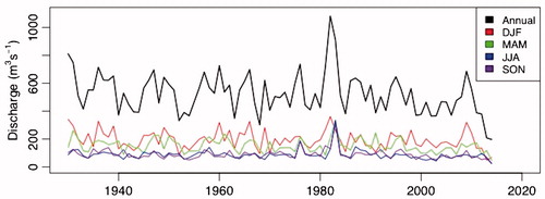
For completeness we also reproduce here the time series of reservoir water storage volume from Companhia De Saneamento Básico Do Estado De São Paulo (SABESP – COMPANHIA DE SANEAMENTO BÁSICO DO ESTADO DE SÃO PAULO, 2008) for the Cantareira reservoir (Fig. 1d). It reveals a slight decline from 2011 onwards followed by a dramatic decrease in 2013/14 reaching a historical low, with the reservoir containing only 5% of its storage capacity in early 2014 (a reduction from ∼1087 hm³ in 2012 to 250 hm³ in 2014). Inflow records into the Cantareira reservoir system from SABESP for the period 1931–2015 based on riverine records reveal similarly a drastic reduction in 2013/14 and 2014/15 (Fig. 2). The reduction is strongest during the wet season (DJF) with a 60% decrease in inflow during 2013/14. This confirms that a lack of inflow is one of the major causes for the low reservoir levels, but does not rule out additional contributing causes, such as change in water usage from the reservoir.

Fig. 2. Annual and seasonal inflow into the Cantareira reservoir system for the period 1931–2015 based on SABESP records.

3.1.2 Large-scale rainfall and SST anomalies for 2013–2015

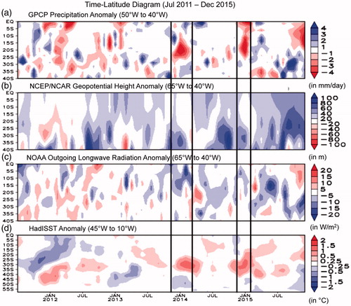
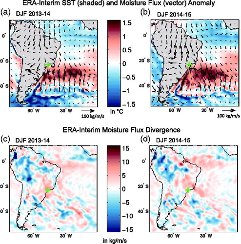
To investigate the contributions of large scale circulation changes to the precipitation deficit over state of São Paulo, we compare time-lags between precipitation anomalies and anomalies in SST, geopotential height at 200 hPa from NCEP/NCAR (Kalnay et al., 1996) and outgoing longwave radiation (OLR) from NOAA (Liebmann and Smith 1996) for the period 2011 till 2015, including the manifestation and/or absence of SACZ (Fig. 3a–d). This analysis indicates that geopotential height anomalies, located to the south of São Paulo (Fig. 3b), precede the precipitation anomalies in 2013/14 and 2014/15. SST anomalies (Fig. 3d) are time-synchronous (contemporaneous) with the precipitation anomalies and OLR anomalies occurring similarly at the same time as precipitation anomalies, as expected (Fig. 3c).

Fig. 3. Time latitude diagram of meridionally averaged (a) precipitation anomaly (GPCP), (b) Geopotential height anomaly (NCEP/NCAR), (c) Outgoing longwave radiation anomaly (NOAA) and (d) SST anomaly for the period July 2011 to December 2015. The precipitation has been averaged over São Paulo, i.e. 50°W to 40°W, whereas the other three variables have been averaged over the south Atlantic Ocean. Geopotential height and OLR have been averaged over 65°W to 40°W and SST has been averaged over 45°W to 10°W. The monthly anomalies of the climatic fields have been calculated with respect to the mean of the respective months during the whole period i.e. 1979–2004.

The large-scale spatial patterns of rainfall and SST anomalies for the peak rainy season (DJF) between 2013 and 2015 are shown in Fig. 4a–f based on the GPCP climatology and ERA-Interim reanalysis and with reference to the 1979–2004 period. Large-scale patterns of rainfall are quite similar in both 2013/14 and 2014/15 (Fig. 4a and b) with both years showing a negative precipitation anomaly over southeastern Brazil, which includes São Paulo (green cross). The negative precipitation anomaly extends in a southeastward direction into the subtropical South Atlantic in both years. In these 2 years, the negative anomaly over São Paulo is also associated with positive rainfall anomalies to the south of São Paulo, in the La Plata basin, SESA (Southeast South Asia) and over the western part of the Amazon basin. The dipole pattern observed in these 2 years agrees well with other studies (Espinoza et al., 2014; Coelho et al., 2016b; Cavalcanti et al., 2017). In 2015/16 São Paulo, received normal amounts of rainfall consistent with Zhang et al. (2016), while a negative precipitation anomaly of about 2–3 mm/day can be observed towards the eastern part of Amazon basin. At a larger scale, the precipitation anomaly pattern has a dipole-like structure over Brazil (Fig. 4c) consistent with El Niño conditions; the southern part of Brazil shows excessive rainfall whereas the northern part shows a rainfall deficit.

Fig. 4. December to February (DJF) rainfall anomaly (in mm/day) and SST (in °C) for 2013/14, 2014/15 and 2015/16. The rainfall has been adopted from GPCP (Adler et al., 2003) and the SST is from ERA-Interim (Dee et al., 2011). The top panel (a–c) shows the rainfall anomalies while the bottom panel (d–f) shows the SST anomalies. The geographical location of São Paulo city has been marked as green plus sign in all the subplots. We have chosen a box over the South Atlantic Ocean, which has been used to identify the similar occurrence of SST anomaly pattern in the future climate.

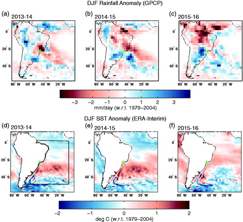
Figure 4d and e show the observed SST anomaly from ERA-Interim in DJF 2013/14 and 2014/15, respectively. The anomalies are very similar suggesting a possible association between these SST anomalies and the observed precipitation deficit over São Paulo 2 years in a row. The SST anomalies consist of three zonal bands: a cold band in the tropical Atlantic (10°N to 20°S), a warm band just to the south of São Paulo (20°S to 40°S, roughly the oceanic part of the SACZ region), and another cold band poleward of 40°S. In both rainfall-deficit years, warm anomalies were also observed over the Indonesian Pacific and cold anomalies over equatorial central Pacific (see Supplementary Fig. S3a, b), which is consistent with Seth et al. (2015) and Coelho et al. (2016b). Usually, the subtropical high over the South Atlantic forms far from the South American coast with core towards the eastern part of the South Atlantic. But in 2013/14, this high-pressure system has formed much closer to the coast extending towards northeast Brazil, resulting in the absence of the formation of SACZ episodes in 2013/14 (Coelho et al., 2016b; Nobre et al., 2016). These analyses largely agree with the inferences made by Otto et al. (2015), Seth et al. (2015) and the analysis performed by Coelho et al., (2016a, 2016b). The warm SST band near São Paulo seen in 2013–2015 shifted northward in 2015/16 (Fig. 4f) resulting in positive rainfall anomalies west of São Paulo (Fig. 4c). The mechanism behind the absence of SACZ was the prolonged atmospheric blocking near Sao Paulo (Coelho et al., 2016b).

3.1.3 Vertically integrated moisture flux transports and divergence

Moisture flux transport relates to precipitation, thus insights on drought mechanisms can be gained by analyzing moisture flux transport and its divergence (with positive divergence indicative of absence of precipitation). During the two rainfall-deficit years the column-integrated moisture flux advected into the São Paulo region was mostly from the North (Fig. 5a and b). In these years, there was a strong divergence observed over São Paulo (Fig. 5c and d), which is consistent with the occurrence of negative precipitation anomalies. In contrast, there is a strong convergence zone over the western Amazon and a weak divergence over the La Plata basin in both the deficit years, which is associated with excessive rainfall over the corresponding regions (Fig. 5c and d).

Fig. 5. Top panel: Moisture flux transport anomaly and SST anomaly (°C) obtained from ERA-Interim for (a) 2013/14 and (b) 2014/15 with respect to the mean of the respective fields during 1979–2004. The moisture flux transport has been plotted as vector field while the SST anomaly has been plotted as shaded. Bottom panel: moisture flux anomaly divergence for (c) 2013/14 and (d) 2014/15.

3.2 Model-based examination of the role of Amazon deforestation and GHG emissions on the São Paulo water shortage

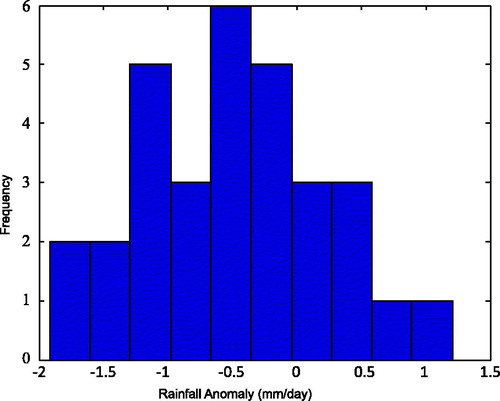
To investigate the roles of deforestation in the Amazon and changes in the climate system caused by increases in GHGs for the anomalously low rainfall event in 2013/14, we carried out three simulation scenarios with HadAM3 as described in Section 2 and summarized in Table 1. Comparing different ensemble members, we find that there is a precipitation deficit during 2013/14 in the São Paulo region (defined as above) in four out of six, and five out of six of the simulations for scenarios 1 and 2, respectively. For the 31 ensemble simulations for scenario 3, 74% of the simulations showed a precipitation deficit (see Fig. 6), suggesting that SST’s anomaly patterns as in 2013/14 are associated with drier than usual conditions in the São Paulo region, although reflecting the chaotic nature of atmospheric circulation this is not always the case, i.e. there seem to be at least two possible modes. To identify and display the spatial patterns associated with the dry mode in the results that follow we only averaged the negative rainfall members.

Fig. 6. Frequency distribution of DJF 2013/14 rainfall anomaly over the São Paulo region (25^oS to 20^oS and 50^oW to 45^oW) from HadCM3 simulations with observed land cover and observed GHG. Total 31 numbers of ensemble simulations were carried out by perturbing the initial conditions.

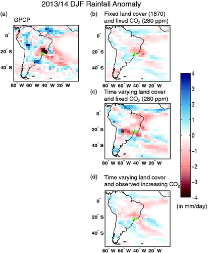
We first compare the simulated rainfall anomalies in DJF 2013/14 with respect to 1979–2004 mean rainfall as documented by gridded observed rainfall from GPCP (Fig. 7). Large-scale simulated precipitation patterns are broadly similar between the different simulation scenarios, all showing on average a negative precipitation anomaly over southeastern Brazil, including the São Paulo region, although the anomalous pattern is slightly displaced northwards when compared to the observed pattern. In both GPCP observations (Fig. 7a) and model simulations (Fig. 7b–d) the precipitation anomaly extends in the southeastward direction into the subtropical South Atlantic. All simulations capture not only the São Paulo region anomaly but also the excess rainfall pattern over the western part of the Amazon basin. However, the rainfall anomaly patterns in the two simulations with vegetation changing over time including recent deforestation over Amazon forest (Fig. 7c and d) are slightly closer to GPCP precipitation anomalies (Fig. 7a) compared to the simulation with fixed vegetation (Fig. 7b). Thus, according to these simulations, even in the presence of unperturbed forests (Fig. 7b), the low precipitation anomaly over São Paulo is reproduced by the model. With the caveat that observed SSTs may already be influenced by deforestation of the Amazon, our simulations thus suggest that the São Paulo precipitation deficit is indeed related primarily to the specific SST anomalies in these years with deforestation/vegetation cover change or the direct effect of increasing GHG levels slightly modulating the anomalies. We also make the caveat that we cannot discern to what extent the positive SST anomalies are enhanced by lack of clouds impeding solar radiation.

Fig. 7. DJF rainfall anomaly (mm/day) for 2013/14 (right panel) with respect to 1979–2004 from observations and HadAM3 simulations. Left and right columns represent observed and model simulated rainfall anomaly for 2013/14 respectively. (a) Observed rainfall from GPCP rainfall, b) simulation result of HadAM3 with fixed land cover (1870) and CO₂ fixed at preindustrial level (Scenario 1), (c) simulation results using HadAM3 with reconstructed time varying land cover (Meiyappan and Jain, 2012) and CO₂ fixed at preindustrial level (Scenario 2) and (d) simulation results using HadAM3 with reconstructed time varying land cover (Meiyappan and Jain, 2012) and observed GHGs increasing over time (Scenario 3). In this figure, the selection of the ensembles is based on criteria when the ensemble member simulates the rainfall anomaly over the São Paulo region (25^oS to 20^oS and 50^oW to 45^oW) less than –1 mm/day. Then the composite of these ensembles have been calculated and plotted above.

3.3 Past and future frequency of dry events like 2013/14 in the São Paulo region

How unique are the SST conditions experienced during the wet season of 2013/14? In order to obtain at least a tentative answer for this question both for the historical record and future climate simulations, we apply a simple pattern recognition approach (Santer et al., 1995) both to the historical record and future climate simulations. The pattern recognition approach calculates for each year a correlation coefficient (CC) of spatial patterns of SST anomalies in the South Atlantic (region shown in Fig. 4d), with the spatial pattern of the anomaly in DJF 2013/14. High positive correlation values indicate a similar (spatial) SST condition to 2013/14. To calculate the correlation coefficients, spatial patterns are arranged as vectors and then the correlation coefficient calculated in the standard way. For example, if the spatial map consists of N x M pixels, then these are arranged as a vector $\overrightarrow{s}=\left(s_{1,1,\dots ,}{s}_{2,1,\dots ,}{s}_{2,N,\dots },s_{M,1,\dots }{s}_{M,\dots ,N}\right)$ where $s_{1,1\dots ,}{s}_{1,N,}$ is the first column of pixels of the map and so on.

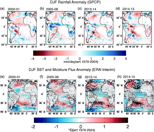
We first test the approach by applying it to the ERA-Interim SST anomaly over the region in the Atlantic marked in Fig. 4d for the 1979–2015 period (Fig. 8). There are 3 years when correlation values exceed the 90th percentile of the time series (Fig. 8), viz. 2000–01 (CC value 0.76), 2005–06 (CC value 0.72) and 2014/15 (CC value 0.85), and the four events for which patterns are most anti correlated (below the 10th percentile): 1984–85 (CC value –0.74), 1999–00 (CC value –0.54), 2004–05 (CC value –0.51) and 2008–09 (CC value –0.4). The frequency distribution of pattern correlation coefficients of SST anomaly over tropical South Atlantic Ocean for the period 1979–2015 is provided in Fig. 8b. Events with high positive correlation occurred three times over this 36-year period. The spatial map of rainfall and SST anomalies for the years having highest correlation values (greater than 90th percentile) are plotted in Fig. 9, whereas similar plots for the most anti-correlated years (less than 10th percentile) have been provided in Supplementary Fig. S5. In 2000–01, 2005–06 and 2014/15, the spatial patterns of the rainfall, SST and moisture flux anomaly near São Paulo were indeed similar to that in the 2013/14 (Fig. 9). In the anti-correlated years 1984–85, 1999–00, 2004–05 and 2008–09 there were positive rainfall anomalies over the São Paulo region (Supplementary Fig. S5). Also, we analysed the duration of the surface pressure anomaly associated with blocking during the highest and lowest correlated years over the Sao Paulo region (Supplementary Fig. S4). The durations of the pressure anomaly for the years with similar anomalies are similar to the duration in 2013/14.

Fig. 8. (a) Pattern correlation of SST anomaly from ERA-Interim of DJF 2013/14 over south Atlantic (region shown in Fig. 3d i.e. 60°S to 0 and 42°W to 10°W) with SST anomaly in the other years. Red lines denote the years when the correlation is greater than or equal to 90th percentile and blue lines denote the years when the correlation is less than or equal to 10th percentile. (b) Frequency distribution of pattern correlation coefficients of ERA-Interim SST anomalies for 1979–2015.

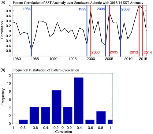
Fig. 9. DJF rainfall anomaly (GPCP), SST and moisture flux transport anomaly (ERA-Interim) during the years having correlation value greater than or equal to 90th percentile (Fig. 8) of the study period viz. 2000–01, 2005–05, 2013–14 and 2014–15. Top panel: rainfall anomaly for the years 2000–01 (a), 2005–06 (b), 2013–14 (c) and 2014–15 (d). Bottom panel: SST (in shaded) and moisture flux transport (in vector) anomaly for the years 2000–01 (e), 2005–06 (f), 2013–14 (g) and 2014–15 (h).

We further apply the pattern recognition approach to historical and future climate simulations with three well-known CMIP5 models: CCSM4, GFDL-ESM2M and HadGEM2-ES for the historical period (1860–2005) and future period (2006–2100) based on the RCP 8.5 emissions scenario (Collins et al., 2011). The choice of the CMIP5 models has been made based on its ability to reproduce the precipitation and OLR pattern in the SACZ and SESA region (Junquas et al., 2012). This has been performed by calculating the climatological DJF mean of precipitation and OLR for the period 1979–2005 for selected three models (viz. CCSM4, GFDL-ESM2M and HadGEM2-ES) and corresponding observations. Precipitations from GPCP and OLR from NOAA have been used as observations for validating the CMIP5 models. The CMIP5 models have performed satisfactorily in reproducing the precipitation (see Supplementary Fig. S6) and OLR pattern over SACZ and SESA region (see Supplementary Fig. S7). Further, the precipitation changes in the future period (2050–2075) with respect to the historical period (1979–2004) suggest that the seesaw pattern exists (see Supplementary Fig. S8), which is consistent with Junquas et al. (2012). It is interesting to note that, on average, rainfall in São Paulo region is higher in the future (see Supplementary Fig. S8).

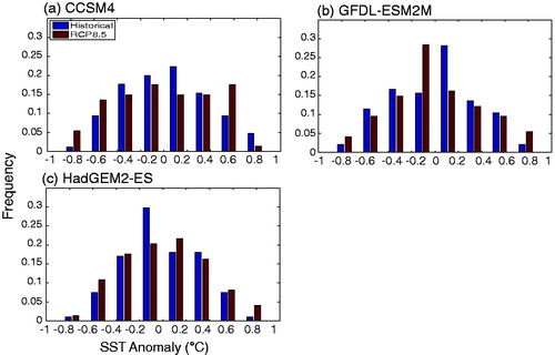
The spatial correlation was calculated between the SST anomalies of 2013/14 from ERA-Interim with each year’s SST anomaly from the selected three CMIP5 models over the tropical South Atlantic Ocean (Fig. 10a–c). We use a moving window of 20 years to calculate SST anomalies to take into account the temperature increases of the ocean in these simulations. Also, the rainfall anomaly over São Paulo has been plotted for the historical and future periods for the same models (Fig. 10d–f). The analysis shows that for years in which historical SST correlations over the tropical South Atlantic Ocean are higher than 90th percentile of the corresponding rainfall anomalies over São Paulo were indeed negative in 67% of the cases in CCSM4 and in around 90% of cases in GFDL-ESM2M and HadGEM2-ES, thus confirming the consistency of the approach. The normalized frequency distributions of the correlation coefficients of three CMIP5 models for the past and future shows that there is no clear indication of an increase of 2013/14 SST anomaly events in any of the model predictions of future climate (Fig. 11a–d).

Fig. 10. Left panel represents the pattern correlation coefficients of SST anomaly of DJF 2013/14 from ERA-Interim with SST anomaly of other years for simulations with CCSM4 (a), GFDL-ESM2M (b) and HadGEM2-ES (c) for the period 1870–2100. Right panel represents the rainfall anomaly over the São Paulo region (25^oS to 20^oS and 50^oW to 45^oW) from CCSM4 (d), GFDL-ESM2M (e) and HadGEM2-ES (f) for the period 1870–2100. The blue and red curves represent historical and future periods in RCP8.5 scenario respectively. Black vertical lines in Fig. 8a–c indicate the years when the correlation value is more than 90th percentile and in Fig. 8d–f, the black vertical line shows the rainfall anomalies for the corresponding years.

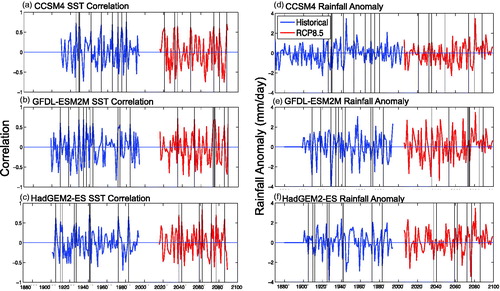
Fig. 11. Frequency distribution (normalized by division by total number of years) of pattern correlation coefficients (shown in Fig. 10) of SST anomalies for the simulations with CCSM4 (a), GFDL-ESM2M (b) and HadGEM2-ES (c) for the period 1870–2100. The blue and red bars represent historical and future periods in RCP8.5 scenario respectively.

4. Conclusions

Building on previous studies, we have further investigated the factors contributing to the recent water shortage over São Paulo over the period 2013/14 and 2014/15, using a combination of observations, reanalysis datasets and model simulations. We have specifically analysed the role of deforestation and elevated GHG levels for the 2013/14 and 2014/15 anomalies using a set of factorial coupled land-vegetation-atmosphere ensemble simulations, driven by observed SSTs. From the simulation results we conclude that an anomalous high pressure system was established over anomalously warm SSTs in the southern Atlantic Ocean, with the warm ocean maintained by prevailing subsidence and enhanced solar radiation reaching the surface. These factors were found to be directly associated with the precipitation deficit, while deforestation and increasing GHGs only slightly modified the character of the precipitation anomalies. The results of the time-varying GHG experiment presented in the manuscript agree with experiments by Otto et al. (2015) with respect to unchanged precipitation response when comparing the current with pre-industrial GHG conditions. Historical records and a pattern recognition analysis suggest further that spatiotemporal SST and precipitation anomalies similar to those in 2013/14 have occurred three times over the last 35 years. Finally, the analysis of future climate simulations from three different CMIP5 models does suggest that similar SST anomalies in the southern Atlantic and associated events of precipitation deficit are likely to occur with similar frequency in the future. These results need to be taken with sufficient caution given limitations of climate models and of our approach.

Supplemental material

Supplemental material for this article can be accessed here: https://doi.org/10.1080/16000870.2018.1481690.

Acknowledgements

We are thankful to the Brazilian National Meteorological Service (INMET), water and waste management company of São Paulo (SABESP), the University of São Paulo (USP), GPCP and ECMWF for making their data records available for this study. We acknowledge the support from the NERC (UK Natural Environment Research Council) AMAZONICA and Amazon Hydrological Cycle grants (NE/F005806/1 and NE/K01353X/1) and the SPECS project (Grant Agreement No. 308378) funded by the European Commission’s Seventh Framework Research Programme. CASC was supported by Conselho Nacional de Desenvolvimento Científico e Tecnológico (CNPq) processes 304586/2016-1. We also acknowledge the support provided by Fundação de Amparo à Pesquisa do Estado de São Paulo (FAPESP) Processes 2015/50687-8 (CLIMAX Project). JB acknowledges support from CONICYT/FONDAP/1511000. The Historical Land-Cover Change and Land-Use Conversions Global Dataset used in this study were acquired from NOAA’s National Climatic Data Center (http://www.ncdc.noaa.gov/). BBLC acknowledges the support from CNPq Science Without Borders (207400/2014-8).

Disclosure statement

No potential conflict of interest was reported by the authors.

References

- Adler, R. F., Huffman, G. J., Chang, A., Ferraro, R., Xie, P.-P. and co-authors. 2003. The version 2 global precipitation climatology project (GPCP) monthly precipitation analysis (1979–Present). J. Hydrometeor. 4, 1147–1167. DOI:10.1175/1525-7541(2003)004<1147:TVGPCP>2.0.CO;2.
- Barros, V. R., González, M., Liebmann, B. and Camilloni, I. 2000. Influence of the South Atlantic convergence zone and South Atlantic sea surface temperature on the interannual summer rainfall variability in southern South America. Theor. Appl. Climatol. 67, 123–183. DOI:10.1007/s007040070002.
- Cabré, M. F., Solman, S. and Núñez, M. 2016. Regional climate change scenarios over southern South America for future climate (2080–2099) using the MM5 Model. Mean, interannual variability and uncertainties. ATM 29, 35–60. DOI:10.20937/ATM.2016.29.01.04.
- Carvalho, L. M. V., Jones, C. and Liebmann, B. 2004. The South Atlantic convergence zone: intensity, form, persistence, and relationships with intraseasonal to interannual activity and extreme rainfall. J. Climate 17, 88–108. DOI:10.1175/1520-0442(2004)017<0088:TSACZI>2.0.CO;2.
- Cavalcanti, I. F. A., Marengo, J. A., Alves, L. M. and Costa, D. F. 2017. On the opposite relation between extreme precipitation over west Amazon and southeastern Brazil: Observations and model simulations. Int. J. Climatol. 37, 3606–3618. DOI:10.1002/joc.4942.
- Chou, S. C., Marengo, J. A., Lyra, A. A., Sueiro, G., Pesquero, J. F. and co-authors. 2012. Downscaling of South America present climate driven by 4-member HadCM3 runs. Clim. Dyn. 38, 635. DOI:10.1007/s00382-011-1002-8.
- Coelho, C. A. S., Cardoso, D. H. F. and Firpo, M. A. F. 2016a. Precipitation diagnostics of an exceptionally dry event in São Paulo, Brazil. Theor. Appl. Climatol. 125, 769–784. DOI:10.1007/s00704-015-1540-9.
- Coelho, C. A. S., de Oliveira, C. P., Ambrizzi, T., Reboita, M. S., Carpenedo, C. B. and co-authors. 2016b. The 2014 southeast Brazil austral summer drought: regional scale mechanisms and teleconnections. Clim. Dyn. 46, 3737–3752. DOI:10.1007/s00382-015-2800-1.
- Collins, W. J., Bellouin, N., Doutriaux-Boucher, M., Gedney, N., Halloran, P. and co-authors. 2011. Development and evaluation of an earth system model HadGEM2. Geosci. Model Dev. 4, 1051–1062. DOI:10.5194/gmd-4-1051-2011.
- Coutinho, R. M., Kraenkel, R. A. and Prado, P. I. 2015. Catastrophic regime shift in water reservoirs and São Paulo water supply crisis. PLoS ONE 10, e0138278. DOI:10.1371/journal.pone.0138278.
- Dee, D. P., Uppala, S. M., Simmons, A. J., Berrisford, P., Poli, P. and co-authors. 2011. The ERA-Interim reanalysis: configuration and performance of the data assimilation system. Quar. J. Royal. Meteorol. Soc. 137, 553–597. DOI:10.1002/qj.828.
- Dunne, J. P., John, J. G., Adcroft, A. J., Griffies, S. M., Hallberg, R. W. and co-authors. 2012. GFDL’s ESM2 global coupled climate–carbon earth system models. Part I: physical formulation and baseline simulation characteristics. J. Climate 25, 6646–6665. DOI:10.1175/JCLI-D-11-00560.1.
- Dunne, J. P., John, J. G., Shevliakova, E., Stouffer, R. J., Krasting, J. P. and co-authors. 2013. GFDL’s ESM2 global coupled climate–carbon earth system models. Part II: carbon system formulation and baseline simulation characteristics. J. Climate 26, 2247–2267. DOI:10.1175/JCLI-D-12-00150.1.
- Escobar, H. 2015. Drought triggers alarms in Brazil’s biggest metropolis. Science 347, 812. DOI:10.1126/science.347.6224.812.
- Espinoza, J. C., Marengo, J. A., Ronchail, J., Carpio, J. M., Flores, L. N. and co-authors. 2014. The extreme 2014 flood in south-western Amazon basin: the role of tropical–subtropical South Atlantic SST gradient. Environ. Res. Lett. 9, 124007. DOI:10.1088/1748-9326/9/12/124007.
- Gent, P. R., Danabasoglu, G., Donner, L. J., Holland, M. M., Hunke, E. C. and co-authors. 2011. The community climate system model version 4. J. Climate 24, 4973–4991. DOI:10.1175/2011JCLI4083.1.
- Getirana, A. 2016. Extreme water deficit in Brazil detected from space. J. Hydrometeor. 17, 591–599. DOI:10.1175/JHM-D-15-0096.1.
- Herdies, D. L., DaSilva, A., Silva Dias, M. A. F. and Ferreira, R. N. 2002. The moisture budget of the bimodal pattern of the summer circulation over South America. J. Geophys. Res. 107, 8075.
- Junquas, C., Vera, C., Li, L. and Le Treut, H. 2012. Summer precipitation variability over southeastern South America in a global warming scenario. Clim. Dyn. 38, 1867–1883. DOI:10.1007/s00382-011-1141-y.
- Kalnay, E., Kanamitsu, M., Kistler, R., Collins, W., Deaven, D. and co-authors. 1996. The NMC/NCAR 40-year reanalysis project. Bull. Am. Meteor. Soc. 77, 437–471. DOI:10.1175/1520-0477(1996)077<0437:TNYRP>2.0.CO;2.
- King, D., Schrag, D., Zhou, D., Ye, Q. and Ghosh, A. 2015. Climate change: a risk assessment—risk assessment part 3: systemic risks. In: Centre for Social Science and Policy (eds. J. Hynard and T. Rodger), London, pp. 110–111.
- Kodama, Y. M. 1993. Large-scale common features of sub-tropical precipitation zones (the Baiu Frontal Zone, the SPCZ, and the SACZ). Part I: characteristics of subtropical frontal zones. J. Meteorol. Soc. Jpn. 71, 581–835. DOI:10.2151/jmsj1965.71.5_581.
- Kolusu, S. R., Marsham, J. H., Mulcahy, J., Johnson, B., Dunning, C., and co-authors. 2015. Impacts of Amazonia biomass burning aerosols assessed from short-range weather forecasts. Atmos. Chem. Phys. 15, 12251–12266. DOI:10.5194/acp-15-12251-2015.
- Liebmann, B. and Smith, C. A. 1996. Description of a complete (Interpolated) outgoing longwave radiation dataset. Bull. Am. Meteorol. Soc. 77, 1275–1277.
- Marengo, J. A. and Alves, L. M. 2015. Crise hídrica em São Paulo em 2014: seca e desmatamento [Water crisis in São Paulo in 2014: drought and deforestation]. GEOUSP, USP- São Paulo.
- Meiyappan, P. and Jain, A. K. 2012. Three distinct global estimates of historical land-cover change and land-use conversions for over 200 years. Front. Earth Sci. 6, 122–139. DOI:10.1007/s11707-012-0314-2.
- Munich, R. 2015. Natural catastrophes 2014. analyses, assessments, positions. TOPICS-GEO 2014, Munich, 67 p.
- Nazareno, A. G. and Laurance, W. F. 2015. Brazil’s drought: beware deforestation. Science 347, 1427. DOI:10.1126/science.347.6229.1427-a.
- Nobre, C. A., Marengo, J. A., Seluchi, M. E., Cuartas, L. A. and Alves, L. M. 2016. Some characteristics and impacts of the drought and water crisis in Southeastern Brazil during 2014 and 2015. J. Water Res. Protect. 8, 2.
- Otto, F. E. L., Coelho, C. A. S., King, A., De Perez, E. C., Wada, Y. and co-authors. 2015. Factors other than climate change, main drivers of 2014/15 water shortage in Southeast Brazil [in “Explaining extremes of 2014 from a climate perspective”]. Bull. Am. Meteor. Soc. 96, S35–S40. DOI:10.1175/BAMS-D-15-00120.1.
- Peterson, T. C. and Vose, R. S. 1997. An overview of the global Historical Climatology Network temperature database. Bull. Am. Meteor. Soc. 78, 2837–2849.
- Pope, V., GallanI, M., Rowntree, P. and Stratton, R. 2000. The impact of new physical parametrizations in the Hadley Centre climate model: HadAM3. Clim. Dyn. 16, 123–146. DOI:10.1007/s003820050009.
- Rayner, N. A., Parker, D. E., Horton, E. B., Folland, C. K., Alexander, L. V., and co-authors. 2003. Global analyses of sea surface temperature, sea ice, and night marine air temperature since the late nineteenth century. J. Geophys. Res. 108, 4407.
- Reboita, M. S., da Rocha, R. P., Dias, C. G. and Ynoue, R. Y. 2014. Climate projections for South America: RegCM3 driven by HadCM3 and ECHAM5. Adv. Meteorol. 2014, 1. DOI:10.1155/2014/376738.
- SABESP – COMPANHIA DE SANEAMENTO BÁSICO DO ESTADO DE SÃO PAULO. 2008. Dossiê – Sistema Guarapiranga. São Paulo: Sabesp, setembro de. 16 p. Online at: http://memoriasabesp.sabesp.com.br/acervos/dossies/pdf/9_sistema_guarapiranga.pdf
- Santer, B. D., Taylor, K. E., Wigley, T. M. L., Penner, J. E., Jones, P. D. and Cubasch, U. 1995. Towards the detection and attribution of an anthropogenic effect on climate. Clim. Dyn. 12, 77–100. DOI:10.1007/BF00223722.
- Seth, A., Fernandes, K. and Camargo, S. J. 2015. Two summers of São Paulo drought: origins in the western tropical Pacific. Geophys. Res. Lett. 42, 816–823.
- Shepherd, J. M., Pierce, H. and Negri, A. J. 2002. Rainfall modification by major urban areas: Observations from spaceborne rain radar on the TRMM satellite. J. Appl. Meteorol. 41, 689–701. DOI:10.1175/1520-0450(2002)041<0689:RMBMUA>2.0.CO;2.
- Silva, W. L., Nascimento, M. A. and Menezes, W. F. 2015. Atmospheric blocking in the South Atlantic during the summer 2014: a synoptic analysis of the phenomenon. ACS. 5, 386–393. DOI:10.4236/acs.2015.54030.
- Swiss-Re. 2015. Natural catástrofes and man-made disasters in 2014: convective and winter storms generate most losses. Swiss Re Ltd-Economic Research and Consulting, Zurich, Swiss Re-Sigma No. 2/2015, 52 p.
- Taylor, K. E., Stouffer, R. J. and Meehl, G. A. 2012. An overview of CMIP5 and the experiment design. Bull. Am. Meteorol. Soc. 93, 485–498. DOI:10.1175/BAMS-D-11-00094.1.
- UNICA 2015. Centre for Food Storage and Market Distribution of the State of São Paulo (CEAGESP), the Brazilian Citrus Association, the Cereal Stock Market of São Paulo and the Brazilian Union of Sugar Cane Producers. Online at: http://www.unica.com.br/
- United Nations, Department of Economic and Social Affairs, Population Division. 2015. World Urbanization Prospects: The 2014 Revision, (ST/ESA/SER.A/366).
- Zhang, H., Delworth, T., Zeng, F., Vecchi, G., Paffendorf, K. and Jia, L. 2016. Detection, attribution, and projection of regional rainfall changes on (multi-) decadal time scales: a focus on southeastern South America. J. Climate 29, 8515–8534. DOI:10.1175/JCLI-D-16-0287.1.