On the structure and stability of the hurricane eyewall

Abstract

This study examines the structure and related stability of the hurricane eyewall at the mature stage. By treating the hurricane eyewall as a rotating fluid annulus, it is shown that axisymmetric steady-state solutions for the hurricane wind field can be explicitly obtained in the eyewall region. Using the energy method, we show that this class of the steady-state solutions is nonlinearly stable, thus explaining the resilience of the hurricane eyewall structure and intensity at the mature stage as established from previous observational and modelling studies.

Keywords:

• vortex dynamics
• stability analysis
• energy method
• hurricane intensity equilibrium
• tropical cyclones

1. Introduction

Hurricanes are essentially dynamical systems that are driven by energy transfer from the warm ocean surface. A typical development of a hurricane consists of several stages including an early tropical disturbance, a tropical depression, a tropical storm and finally a hurricane stage. Among these four stages of development, the mature stage with a distinct cloud-free eye area wrapped around by an annulus wall of cloud, the so-called hurricane eyewall, plays an important role in understanding the large-scale controls of ambient environment on hurricane intensity variation (e.g. Black and Willoughby, 1992; McNoldy, 2004; Marks et al., 2008; Sitkowski et al., 2011; Zhou et al., 2011; Hazelton et al., 2015). Due to the complexity of hurricane physics and dynamic-thermodynamic feedbacks, an exact solution for the hurricane overall structure as well as the related eyewall at the mature stage has not been fully known. Most often, the hurricane inner-core structure is either derived from a simplified balanced dynamics or indirectly inferred from numerical simulations.

The early works by Depperman (1947), Malkus and Riehl (1960) and Riehl (1963) appeared to be among the first that shed some light on a diagnostic relationship between the wind and thermal structures in the inner-core region. By assuming an empirical relation for the surface eddy stress, Riehl (1963) found a specific radial distribution of the azimuthal wind in the planetary boundary layer (PBL) and another relationship for the outflow layer. Likewise, Malkus and Riehl (1960) obtained a similar radial profile for the azimuthal wind in the PBL under an assumption of a well-mixed boundary and a constant surface drag coefficient. Among several hurricane wind profiles examined in these early studies, the Rankine vortex structure and its variations have emerged as the most plausible approximation for the hurricane wind at the mature stage. This is because the hurricane inner core highly resembles a rotating solid body, and the Rankine profile derived from the solid-body rotation is therefore plausibly applicable for the hurricane central region (see, e.g. Kelvin, 1880; Depperman, 1947; Riehl, 1963; Malkus and Riehl, 1960; Carrier et al., 1971; Anthes, 1974; Holland, 1980). Although this Rankine structure contains the radius of maximum wind (RMW) similar to that in the eyewall of a real hurricane, its sharp separation of the azimuthal wind field between the inner core and outer core regions at the RMW location is too idealized and does not allow for realistic eyewall structure.

From a broader context of general fluid systems, a number of other two-dimensional (2D) steady-state structure for axisymmetric vortices beyond the Rankine profile have been also obtained under different simplifications such as in the absence of the surface drag or incompressible inviscid fluid. For example, several classes of steady-state solutions have been found in previous theoretical studies including the Burgers vortex (Wang, 1991), the Sullivan vortex (Wu et al., 2006) or a family of general sink vortices (Sun, 2011), which are basically solutions for incompressible inviscid flows. Although these exact solutions share some similarity to the hurricane wind distribution, there are a number of subtle characteristics of the hurricane eyewall that those solutions do not possess such as the strong vertical motion in the narrow eyewall region but negligible outside the eyewall, or the dominance of the cyclonic wind throughout the troposphere in the inner-core region. These subtle structures of the hurricane eyewall explain why the aforementioned exact solutions are not entirely applicable for the eyewall of mature hurricanes.

From the physical perspective, the particular concerns about the hurricane eyewall emerge not only because of the unique characteristics of the hurricane eyewall dynamics, but also because this is the area where the peak intensity of hurricanes, which is typically represented by the maximum sustainable wind speed at 10-m altitude, occurs. Using the gradient wind balance under the neutral slantwise convection condition, Emanuel (1986) showed that the maximum potential intensity (MPI) limit that a hurricane can reach in the axisymmetric framework is given by an explicit function of sea surface temperature, outflow temperature and disequilibrium of enthalpy at the ocean surface. Subsequent extension of Emanuel’s MPI framework led to a number of additional analytical and numerical studies on this hurricane steady-state limit that were supported by various numerical simulations (see, e.g. Emanuel, 1988, 1995; Bryan and Rotunno, 2009; Hakim, 2011; Wirth and Dunkerton, 2006). While this steady-state solution is of importance to current studies of hurricane intensity, Emanuel’s MPI limit is nevertheless a point-like value that represents the maximum surface wind at the RMW location only. Hence, there is no explicit radial or vertical structure of the hurricane wind distribution inside the eyewall region in this MPI framework.

For practical applications, it should be emphasized that finding a steady-state solution for a dynamical system is just one aspect of the problem. Another equally important question is whether this solution is stable or not. That is, a steady-state solution is considered a physical solution only if it is at least locally stable. Otherwise, any small perturbation would quickly destroy the steady state. In an attempt to address the stability of Emanuel’s steady-state MPI limit, Schonemann and Frisius (2012), Kieu (2015) and Kieu and Wang (2017a, 2017b) presented a simple low-order model based on the fundamental scales of hurricane characteristics. Their detailed stability analyses revealed that hurricanes indeed possess an MPI equilibrium that is asymptotically stable. The structurally stable property of the MPI equilibrium is held for a wide range of model parameters, regardless of model initial conditions or numerical configurations. Due to the point-like nature of these low-order hurricane models, the proof of the MPI stability in these stability analyses is again valid only for a single value rather than for the entire hurricane eyewall structure.

Given various modelling and observational studies that consistently display a similar hurricane steady state with a coherent eyewall structure in favourable environmental conditions, it is desirable from the theoretical perspective to examine if hurricane dynamics leads to a preferred eyewall structure, and if so, how this eyewall structure can be maintained with time. With these questions, the main objectives of this study are to (1) seek a steady-state solution that can plausibly represent the hurricane eyewall structure above the PBL at the mature stage, and (2) quantify the stability of this steady-state solution to ensure that the eyewall solution is physically realizable.

The rest of this paper is thus organized as follows. Section 2 presents a set of governing equations for hurricane dynamics and derivations of the steady-state solution for the hurricane eyewall along with a proof of the stability for this solution. Discussions about the limitations of our steady-state solution and related assumptions are provided in Section 3, and concluding remarks are summarized in Section 4.

2. Hurricane dynamics

2.1. Governing equations

Because of the compressible nature of hurricane dynamics, we consider in this study a common model for hurricanes that is based on the anelastic approximation in the isobaric coordinate as follows (e.g. Miller, 1974; Miller and White, 1984; Haltiner and Williams, 1980; Holton, 2004):(1) $$\frac{\partial {\mathbf{V}}_{\mathrm{h}}}{\partial t}+(\mathbf{v}·\nabla ){\mathbf{V}}_{\mathrm{h}}=-{\nabla }_{\mathrm{h}}\varphi -f\mathbf{k}\times {\mathbf{V}}_{\mathrm{h}}+{\mathbf{F}}_{\mathrm{h}},$$(1) (2) $$\frac{\partial w}{\partial t}+(\mathbf{v}·\nabla )w=-\overline{\rho }\left(p\right)g\frac{\partial \varphi }{\partial p}+\frac{g(T-\overline{T})}{\overline{T}}\mathbf{k}+F_{\mathrm{w}},$$(2) (3) $$\frac{\partial T}{\partial t}+({\mathbf{V}}_{\mathbf{h}}·\nabla )T+S\omega =Q,$$(3) (4) $$\nabla ·\mathbf{v}=0,$$(4) where $\omega \equiv \mathrm{d}p/\mathrm{d}t$ is the vertical motion in the isobaric coordinate, ${\mathbf{V}}_{\mathrm{h}}\equiv (u,v)$ is the horizontal velocity field, f is the Coriolis parameter, T is the temperature, Q is net heating per unit mass, ρ is the atmospheric density, k is the unit vector in the vertical direction, $\varphi \equiv gz$ is the geopotential perturbation relative to the hydrostatic reference state based on the reference density $\overline{\rho }(p)$ and $\overline{T},{\nabla }_{\mathrm{h}}$ is the gradient operator in the horizontal directions, $S\equiv \frac{(g/C_{\mathrm{p}}-\partial T/\partial z)}{\rho g}$ denotes the stratification of the atmosphere and ${\mathbf{F}}_{\mathrm{h}}$ and F_w are the horizontal and vertical components of friction. Unlike the incompressible fluid for which density is constant, the atmosphere is highly stratified. As such, the anelastic approximation for the atmosphere includes the dependence of the reference temperature $\overline{T}(z)$ on height as well as the change of pressure with time in the thermodynamic Equation (4)(4) $$\nabla ·\mathbf{v}=0,$$(4) . We note also that $w\equiv \mathrm{d}z/\mathrm{d}t$ in Equation (2)(2) $$\frac{\partial w}{\partial t}+(\mathbf{v}·\nabla )w=-\overline{\rho }\left(p\right)g\frac{\partial \varphi }{\partial p}+\frac{g(T-\overline{T})}{\overline{T}}\mathbf{k}+F_{\mathrm{w}},$$(2) is not the vertical motion in the isobaric coordinate, because it is an implicit function of $\omega \equiv \mathrm{d}p/\mathrm{d}t$. In this regard, Equation (2)(2) $$\frac{\partial w}{\partial t}+(\mathbf{v}·\nabla )w=-\overline{\rho }\left(p\right)g\frac{\partial \varphi }{\partial p}+\frac{g(T-\overline{T})}{\overline{T}}\mathbf{k}+F_{\mathrm{w}},$$(2) can be still considered as a vertical momentum equation in the isobaric coordinate (e.g. Miller, 1974; Miller and White, 1984).

Due to the highly axial symmetry of hurricanes with strong rotational flows in the horizontal plane, it is more convenient to transform the system (1)–(4) to the cylindrical coordinate such that the axisymmetric dynamics of hurricanes can be explicitly written as (Ogura and Phillips, 1962; Willoughby, 1979)(5) $$\frac{\partial u}{\partial t}+({\mathbf{u}}^{*}·\nabla )u-\frac{v^2}{r}-fv=-{\varphi }_r+F_u,$$(5) (6) $$\frac{\partial v}{\partial t}+({\mathbf{u}}^{*}·\nabla )v+\frac{uv}{r}+fu=F_v,$$(6) (7) $$\frac{\partial w^{*}}{\partial t}+({\mathbf{u}}^{*}·\nabla )w^{*}=-{\varphi }_{z^{*}}+b+F_{w^{*}},$$(7) (8) $$\frac{\partial b}{\partial t}+({\mathbf{u}}^{*}·\nabla )b+S{w}^{*}=Q,$$(8) (9) $$\frac{\partial \left(ru\right)}{\partial r}+\frac{\partial \left(r{w}^{*}\right)}{\partial z}+\frac{r{w}^{*}}{H}=0,$$(9) where we have used the scale height of the troposphere H and a reference pressure $p_0={10}^5 \text{h}$Pa to define a new vertical coordinate variable $z^{*}\equiv H\hspace{0.17em}\text{ln}(p_0/p)$ such that the system (1)(1) $$\frac{\partial {\mathbf{V}}_{\mathrm{h}}}{\partial t}+(\mathbf{v}·\nabla ){\mathbf{V}}_{\mathrm{h}}=-{\nabla }_{\mathrm{h}}\varphi -f\mathbf{k}\times {\mathbf{V}}_{\mathrm{h}}+{\mathbf{F}}_{\mathrm{h}},$$(1) –(4)(4) $$\nabla ·\mathbf{v}=0,$$(4) can have familiar physical dimensions as in the physical height coordinate. The new coordinate variable $z^{*}$, the so-called pseudo-height coordinate, retains many good properties of the isobaric coordinate, while at the same time allows us to apply the typical scale analyses for all variables with all familiar dimensions. We note also that in the pseudo-height coordinate, the thermodynamic equation is written in terms of the buoyancy $b\equiv g(T-\overline{T})/\overline{T}$, and ${\mathbf{u}}^{*}\equiv (u,v,w^{*})$ is the velocity field projected onto $(r,\phi ,z^{*})$ directions, respectively. More complete treatment and discussion about the pseudo-height coordinates can be found in Ogura and Phillips (1962), Willoughby (1979), Holton (2004) and Wilhelmson and Ogura (1972).

The system (5)–(9) will be hereinafter considered as a model for the hurricane dynamics that we wish to examine its steady-state structure and related nonlinear stability in this study. For the sake of notation, the asterisk will be dropped because both $z^{*}$ and $w^{*}$ have the same dimensions and orders of magnitude as z and w in the physical coordinate.

2.2. Steady-state eyewall solutions

Unlike previous studies in which either a single maximum value of the azimuthal wind at the RMW location is examined or a prescribed radial profile for the wind field is assumed, a 2D steady-state solution for the eyewall region derived from (5)–(9) is sought in this study. Due to the nonlinearity of (5)–(9), we note first that a complete analytical solution for (5)–(9) turns out to be very difficult, if at all possible. Figure 1 shows an example of a typical hurricane structure at the mature state as obtained from a full-physics simulation, using an axisymmetric model (Bryan and Rotunno, 2009). One notices that the azimuthal wind component v of the mature hurricane is dominantly cyclonic (i.e. positive) throughout the troposphere for $r<300 \text{km}$, but it slowly develops an anticyclonic flow (i.e. negative v) above 5 km for $r>500 \text{km}$. Likewise, the radial distribution of the vertical motion w displays a very strong upward component inside a narrow annulus region surrounding the eye of the hurricane vortex, the so-called hurricane eyewall. Outside the eyewall region, w is negligible with slight subsidence in the eye such that w < 0. These distributions of the hurricane wind field apparently indicate that there exists no separable solution over the entire (r, z) plane (i.e. a solution of the form $v(r,z)=F(r)G(z)\forall (r,z)\in [0,\infty )\times [0,H]$) that we can construct from known analytical functions.

Fig. 1. The radius–height cross-sections of the hurricane-like vortex at the mature stage for (a) the (rotational) azimuthal wind component v, (b) the radial wind component u and (c) the vertical motion component w. These hurricane wind fields are obtained from a full-physics simulation, using the Cloud Model (CM1, Bryan and Rotunno, 2009). All are plotted in unit of $\mathrm{m}{\mathrm{s}}^{-1}$. The grey box in panel (c) denotes the eyewall domain Ω where the steady-state solution is sought.

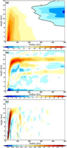
While it is not possible to construct a complete solution over the whole domain $[0,\infty )\times [0,H]$ by using the method of separation of variables, numerous modelling and observational studies have pointed out that hurricanes possess a very consistent structure as shown in Fig. 1. In particular, the hurricane wind field is always well defined with a distinct eyewall region where all components of the wind field attain their strongest amplitude after reaching the mature stage, provided that environmental conditions are favourable. This unique characteristic of the eyewall as shown in Fig. 1 suggests that it may be possible to construct a steady state that can describe the flows specifically inside the eyewall region.

A closer examination of the eyewall region reveals that the hurricane eyewall highly resembles an annulus of fluid whose boundaries are driven by strong rotational wind at the inner and outer edges. This observation leads to an idea of considering the eyewall as a fluid between two coaxial rotating cylinders in which the vertical motion w is upward, while the inner edge and outer edge rotate with different angular velocities such that the azimuthal wind v can approximately maintain its peak value across the annulus.

This focus on the eyewall domain is to some extent similar to previous approaches in which the hurricane domain is often divided into different regimes such that solutions in different regimes can be found (e.g. Anthes, 1974; Schubert and Hack, 1982; Schubert et al., 2007; Rozoff et al., 2008). One could in principle construct separate solutions for the inner-core and outer-core region and connect these solutions via smooth constraints. However, we will limit our search for solutions only for the eyewall region in this study due to the additional requirement of the stability analysis. Such a limitation to the eyewall solution leads to a strong constraint that the eyewall must be stirred by an external force to maintain its strong rotational wind inside the eyewall region. That is, the forcing term F_v in (6)(6) $$\frac{\partial v}{\partial t}+({\mathbf{u}}^{*}·\nabla )v+\frac{uv}{r}+fu=F_v,$$(6) must include a fictitious stirring force in addition to the physical frictional force to maintain the strong rotational wind within the isolated eyewall. To some extent, this fictitious force is equivalent to external azimuthal stresses applying at the inner and outer edges of a fluid between two co-axial rotating cylinders (e.g. Elliott, 1973). As a result of this eyewall separation, we consider a class of steady-state solutions for the eyewall region with the forces $(F_u,F_v,F_w)$ in Equations (5)–(7) of the following forms:(10) $$F_u=\nu \Delta u-\beta u,$$(10) (11) $$F_v=\nu \Delta v-\beta v+F_s,$$(11) (12) $$F_w=\nu \Delta w,$$(12) where F_s denotes the external stirring force needed to maintain the eyewall flow, $\Delta =\frac{{\partial }^2}{\partial r^2}+\frac{1}{r}\frac{\partial }{\partial r}+\frac{{\partial }^2}{\partial z^2}$ is the Laplace operator, $\beta >0$ is a coefficient that represents the surface linear drag similar to Stoke’s drag (e.g. Buizza, 1994) and ν denotes the atmospheric eddy viscosity.

While the external stirring term F_s in (11)(11) $$F_v=\nu \Delta v-\beta v+F_s,$$(11) appears to be mathematically arbitrary, it turns out that F_s must ensure several conditions such that the eyewall solution can be physically realized. These conditions are:

• it must be stationary to ensure the steady state solution, that is, $F_s\notin t$;

• it must not alter the functional form of the eyewall solution, that is, the functional forms of the solution u, v, w must be valid either in the presence or in the absence of F_s;

• it must be consistent with the rotational wind component v such that the stirring applied in the azimuthal direction can maintain the rotational wind.

These three conditions are sufficiently strong that the only functional form for F_s that could meet all three conditions are $F_s=A\hspace{0.17em}\text{cos}\hspace{0.17em}\frac{\lambda z}{2}$, where A > 0 is the amplitude of the stirring force and $\lambda \equiv \pi /H$. This specific functional form for F_s can be found by solving the system (5)–(7) with F_s = 0 as will be shown below. As such, we will hereinafter assume the external force $F_s=A\hspace{0.17em}\text{cos}\hspace{0.17em}\frac{\lambda z}{2}$ for the eyewall region.

Regarding the representation of the net diabatic heating term Q in Equation (9)(9) $$\frac{\partial \left(ru\right)}{\partial r}+\frac{\partial \left(r{w}^{*}\right)}{\partial z}+\frac{r{w}^{*}}{H}=0,$$(9) , this is a very challenging problem because the heating rate composes of various physical processes that are currently not fully understood such as radiative transfer, cloud physics, atmospheric gas concentration, aerosol or phase transition. Indeed, these processes are so complex that it is unlikely to find any functional form for the term heating Q. While a complete representation of this heating term is beyond our current knowledge, it happens in the eyewall region of hurricanes that the dominant diabatic heating term is proportional to the vertical motion (e.g. Liu et al., 1997; Zhang and Kieu, 2006). Thus, we will consider a simple parameterization in which the total diabatic heating term is the sum of a radiative cooling and the latent heat release due to the water phase change in the eyewall region. The former is roughly proportional to the buoyancy b according to the Newtonian relaxation process, while the latter is proportional to the vertical motion with the maximum value at the middle level and roughly equal to zero at the top and bottom boundaries. Mathematically, this heating function Q in the eyewall region can be therefore expressed as follows:(13) $$Q(r,z)=\delta w-\gamma b,$$(13) where the coefficient δ represents the efficiency of latent heat release feedback in the eyewall region of hurricanes, and γ is a coefficient for the Newtonian radiative cooling. Physically, (13)(13) $$Q(r,z)=\delta w-\gamma b,$$(13) states that a stronger vertical motion would promote more latent heating, thus resulting in larger latent heat release. Although this parameterization of the net diabatic heating is admittedly simple, it could at least capture the main features related to the diabatic heating and vertical motion in the eyewall region as often employed in previous hurricane models (see, e.g. Schubert and Hack, 1982; Schubert et al., 2007; Rozoff et al., 2008). For the stability analysis, it can be shown that the explicit functional form for Q turns out to be not critical, so long as this heating function is bounded as shown in Section 2.3.

Given the above parameterization for the net diabatic heating Q and the stirring force F_s, it is necessary to define the eyewall domain for our subsequent analyses. To be specific, the eyewall is defined hereinafter as an annulus region Ω around the RMW, which is given by (see the grey box in Fig. 1):(14) $$\Omega =\left\{\right(r,z\left)\right|0<z<H,r_1⩽r⩽r_2\},$$(14) where r₁ and r₂ denote the inner and outer radii of the eyewall annulus. For a typical hurricane, the range of the vertical coordinate $z\in (0,10\text{km})$, while $r_1\sim 20 \text{km}$ and $r_2\sim 30 \text{km}$, and so Ω is indeed a narrow annulus region. Unlike the realistic eyewall that tilts outwards with height (see Fig. 1), our eyewall domain Ω in this study has however no vertical tilting such that the boundaries $r_{1,2}$ do not depend on z. This approximation of an upright eyewall is certainly unrealistic, but it could at least reasonably capture the first-order structure of the eyewall for barotropic vortices that we can examine from the analytical perspective (see, e.g. Schubert and Hack, 1982; Schubert et al., 2007; Rozoff et al., 2008). With the unique property of the eyewall as shown in Fig. 1, we look for the solutions to (5)–(9) inside the eyewall annulus in the form (see, Kieu and Zhang, 2009):(15) $$\overline{u}(r,z)=-R\left(r\right)\lambda ·\hspace{0.17em}\text{cos}\hspace{0.17em}\lambda z,$$(15) (16) $$\overline{v}(r,z)=H\left(r\right)·\hspace{0.17em}\text{cos}\hspace{0.17em}\frac{\lambda }{2}z,$$(16) (17) $$\overline{w}(r,z)=\left(R\prime \left(r\right)+\frac{R\left(r\right)}{r}\right)·\hspace{0.17em}\text{sin}\hspace{0.17em}\lambda z,$$(17) where R(r) and H(r) are unknown functions required to ensure the consistency in the system (5)–(9). One first notices from the above functional forms for $\overline{u}$ and $\overline{w}$ that both $\overline{u}$ and $\overline{w}$ automatically satisfy the continuity Equation (9)(9) $$\frac{\partial \left(ru\right)}{\partial r}+\frac{\partial \left(r{w}^{*}\right)}{\partial z}+\frac{r{w}^{*}}{H}=0,$$(9) , provided that $w/H\ll \partial w/\partial z$ in the eyewall region (i.e. the flow is incompressible in the pseudo-height coordinate). While this Boussinesq approximation may appear to be too strict, we recall that the pseudo-height coordinate is just an alternate form of the isobaric coordinate in which the continuity equation is exactly divergent free (see Equation (4)(4) $$\nabla ·\mathbf{v}=0,$$(4) ). As such, the above functional forms for $\overline{u}$ and $\overline{w}$, which are exact in the isobaric coordinate, can be reasonably applied for the pseudo-height coordinate. As mentioned in Section 2.1, the use of the pseudo-height coordinate is preferred here simply because all variables have typical dimensions to facilitate our scale analyses later on. Thus, we will hereinafter assume the incompressible form for the eyewall region with a catch that an exact derivation can be always obtained by working directly in the isobaric coordinate such that no approximation will be needed.

Plugging (15)–(17) into Equation (6)(6) $$\frac{\partial v}{\partial t}+({\mathbf{u}}^{*}·\nabla )v+\frac{uv}{r}+fu=F_v,$$(6) with a note that$$\text{cos}\hspace{0.17em}\lambda z·\hspace{0.17em}\text{cos}\hspace{0.17em}\frac{\lambda }{2}z+\hspace{0.17em}\text{sin}\hspace{0.17em}\lambda z·\hspace{0.17em}\text{sin}\hspace{0.17em}\frac{\lambda }{2}z=\hspace{0.17em}\text{cos}\hspace{0.17em}\frac{\lambda }{2}z,$$

we obtain a relationship between R and H as follows:(18) $$\begin{array}{c}-\lambda R\left(H\prime +\frac{H}{r}\right)\hspace{0.17em}\text{cos}\hspace{0.17em}\lambda z·\hspace{0.17em}\text{cos}\hspace{0.17em}\frac{\lambda }{2}z\\ -\lambda \frac{H}{2}\left(R\prime +\frac{R}{r}\right)\hspace{0.17em}\text{sin}\hspace{0.17em}\lambda z·\hspace{0.17em}\text{sin}\hspace{0.17em}\frac{\lambda }{2}z\\ =\nu H″\hspace{0.17em}\text{cos}\hspace{0.17em}\frac{\lambda }{2}z+\nu \frac{H\prime }{r}\text{cos}\hspace{0.17em}\frac{\lambda }{2}z\\ -\frac{{\lambda }^2\nu }{4}H·\hspace{0.17em}\text{cos}\hspace{0.17em}\frac{\lambda }{2}z-\beta H·\hspace{0.17em}\text{cos}\hspace{0.17em}\frac{\lambda }{2}z+A\hspace{0.17em}\text{cos}\hspace{0.17em}\frac{\lambda }{2}z,\end{array}$$(18) where the Coriolis force in the eyewall region is neglected. To find the solution of Equation (18)(18) $$\begin{array}{c}-\lambda R\left(H\prime +\frac{H}{r}\right)\hspace{0.17em}\text{cos}\hspace{0.17em}\lambda z·\hspace{0.17em}\text{cos}\hspace{0.17em}\frac{\lambda }{2}z\\ -\lambda \frac{H}{2}\left(R\prime +\frac{R}{r}\right)\hspace{0.17em}\text{sin}\hspace{0.17em}\lambda z·\hspace{0.17em}\text{sin}\hspace{0.17em}\frac{\lambda }{2}z\\ =\nu H″\hspace{0.17em}\text{cos}\hspace{0.17em}\frac{\lambda }{2}z+\nu \frac{H\prime }{r}\text{cos}\hspace{0.17em}\frac{\lambda }{2}z\\ -\frac{{\lambda }^2\nu }{4}H·\hspace{0.17em}\text{cos}\hspace{0.17em}\frac{\lambda }{2}z-\beta H·\hspace{0.17em}\text{cos}\hspace{0.17em}\frac{\lambda }{2}z+A\hspace{0.17em}\text{cos}\hspace{0.17em}\frac{\lambda }{2}z,\end{array}$$(18) , we observe that the functional form on both sides of (18)(18) $$\begin{array}{c}-\lambda R\left(H\prime +\frac{H}{r}\right)\hspace{0.17em}\text{cos}\hspace{0.17em}\lambda z·\hspace{0.17em}\text{cos}\hspace{0.17em}\frac{\lambda }{2}z\\ -\lambda \frac{H}{2}\left(R\prime +\frac{R}{r}\right)\hspace{0.17em}\text{sin}\hspace{0.17em}\lambda z·\hspace{0.17em}\text{sin}\hspace{0.17em}\frac{\lambda }{2}z\\ =\nu H″\hspace{0.17em}\text{cos}\hspace{0.17em}\frac{\lambda }{2}z+\nu \frac{H\prime }{r}\text{cos}\hspace{0.17em}\frac{\lambda }{2}z\\ -\frac{{\lambda }^2\nu }{4}H·\hspace{0.17em}\text{cos}\hspace{0.17em}\frac{\lambda }{2}z-\beta H·\hspace{0.17em}\text{cos}\hspace{0.17em}\frac{\lambda }{2}z+A\hspace{0.17em}\text{cos}\hspace{0.17em}\frac{\lambda }{2}z,\end{array}$$(18) suggests us to search for R and H that satisfy the following relationship:(19) $$\begin{array}{c}\lambda R\left(H\prime +\frac{H}{r}\right)=\lambda \frac{H}{2}\left(R\prime +\frac{R}{r}\right)\hfill \\ \hfill & =\frac{{\lambda }^2\nu }{4}H+\beta H-A-H″-\frac{H\prime }{r}.\hfill \end{array}$$(19)

A quick inspection of this condition confirms that (18)(18) $$\begin{array}{c}-\lambda R\left(H\prime +\frac{H}{r}\right)\hspace{0.17em}\text{cos}\hspace{0.17em}\lambda z·\hspace{0.17em}\text{cos}\hspace{0.17em}\frac{\lambda }{2}z\\ -\lambda \frac{H}{2}\left(R\prime +\frac{R}{r}\right)\hspace{0.17em}\text{sin}\hspace{0.17em}\lambda z·\hspace{0.17em}\text{sin}\hspace{0.17em}\frac{\lambda }{2}z\\ =\nu H″\hspace{0.17em}\text{cos}\hspace{0.17em}\frac{\lambda }{2}z+\nu \frac{H\prime }{r}\text{cos}\hspace{0.17em}\frac{\lambda }{2}z\\ -\frac{{\lambda }^2\nu }{4}H·\hspace{0.17em}\text{cos}\hspace{0.17em}\frac{\lambda }{2}z-\beta H·\hspace{0.17em}\text{cos}\hspace{0.17em}\frac{\lambda }{2}z+A\hspace{0.17em}\text{cos}\hspace{0.17em}\frac{\lambda }{2}z,\end{array}$$(18) will be indeed an identity if (19)(19) $$\begin{array}{c}\lambda R\left(H\prime +\frac{H}{r}\right)=\lambda \frac{H}{2}\left(R\prime +\frac{R}{r}\right)\hfill \\ \hfill & =\frac{{\lambda }^2\nu }{4}H+\beta H-A-H″-\frac{H\prime }{r}.\hfill \end{array}$$(19) is satisfied. Dividing (19)(19) $$\begin{array}{c}\lambda R\left(H\prime +\frac{H}{r}\right)=\lambda \frac{H}{2}\left(R\prime +\frac{R}{r}\right)\hfill \\ \hfill & =\frac{{\lambda }^2\nu }{4}H+\beta H-A-H″-\frac{H\prime }{r}.\hfill \end{array}$$(19) by $RH\lambda$ results in a pair of constraints as follows:(20) $$\left(\frac{H\prime }{H}+\frac{1}{r}\right)=\frac{1}{2}\left(\frac{R\prime }{R}+\frac{1}{r}\right),$$(20) (21) $$\begin{array}{cc}\left(\frac{H\prime }{H}+\frac{1}{r}\right)=\hfill & \frac{\lambda \nu }{4R}+\frac{\beta }{\lambda R}-\frac{A}{RH\lambda }-\frac{\nu H″}{RH\lambda }-\frac{\nu H\prime }{rRH\lambda }.\hfill \end{array}$$(21)

The steady-state solution can now be directly derived from (20)–(21). Indeed, we note that the simplest choice for the function H is(22) $$H=V_0, \text{where} V_0 \text{is} \text{constant} .$$(22)

Hence, (20)(20) $$\left(\frac{H\prime }{H}+\frac{1}{r}\right)=\frac{1}{2}\left(\frac{R\prime }{R}+\frac{1}{r}\right),$$(20) leads to(23) $$R=W_{0}r,$$(23) where W₀ is another constant that satisfies(24) $$W_0=\frac{\lambda \nu }{4}+\frac{\beta }{\lambda }-\frac{A}{V_0\lambda }.$$(24)

Thus, a complete steady-state solution for the hurricane wind structure in the eyewall region Ω that ensures (5)–(9) is given by(25) $$\overline{u}(r,z)=-W_0\lambda r·\hspace{0.17em}\text{cos}\hspace{0.17em}\lambda z,$$(25) (26) $$\overline{v}\left(z\right)=V_0·\hspace{0.17em}\text{cos}\hspace{0.17em}\frac{\lambda }{2}z,$$(26) (27) $$\overline{w}\left(z\right)=2W_0·\hspace{0.17em}\text{sin}\hspace{0.17em}\lambda z$$(27) $$\forall (r,z)\in \Omega .$$

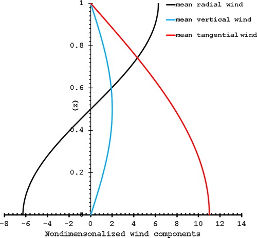
Figure 2 shows the vertical structure of the solutions (25)–(27), which are averaged over the eyewall region Ω, assuming the typical values of the hurricane winds at the mature stage. As expected, the eyewall tangential wind is indeed dominantly cyclonic (i.e. v(z) > 0) at all levels, while the vertical motion peaks at the middle level and approaches zero at the surface and top boundary similar to that in a typical mature storm (cf. Fig. 1). Likewise, the radial wind shows a large inflow in the lower half of the troposphere along with an outflow at the upper levels.

Fig. 2. The vertical profiles of the non-dimensionalized steady-state solution (25)–(27) as a function of z, which are averaged over the whole eyewall region. The non-dimensionalization assumes the eyewall domain given by $r_1=18\text{km}$ and $r_2=20\text{km}$, the maximum azimuthal wind at the surface $V_0=70{\mathrm{m} \mathrm{s}}^{-1}$, the maximum vertical motion $W_0=2{\mathrm{m} \mathrm{s}}^{-1}$, and the scale height $H=10\text{km}$.

As can be seen from the above derivations, the general forms of the steady state given by (15)–(17) turn out to be valid even in the absence of the fictitious stirring term $A\hspace{0.17em}\text{cos}(\lambda z/2)$ in (11)(11) $$F_v=\nu \Delta v-\beta v+F_s,$$(11) , that is, when A = 0. This is an important point, because it indicates that the functional form of the solution (15)–(17) is generic, regardless of the amplitude of the fictitious forcing as emphasized above. From this perspective, the functional form of the stirring term F_s cannot be arbitrary, but it must take the form of $A\hspace{0.17em}\text{cos}(\lambda z/2)$ to accord with the solution (15)–(17) in the eyewall region. This consistency of F_s and the rotational wind component v justifies our choice of the stirring term in the form of $A\hspace{0.17em}\text{cos}(\lambda z/2)$ for the forcing term F_s.

Although the steady-state solutions (25)–(27) could capture the broad feature of the eyewall wind field, more careful comparison of this solution with the actual model output shown in Fig. 1 shows that the exact solution has some inconsistency near the surface. Specifically, the typical tangential wind of a real mature storm should approach to zero at z = 0 (cf. Fig. 1), whereas the profile (26)(26) $$\overline{v}\left(z\right)=V_0·\hspace{0.17em}\text{cos}\hspace{0.17em}\frac{\lambda }{2}z,$$(26) gives the largest magnitude at the surface. This discrepancy is attributed to the simplified PBL frictional force $F_{(u,v)}$ assumed in this study, which is given by (10)–(11). In practice, the eddy coefficient ν is much larger within the PBL near the surface layer, and rapidly approaches zero above the PBL. Thus, assuming a constant value for ν reduces the direct impacts of friction, and results in unexpected behaviours of the steady-state solution (26)(26) $$\overline{v}\left(z\right)=V_0·\hspace{0.17em}\text{cos}\hspace{0.17em}\frac{\lambda }{2}z,$$(26) at z = 0.

A more realistic representation for the eddy coefficient ν would require a closure that involves details of turbulent kinetic energy that does not currently possess any analytical form, and so it is beyond the analytical approach presented in this study (e.g. Bryan and Rotunno, 2009). Alternatively, one can treat friction as a perturbation parameter of a serial expansion such that a better wind profile in the PBL can be obtained Kieu and Zhang (2009). However, this serial expansion approach does not always guarantee the convergence of the series when friction is sufficiently large and so it is also not presented herein. As a result of the simple friction treatment, the steady-state solution (25)–(27) appears to be therefore more applicable for the hurricane eyewall in the free atmosphere above the PBL rather than for the entire troposphere. Despite this drastic simplification of the PBL eddy representation, that the solution (25)–(27) could capture the overall structure of the eyewall wind field above the PBL is of significance, because it indicates the existence of a consistent wind structure among all components of the wind field at the mature stage. Whether this eyewall structure is stable or not is examined in the next section.

We note that the above class of the steady-state solutions for the hurricane eyewall requires four free parameters to fully determine the solutions, which include the tangential wind amplitude V₀ at z = 0, the scale of the tropospheric depth $\lambda \sim 1/H$, the surface drag parameter β and the viscosity coefficient ν. All other parameters must be constrained by the stability and physical representation of the solution, once these free parameters are given. Among the above four free parameters, we remark that V₀ represents the maximum intensity that a hurricane can achieve in a given environmental condition at the surface. As such, V₀ technically corresponds to the MPI limit near the surface as dictated by Emanuel’s theory. Because our focus in this study is on the full structure of the steady-state solution and its stability in the eyewall rather than a single maximum value for the MPI at the surface, V₀ will be therefore treated as a given parameter as dictated by Emanuel’s MPI formulation.

By further substituting (25)–(27) into (5)(5) $$\frac{\partial u}{\partial t}+({\mathbf{u}}^{*}·\nabla )u-\frac{v^2}{r}-fv=-{\varphi }_r+F_u,$$(5) and (9)(9) $$\frac{\partial \left(ru\right)}{\partial r}+\frac{\partial \left(r{w}^{*}\right)}{\partial z}+\frac{r{w}^{*}}{H}=0,$$(9) , it is possible to construct a complete set of the steady-state solutions for the remaining variables $\varphi$ and b consistent with the system (5)–(9) (Kieu and Zhang, 2010). In this regard, one can construct a pressure distribution in balance with the given azimuthal wind distribution as expected from the balance theory, except for the existence of the vertical wind in the eyewall. Of course this horizontal wind balance differs from the typical gradient wind balance due to the contribution from the radial advection. Nevertheless, the pressure distribution would be very close to that obtained from the gradient wind balance due to the dominance of the $v^2/r$ term. Because the explicit forms of $\varphi$ and b are not needed for our subsequent stability analysis in the eyewall region, the complete balance solution for $\varphi$ and b are not provided hereinafter.

2.3. Nonlinear stability analysis

Among several techniques to understand the stability of a dynamical system, the normal mode linear expansion approach that transforms a partial differential equation (PDE) problem to an ordinary differential equation (ODE) system for perturbations seems to be the most common method in the stability study. This method is widely applied to study the hydrodynamic and geophysical problems, because it allows for obtaining a spectrum of eigenvalues of a corresponding linear differential operator and related stability (e.g. Chandrasekhar, 1961). While the normal mode approach is generally useful to deal with linear stability problems, one of its caveats is that a steady state must depend on one coordinate variable, and the corresponding stability has to be local due to neglecting nonlinear terms. As a consequence, this method is not suitable to analyze the linear stability of our steady-state (25)–(27) due to the dependence of this solution on both the coordinate variables r and z.

A second approach that is also effective for studying the stability of fluid systems is the energy method. Unlike the normal mode approach, the energy method does not require exact expressions of the steady state (Serrin, 1959; Joseph, 1965). Specifically, the energy method relies on an estimation of perturbation energy around a given steady state, and requires that the perturbation energy must be damped with time such that the steady state can be maintained. The examination of the perturbation energy is especially useful in the case when the stability and convergence of the steady state solution is of more concern than the specific functional forms of these solutions. Examples of such a situation are proofs of the convergence of solutions to the Navier–Stoke equations towards the Euler equations when $\nu \to 0$, or the smooth dependence of a solution on the initial conditions. Although the energy method is not as widely used as the normal mode method, it is a more practical approach for the hurricane stability problem, because the complete solutions for all variables are not needed as seen below (e.g. Straughan, 2004).

To analyze the stability of the steady-state eyewall solution (25)–(27) based on the energy method, we first develop an equation for the perturbation energy E, which is defined as(28) $$E\left(t\right)={\int }_{r_1}^{r_2}{\int }_0^H(S{\mathbf{u}}^2+b^2)\mathrm{d}\tau ,$$(28) where $\mathrm{d}\tau \equiv r\mathrm{d}r\mathrm{d}z$, and then show that(29) $$\frac{\mathrm{d}E\left(t\right)}{\mathrm{d}t}⩽-C_{0}E\left(t\right), E\left(0\right)=E_0,$$(29) for a positive constant C₀ and initial perturbation energy E₀. Physically, (29)(29) $$\frac{\mathrm{d}E\left(t\right)}{\mathrm{d}t}⩽-C_{0}E\left(t\right), E\left(0\right)=E_0,$$(29) implies that the perturbation energy E(t) will exponentially decay with time as expected for a stable system. To this end, denote the perturbation fields as $\mathbf{u}\prime =(u\prime ,v\prime ,w\prime )$, and substitute $\mathbf{u}=(u,v,w)=\mathbf{u}\prime +\overline{\mathbf{u}}$ into Equations (5)–(9) to arrive at a set of perturbation equations as follows:(30) $$\begin{array}{cc}\hfill & \frac{\partial u}{\partial t}+(\overline{\mathbf{u}}·\nabla )u+(\mathbf{u}·\nabla )\overline{u}+(\mathbf{u}·\nabla )u\hfill \\ \hfill & -\frac{v^2}{r}-\frac{2\overline{v}v}{r}=-{\varphi }_r+\nu \Delta u-\beta u,\hfill \end{array}$$(30) (31) $$\begin{array}{cc}\hfill & \frac{\partial v}{\partial t}+(\overline{\mathbf{u}}·\nabla )v+(\mathbf{u}·\nabla )\overline{v}+(\mathbf{u}·\nabla )v\hfill \\ \hfill & +\frac{vu}{r}+\frac{\overline{v}u+\overline{u}v}{r}=\nu \Delta v-\beta v,\hfill \end{array}$$(31) (32) $$\begin{array}{cc}\hfill & \frac{\partial w}{\partial t}+(\overline{\mathbf{u}}·\nabla )w+(\mathbf{u}·\nabla )\overline{w}+(\mathbf{u}·\nabla )w\hfill \\ \hfill & =-{\varphi }_z+\nu \Delta w-\beta w+b,\hfill \end{array}$$(32) (33) $$\begin{array}{cc}\hfill & \frac{\partial b}{\partial t}+(\overline{\mathbf{u}}·\nabla )b+(\mathbf{u}·\nabla )\overline{b}+(\mathbf{u}·\nabla )b\hfill \\ \hfill & +sw=-\gamma b+\delta v\hspace{0.17em}\text{sin}\hspace{0.17em}\lambda z,\hfill \end{array}$$(33) (34) $$\frac{\partial \left(ru\right)}{\partial r}+\frac{\partial \left(rw\right)}{\partial z}=0,$$(34) where the primes have been dropped hereinafter for the sake of convenience, and(35) $$\begin{array}{c}(A·\nabla )B=A_1\frac{\partial \mathbf{B}}{\partial r}+A_3\frac{\partial \mathbf{B}}{\partial z},\\ A=(A_1,A_2,A_3),B=(B_1,B_2,B_3).\end{array}$$(35)

Unlike the linear stability method in which the linearization around the steady state is required, it should be mentioned that the full nonlinearity is retained in the above perturbation form. In what follows, we will show that there exists an inequality (29)(29) $$\frac{\mathrm{d}E\left(t\right)}{\mathrm{d}t}⩽-C_{0}E\left(t\right), E\left(0\right)=E_0,$$(29) for the energy functional defined by (28)(28) $$E\left(t\right)={\int }_{r_1}^{r_2}{\int }_0^H(S{\mathbf{u}}^2+b^2)\mathrm{d}\tau ,$$(28) relative to our steady-state (25)–(27).

Indeed, multiplying (30)–(32) by u and integrating over the whole eyewall domain Ω, we have(36) $$\begin{array}{c}\frac{1}{2}\frac{\mathrm{d}}{\mathrm{d}t}{\int }_{r_1}^{r_2}{\int }_0^H{\mathbf{u}}^2\mathrm{d}\tau \\ +{\int }_{r_1}^{r_2}{\int }_0^H\left(\right(\overline{\mathbf{u}}·\nabla )\mathbf{u}·\mathbf{u}+(\mathbf{u}·\nabla )\overline{\mathbf{u}}·\mathbf{u}\end{array}$$(36) (37) $$\begin{array}{c}+(\mathbf{u}·\nabla )\mathbf{u}·\mathbf{u}+\frac{\overline{u}{v}^2-\overline{v}vu}{r})\mathrm{d}\tau \\ ={\int }_{r_1}^{r_2}{\int }_0^H(-\beta {\mathbf{u}}^2-\nu ({\left(r\frac{\partial \mathbf{u}}{\partial r}\right)}^2+{\left(\frac{\partial \mathbf{u}}{\partial z}\right)}^2)\end{array}$$(37) (38) $$-u{\varphi }_r-w{\varphi }_z+bw)\mathrm{d}\tau .$$(38)

A similar procedure for the thermodynamic Equation (8)(8) $$\frac{\partial b}{\partial t}+({\mathbf{u}}^{*}·\nabla )b+S{w}^{*}=Q,$$(8) results in(39) $$\begin{array}{c}\frac{1}{2}\frac{\mathrm{d}}{\mathrm{d}t}{\int }_{r_1}^{r_2}{\int }_0^H{b}^2\mathrm{d}\tau \\ +{\int }_{r_1}^{r_2}{\int }_0^H\left(\right(\overline{\mathbf{u}}·\nabla )b·b+(\mathbf{u}·\nabla )\overline{b}·b\end{array}$$(39) (40) $$+(\mathbf{u}·\nabla )b·b)\mathrm{d}\tau$$(40) (41) $$={\int }_{r_1}^{r_2}{\int }_0^H(-\gamma b^2+\delta wb-\mathrm{S}wb)\mathrm{d}\tau .$$(41)

Consider next a class of perturbation fields $(\mathbf{u},b)$ that satisfy the following homogeneous boundary conditions at the inner and outer edges of the annulus(42) $$\begin{array}{cc}\hfill & \left(u\right(r_1,z),v(r_1,z),w(r_1,z\left)\right)=(0,0,0),\hfill \\ \hfill & \left(u\right(r_2,z),v(r_2,z),w(r_2,z\left)\right)=(0,0,0),\hfill \\ \hfill & \left(u\right(r,0),v(r,0),w(r,0\left)\right)=(0,0,0),\hfill \\ \hfill & \left(u\right(r,H),v(r,H),w(r,H\left)\right)=(0,0,0),\hfill \\ \hfill & b(r_1,z)=b(r_2,z)=0,b(r,0)=b(r,H)=0,\hfill \end{array}$$(42) we then obtain(43) $$\begin{array}{cc}& {\int }_{r_1}^{r_2}{\int }_0^H(\overline{\mathbf{u}}·\nabla )\mathbf{u}·\mathbf{u}\mathrm{d}\tau =0,\\ & {\int }_{r_1}^{r_2}{\int }_0^H(\mathbf{u}·\nabla )\mathbf{u}·\mathbf{u}\mathrm{d}\tau =0,\\ & {\int }_{r_1}^{r_2}{\int }_0^H(\overline{\mathbf{u}}·\nabla )b·b\mathrm{d}\tau =0,\\ & {\int }_{r_1}^{r_2}{\int }_0^H(\mathbf{u}·\nabla )b·b\mathrm{d}\tau =0.\end{array}$$(43)

Physically, the boundary conditions (42)(42) $$\begin{array}{cc}\hfill & \left(u\right(r_1,z),v(r_1,z),w(r_1,z\left)\right)=(0,0,0),\hfill \\ \hfill & \left(u\right(r_2,z),v(r_2,z),w(r_2,z\left)\right)=(0,0,0),\hfill \\ \hfill & \left(u\right(r,0),v(r,0),w(r,0\left)\right)=(0,0,0),\hfill \\ \hfill & \left(u\right(r,H),v(r,H),w(r,H\left)\right)=(0,0,0),\hfill \\ \hfill & b(r_1,z)=b(r_2,z)=0,b(r,0)=b(r,H)=0,\hfill \end{array}$$(42) imply that all perturbations would be largest inside the eyewall and quickly damped near the edges of the eyewall. This assumption is not unrealistic if one notes that the most vigorous convection often takes place within the eyewall region, which encloses a calm eye inside and is surrounded by a moat area outside (cf. Fig. 1). One could in principle impose less strict boundary conditions by simply requiring that the fluxes of the perturbation energy are cancelled at the boundaries or using other combination of more complex boundary conditions. A variational approach discussed in Section 3 outlines a procedure to handle more general types of boundary conditions, but this requires numerical approach that is beyond our analytical analyses and will not be pursued further. With the above boundary conditions (43)(43) $$\begin{array}{cc}& {\int }_{r_1}^{r_2}{\int }_0^H(\overline{\mathbf{u}}·\nabla )\mathbf{u}·\mathbf{u}\mathrm{d}\tau =0,\\ & {\int }_{r_1}^{r_2}{\int }_0^H(\mathbf{u}·\nabla )\mathbf{u}·\mathbf{u}\mathrm{d}\tau =0,\\ & {\int }_{r_1}^{r_2}{\int }_0^H(\overline{\mathbf{u}}·\nabla )b·b\mathrm{d}\tau =0,\\ & {\int }_{r_1}^{r_2}{\int }_0^H(\mathbf{u}·\nabla )b·b\mathrm{d}\tau =0.\end{array}$$(43) , Equations (37)–(41) can be now rewritten as(44) $$\begin{array}{cc}& \frac{1}{2}\frac{\mathrm{d}}{\mathrm{d}t}{\int }_{r_1}^{r_2}{\int }_0^H{\mathbf{u}}^2\mathrm{d}\tau \\ & +{\int }_{r_1}^{r_2}{\int }_0^H\left(\right(\mathbf{u}·\nabla )\overline{\mathbf{u}}·\mathbf{u}+\frac{\overline{u}{v}^2-\overline{v}vu}{r})\mathrm{d}\tau \\ & ={\int }_{r_1}^{r_2}{\int }_0^H(-\beta {\mathbf{u}}^2+bw\\ & -\nu ({\left(r\frac{\partial \mathbf{u}}{\partial r}\right)}^2+{\left(\frac{\partial \mathbf{u}}{\partial z}\right)}^2))\mathrm{d}\tau ,\end{array}$$(44) (45) $$\begin{array}{cc}& \frac{1}{2}\frac{\mathrm{d}}{\mathrm{d}t}{\int }_{r_1}^{r_2}{\int }_0^b{b}^2\mathrm{d}\tau +{\int }_{r_1}^{r_2}{\int }_0^H(\mathbf{u}·\nabla )\overline{b}·b \mathrm{d}x\\ & ={\int }_{r_1}^{r_2}{\int }_0^H(-\gamma b^2+\delta wb-\mathrm{S}wb)\mathrm{d}x\tau .\end{array}$$(45)

If we note further that(46) $$\begin{array}{c}(u·\nabla )\overline{\mathbf{u}}·u+\frac{\overline{u}{v}^2-\overline{v}vu}{r}\\ =(u,v,w)\left(\begin{array}{ccc}\frac{\partial \overline{u}}{\partial r}& -\frac{\overline{v}}{2r}& \frac{1}{2}\frac{\partial \overline{u}}{\partial z}\\ -\frac{\overline{v}}{2r}& \frac{\overline{u}}{r}& \frac{1}{2}\frac{\partial \overline{v}}{\partial z}\\ \frac{1}{2}\frac{\partial \overline{u}}{\partial z}& \frac{1}{2}\frac{\partial \overline{v}}{\partial z}& \frac{\partial \overline{w}}{\partial z}\end{array}\right)\left(\begin{array}{c}u\\ v\\ w\end{array}\right)\\ =(u,v,w)A{(u,v,w)}^T,\end{array}$$(46) where$$\mathbf{A}=\left(\begin{array}{ccc}-W_0\lambda \text{cos}\lambda z& -\frac{V_0\text{cos}\frac{\lambda }{2}z}{2r}& \frac{W_{0}r{\lambda }^2}{2}\text{sin}\lambda z\\ -\frac{V_0\text{cos}\frac{\lambda }{2}z}{2r}& -W_0\lambda \text{cos}\lambda z& -\frac{V_0\lambda }{4}\text{sin}\frac{\lambda }{2}z\\ \frac{W_{0}r{\lambda }^2}{2}\text{sin}\lambda z& -\frac{V_0\lambda }{4}\text{sin}\frac{\lambda }{2}z& 2W_0\lambda \text{cos}\lambda z\end{array}\right).$$

It is then straightforward to see from this quadratic form that(47) $$\begin{array}{cc}& {\int }_{r_1}^{r_2}{\int }_0^H\left(\right(\mathbf{u}·\nabla )\overline{\mathbf{u}}·\mathbf{u}+\frac{\overline{u}{v}^2-\overline{v}vu}{r})\mathrm{d}\tau \\ & ={\int }_{r_1}^{r_2}{\int }_0^H(u,v,w)A{(u,v,w)}^T\mathrm{d}\tau \\ & ⩾-W^{*}\lambda {\int }_{r_1}^{r_2}{\int }_0^H{\mathbf{u}}^2\mathrm{d}\tau .\end{array}$$(47)

Here, $-W^{*}$ is the minimum value of the lowest eigenvalue of the following matrix:$$M(r,z)=\frac{1}{\lambda }\mathbf{A},$$and we have used a property that$$\begin{array}{c}(u,v,w)A{(u,v,w)}^T\\ =\lambda (u,v,w)M(r,z){(u,v,w)}^T⩾-W^{*}\lambda {\mathbf{u}}^2.\end{array}$$

If we denote the lowest eigenvalue of M(r, z) as $\eta (r,z)$, and let(48) $$\xi \left(r\right)=\underset{{}_{0⩽z⩽H}}{\min }\eta (r,z),$$(48) then $-W^{*}$ is given more precisely as$$-W^{*}=\underset{{}_{r_1⩽r⩽r_2}}{\min }\xi \left(r\right).$$

With the definition of $W^{*}$ as the lowest bound, we then obtain a particular constraint among $W^{*},W_0,V_0$ by noting that the above matrix M(r, z) at z = 0 is$$M(V_0,W_0,r,0)=\left(\begin{array}{ccc}-W_0& -\frac{V_0}{2\lambda r}& 0\\ -\frac{V_0}{2\lambda r}& -W_0& 0\\ 0& 0& 2W_0\end{array}\right),$$whose eigenvalues are, respectively, given by$${\eta }_1=2W_0, {\eta }_2=-W_0+\frac{V_0}{2\lambda r}, {\eta }_3=-W_0-\frac{V_0}{2\lambda r}.$$

Thus, the parameter $W^{*},W_0,V_0$ must satisfy the following condition:(49) $$W^{*}⩾W_0+\frac{V_0}{2\lambda r}.$$(49)

Basically, (49)(49) $$W^{*}⩾W_0+\frac{V_0}{2\lambda r}.$$(49) indicates that the dependence of the stability of the eyewall solution will impose a constraint on $W^{*},W^0,V^0$. Because of the estimation (47)(47) $$\begin{array}{cc}& {\int }_{r_1}^{r_2}{\int }_0^H\left(\right(\mathbf{u}·\nabla )\overline{\mathbf{u}}·\mathbf{u}+\frac{\overline{u}{v}^2-\overline{v}vu}{r})\mathrm{d}\tau \\ & ={\int }_{r_1}^{r_2}{\int }_0^H(u,v,w)A{(u,v,w)}^T\mathrm{d}\tau \\ & ⩾-W^{*}\lambda {\int }_{r_1}^{r_2}{\int }_0^H{\mathbf{u}}^2\mathrm{d}\tau .\end{array}$$(47) , Equations (44)–(45) can be rearranged as follows:$$\begin{array}{cc}& \frac{1}{2}\frac{\mathrm{d}}{\mathrm{d}t}{\int }_{r_1}^{r_2}{\int }_0^H(S{\mathbf{u}}^2+b^2+(\mathbf{u}·\nabla )\overline{b}·b)\mathrm{d}x\\ & ⩽{\int }_{r_1}^{r_2}{\int }_0^H(-S\beta {\mathbf{u}}^2+S{W}^{*}\lambda {\mathbf{u}}^2-\gamma b^2+\delta wb)\mathrm{d}x\\ & -S\nu {\int }_{r_1}^{r_2}{\int }_0^H({\left(r\frac{\partial \mathbf{u}}{\partial r}\right)}^2+{\left(\frac{\partial \mathbf{u}}{\partial z}\right)}^2)\mathrm{d}\tau .\end{array}$$

By the Dirichlet–Poincare inequality(50) $$\begin{array}{cc}& {\int }_{r_1}^{r_2}{\int }_0^H({\left(r\frac{\partial \mathbf{u}}{\partial r}\right)}^2+{\left(\frac{\partial \mathbf{u}}{\partial z}\right)}^2)\mathrm{d}x\\ & ⩾\Gamma {\int }_{r_1}^{r_2}{\int }_0^H{\mathbf{u}}^2\mathrm{d}x,\end{array}$$(50) where Γ is large or equal to $\min \left\{\frac{1}{{(r_2-r_1)}^2},\frac{1}{H^2}\right\}$, and the Cauchy inequality(51) $${\int }_{r_1}^{r_2}{\int }_0^{H}wb\mathrm{d}x⩽\frac{1}{2}{\int }_{r_1}^{r_2}{\int }_0^H(w^2+b^2)\mathrm{d}\tau ,$$(51) (52) $$|{\int }_{r_1}^{r_2}{\int }_0^H(\mathbf{u}·\nabla )\overline{b}·b\mathrm{d}\tau |⩽\frac{\Lambda }{2}{\int }_{r_1}^{r_2}{\int }_0^H({\mathbf{u}}^2+b^2)\mathrm{d}\tau ,$$(52) where $\Lambda ⩽\max (|\nabla \overline{b}|)$, we finally arrive at an equation governing the growth rate of the perturbation energy around the steady-state solution in the eyewall region:(53) $$\begin{array}{cc}& \frac{1}{2}\frac{\mathrm{d}}{\mathrm{d}t}{\int }_{r_1}^{r_2}{\int }_0^H(S{\mathbf{u}}^2+b^2)\mathrm{d}x\\ & ⩽{\int }_{r_1}^{r_2}{\int }_0^H(-S\beta {\mathbf{u}}^2+S{W}^{*}\lambda {\mathbf{u}}^2\\ & -S\nu \Gamma u^2-\gamma b^2+\frac{\Lambda +\delta }{2}{\mathbf{u}}^2+\frac{\Lambda +\delta }{2}{b}^2)\mathrm{d}x.\end{array}$$(53)

In general, it is not possible to conclude anything about the rate of change of the perturbation energy as given by (53)(55) $$\begin{array}{cc}& \frac{1}{2}\frac{\mathrm{d}}{\mathrm{d}t}{\int }_{r_1}^{r_2}{\int }_0^H(S{\mathbf{u}}^2+b^2)\mathrm{d}x\\ & ⩽-C{\int }_{r_1}^{r_2}{\int }_0^H(S{\mathbf{u}}^2+b^2)\mathrm{d}x<0.\end{array}$$(55) due to different contributions from various terms on the right hand side of (52)(52) $$|{\int }_{r_1}^{r_2}{\int }_0^H(\mathbf{u}·\nabla )\overline{b}·b\mathrm{d}\tau |⩽\frac{\Lambda }{2}{\int }_{r_1}^{r_2}{\int }_0^H({\mathbf{u}}^2+b^2)\mathrm{d}\tau ,$$(52) . One notices, however, that if the right hand side of (52)(52) $$|{\int }_{r_1}^{r_2}{\int }_0^H(\mathbf{u}·\nabla )\overline{b}·b\mathrm{d}\tau |⩽\frac{\Lambda }{2}{\int }_{r_1}^{r_2}{\int }_0^H({\mathbf{u}}^2+b^2)\mathrm{d}\tau ,$$(52) satisfies the following conditions:(54) $$\begin{array}{cc}\hfill & S{W}^{*}\lambda +\frac{\Lambda +\delta }{2}<S(\beta +\nu \Gamma ),\hfill \\ \hfill & \frac{\Lambda +\delta }{2}<\gamma , S\ne 0,A⩾0,\hfill \end{array}$$(54) it is then simple to obtain an expected inequality for the growth rate of the perturbation energy as:(55) $$\begin{array}{cc}& \frac{1}{2}\frac{\mathrm{d}}{\mathrm{d}t}{\int }_{r_1}^{r_2}{\int }_0^H(S{\mathbf{u}}^2+b^2)\mathrm{d}x\\ & ⩽-C{\int }_{r_1}^{r_2}{\int }_0^H(S{\mathbf{u}}^2+b^2)\mathrm{d}x<0.\end{array}$$(55)

Physically, the condition (55)(55) $$\begin{array}{cc}& \frac{1}{2}\frac{\mathrm{d}}{\mathrm{d}t}{\int }_{r_1}^{r_2}{\int }_0^H(S{\mathbf{u}}^2+b^2)\mathrm{d}x\\ & ⩽-C{\int }_{r_1}^{r_2}{\int }_0^H(S{\mathbf{u}}^2+b^2)\mathrm{d}x<0.\end{array}$$(55) implies that any perturbations triggered within the eyewall region will be damped over time, thus proving nonlinear stability of the steady-state eyewall structure given by (25)–(27). This proof of the stability of the hurricane eyewall is consistent with previous modelling studies of hurricane development, which always capture a stable quasi-stationary state of the hurricane eyewall at the peak intensity so long as favourable environmental conditions are maintained. We note that unlike the inertial stability associated with the horizontal displacement around a given balanced vortex, the eyewall nonlinear stability presented herein deals with a full 3D structure that includes all advective terms, frictional effects as well as the thermodynamic contribution. As seen in the above proof, such nonlinear stability is possible mostly because of the frictional effects that dissipate the perturbation energy with time, which is typically applied in dissipative dynamical systems. In this regard, our proof of the eyewall stability is general and not subject to the limit of the pure horizontal flows as constrained by the balance vortex structure.

3. Discussions

While the preceding section could demonstrate the existence and the nonlinear stability of the steady-state solution (25)–(27) for the eyewall region, several issues remain. Specifically, one must examine under what physical conditions the eyewall solution (25)–(27) can exist, or whether the inequality (54)(54) $$\begin{array}{cc}\hfill & S{W}^{*}\lambda +\frac{\Lambda +\delta }{2}<S(\beta +\nu \Gamma ),\hfill \\ \hfill & \frac{\Lambda +\delta }{2}<\gamma , S\ne 0,A⩾0,\hfill \end{array}$$(54) can be realized in practice so that the stability proof is valid. These are important questions, because the steady-state solution (25)–(27) or the stability proof would have no physical meaning if, for example, the condition (54)(54) $$\begin{array}{cc}\hfill & S{W}^{*}\lambda +\frac{\Lambda +\delta }{2}<S(\beta +\nu \Gamma ),\hfill \\ \hfill & \frac{\Lambda +\delta }{2}<\gamma , S\ne 0,A⩾0,\hfill \end{array}$$(54) could not be applied for real hurricanes.

Our first issue concerns the conditions for the existence of the steady-state solution in the eyewall region. As shown in Section 2.1, this solution is only valid under several specific constraints, which are expected to be at least physically realizable. For the sake of convenience, we summarize again the solution (25)–(27) derived in Section 2.1:(56) $$\begin{array}{c}\overline{u}(r,z)=-W_0\lambda r·\hspace{0.17em}\text{cos}\hspace{0.17em}\lambda z,\\ \overline{w}\left(z\right)=2W_0·\hspace{0.17em}\text{sin}\hspace{0.17em}\lambda z,\\ \overline{v}\left(z\right)=V_0·\hspace{0.17em}\text{cos}\hspace{0.17em}\frac{\lambda }{2}z, \text{where} W_0=\frac{\lambda \nu }{4}+\frac{\beta }{\lambda }-\frac{A}{V_0\lambda }.\end{array}$$(56)

A natural requirement that the vertical motion within the eyewall annulus must be upward immediately imposes that $W_0>0$. Taking into account the constraint (24)(24) $$W_0=\frac{\lambda \nu }{4}+\frac{\beta }{\lambda }-\frac{A}{V_0\lambda }.$$(24) , we thus have(57) $$\frac{\lambda \nu }{4}+\frac{\beta }{\lambda }>\frac{A}{V_0\lambda }.$$(57)

The implication of (57)(57) $$\frac{\lambda \nu }{4}+\frac{\beta }{\lambda }>\frac{A}{V_0\lambda }.$$(57) is best elucidated if one considers the case in which the viscosity ν is sufficiently small as compared to the surface drag β so that (57)(57) $$\frac{\lambda \nu }{4}+\frac{\beta }{\lambda }>\frac{A}{V_0\lambda }.$$(57) is reduced to $\frac{\beta }{\lambda }>\frac{A}{V_0\lambda }$, or equivalently $\beta V_0>A$. Recall that V₀ is the amplitude of the tangential wind at the surface, which corresponds to the MPI limit in a given ambient environment. In this regard, the condition $\beta V_0>A$ indicates that the surface drag in the eyewall region must be large enough so that the steady-state solution (25)–(27) can be held. Therefore, this constraint physically implies that the drag coefficient must be sufficiently large so that the stability of the steady-state solution can be maintained. Mathematically, this constraint among $\beta ,W_0$ and A explains why the steady-state solutions have only few free parameters as discussed in Section 2.1. All other parameters must be derived from the existence and the stability requirement. As a result of these requirements, Table 1 lists the typical values of few prescribed parameters for the eyewall solution at the hurricane mature stage, along with other parameters derived from the stability requirement.

Table 1. Values of prescribed parameters for the steady-state eyewall solution at the hurricane mature stage, along with other parameters that are constrained by the stability requirement.

Typical values of the hurricane steady-state parameters at the mature stages
Parameter	Value	Remark	Note
V0	$\sim 50{ \mathrm{m} \mathrm{s}}^{-1}$	Maximum tangential wind at the surface	Prescribed
W0	$\sim 1{ \mathrm{m} \mathrm{s}}^{-1}$	Maximum vertical wind in the eyewall	Derived
r1	$2\times {10}^4 \mathrm{m}$	The radius of the eyewall inner edge	Prescribed
r2	$3\times {10}^4 \mathrm{m}$	The radius of the eyewall outer edge	Prescribed
H	$1\times {10}^4 \mathrm{m}$	Scale height of the troposphere	Prescribed
δ	$\sim 5\times {10}^{-5}{ \mathrm{s}}^{-2}$	The diabatic heating feedback coefficient	Prescribed
Λ	$\sim {10}^{-5}{ \mathrm{s}}^{-2}$	The radial gradient of buoyancy	Derived
γ	$\sim {10}^{-4}{ \mathrm{s}}^{-1}$	Radiative cooling coefficient	Prescribed
β	$5\times {10}^{-3}-1\times {10}^{-2}{ \mathrm{s}}^{-1}$	Surface drag coefficient	Derived
A	$\sim 5\times {10}^{-3}{ \mathrm{m} \mathrm{s}}^{-2}$	External forcing term stress	Derived
ν	$\sim 1-10{ \mathrm{m}}^2{ \mathrm{s}}^{-1}$	Viscosity coefficient	Prescribed

Regarding the condition (54)(54) $$\begin{array}{cc}\hfill & S{W}^{*}\lambda +\frac{\Lambda +\delta }{2}<S(\beta +\nu \Gamma ),\hfill \\ \hfill & \frac{\Lambda +\delta }{2}<\gamma , S\ne 0,A⩾0,\hfill \end{array}$$(54) in the stability proof, recall that both the diabatic heating feedback coefficient δ and the norm of the buoyancy gradient Λ are positive by definition. As such, the first condition in (54)(54) $$\begin{array}{cc}\hfill & S{W}^{*}\lambda +\frac{\Lambda +\delta }{2}<S(\beta +\nu \Gamma ),\hfill \\ \hfill & \frac{\Lambda +\delta }{2}<\gamma , S\ne 0,A⩾0,\hfill \end{array}$$(54) implies that $S{W}^{*}\lambda <S(\beta +\nu \Gamma )$, or equivalently $W^{*}\lambda <\beta +\nu \Gamma$. If one again assumes that the viscosity coefficient ν is generally smaller than the drag coefficient as seen near the surface, this leads to a simplified condition that $W^{*}<\frac{\beta }{\lambda }$. Using the constraint (49)(49) $$W^{*}⩾W_0+\frac{V_0}{2\lambda r}.$$(49) among $W^{*},W_0$ and V₀, it is straightforward to see that $W_0\lambda +\frac{V_0}{2r}<\beta$, that is, the drag coefficient has to be again large enough to maintain the stability of the eyewall structure similar to the constraint obtained from the preceding paragraph. Such a consistent requirement on the drag coefficient is intuitively plausible, because it is ultimately the surface friction that controls the hurricane intensity equilibrium as seen in previous studies (Kieu, 2015; Kieu and Wang, 2017a, 2017b). Condition (54)(54) $$\begin{array}{cc}\hfill & S{W}^{*}\lambda +\frac{\Lambda +\delta }{2}<S(\beta +\nu \Gamma ),\hfill \\ \hfill & \frac{\Lambda +\delta }{2}<\gamma , S\ne 0,A⩾0,\hfill \end{array}$$(54) in this regard reiterates the role of the surface friction in maintaining the equilibrium of hurricane steady state.

The second condition in (54)(54) $$\begin{array}{cc}\hfill & S{W}^{*}\lambda +\frac{\Lambda +\delta }{2}<S(\beta +\nu \Gamma ),\hfill \\ \hfill & \frac{\Lambda +\delta }{2}<\gamma , S\ne 0,A⩾0,\hfill \end{array}$$(54) , that is, $\frac{\Lambda +\delta }{2}<\gamma$, is a somewhat more intricate to explain. Physically, it states that the radiative cooling must be at least larger than half of the heating feedback coefficient, that is, $\gamma >\delta /2$ such that a warmer perturbation at the centre of hurricanes will be quickly cooled down by the radiative cooling to maintain the stable equilibrium, assuming that the buoyancy is kept fixed. While this is a reasonable condition from the stability analysis, previous modelling studies with and without radiative forcing showed that the MPI equilibrium is still maintained as long as environmental conditions are favourable. Thus, the second condition in (54)(54) $$\begin{array}{cc}\hfill & S{W}^{*}\lambda +\frac{\Lambda +\delta }{2}<S(\beta +\nu \Gamma ),\hfill \\ \hfill & \frac{\Lambda +\delta }{2}<\gamma , S\ne 0,A⩾0,\hfill \end{array}$$(54) is not strictly required, and appears to be too strong. Indeed, it can be seen that the inequality (55)(55) $$\begin{array}{cc}& \frac{1}{2}\frac{\mathrm{d}}{\mathrm{d}t}{\int }_{r_1}^{r_2}{\int }_0^H(S{\mathbf{u}}^2+b^2)\mathrm{d}x\\ & ⩽-C{\int }_{r_1}^{r_2}{\int }_0^H(S{\mathbf{u}}^2+b^2)\mathrm{d}x<0.\end{array}$$(55) is still applied even if $\frac{\Lambda +\delta }{2}>\gamma$, provided that $S{\mathbf{u}}^2>b^2$. In this regard, the second condition in (54)(54) $$\begin{array}{cc}\hfill & S{W}^{*}\lambda +\frac{\Lambda +\delta }{2}<S(\beta +\nu \Gamma ),\hfill \\ \hfill & \frac{\Lambda +\delta }{2}<\gamma , S\ne 0,A⩾0,\hfill \end{array}$$(54) should be considered as a strong condition for the nonlinear stability of the steady-state solution, and can be relaxed in practical situations.

Although the relationship (57)(57) $$\frac{\lambda \nu }{4}+\frac{\beta }{\lambda }>\frac{A}{V_0\lambda }.$$(57) is sufficient for the steady-state solution to be realized and (54)(54) $$\begin{array}{cc}\hfill & S{W}^{*}\lambda +\frac{\Lambda +\delta }{2}<S(\beta +\nu \Gamma ),\hfill \\ \hfill & \frac{\Lambda +\delta }{2}<\gamma , S\ne 0,A⩾0,\hfill \end{array}$$(54) is sufficient for the steady-state solution to be stable, these two conditions are not mathematically necessary. As a matter of fact, the stability condition (54)(54) $$\begin{array}{cc}\hfill & S{W}^{*}\lambda +\frac{\Lambda +\delta }{2}<S(\beta +\nu \Gamma ),\hfill \\ \hfill & \frac{\Lambda +\delta }{2}<\gamma , S\ne 0,A⩾0,\hfill \end{array}$$(54) can be also satisfied for a range of values of the stirring parameter A. From the physical ground, the condition A > 0, by the expression (24)(24) $$W_0=\frac{\lambda \nu }{4}+\frac{\beta }{\lambda }-\frac{A}{V_0\lambda }.$$(24) , turns out to be essential because it ensures that W₀ will increase when V₀ becomes larger, that is, a stronger rotational wind will correspond to a larger vertical motion within the eyewall region. For A < 0, one arrives at an unphysical situation in which strong rotational wind V₀ would correspond to a weaker vertical motion. Thus, the sign of the amplitude A of the fictitious forcing term F_s is vital to allow for the consistency between the vertical and rotational components.

As a final note, one may notice that the key step in proving the stability of the steady-state solution (56)(56) $$\begin{array}{c}\overline{u}(r,z)=-W_0\lambda r·\hspace{0.17em}\text{cos}\hspace{0.17em}\lambda z,\\ \overline{w}\left(z\right)=2W_0·\hspace{0.17em}\text{sin}\hspace{0.17em}\lambda z,\\ \overline{v}\left(z\right)=V_0·\hspace{0.17em}\text{cos}\hspace{0.17em}\frac{\lambda }{2}z, \text{where} W_0=\frac{\lambda \nu }{4}+\frac{\beta }{\lambda }-\frac{A}{V_0\lambda }.\end{array}$$(56) is the estimation (47)(47) $$\begin{array}{cc}& {\int }_{r_1}^{r_2}{\int }_0^H\left(\right(\mathbf{u}·\nabla )\overline{\mathbf{u}}·\mathbf{u}+\frac{\overline{u}{v}^2-\overline{v}vu}{r})\mathrm{d}\tau \\ & ={\int }_{r_1}^{r_2}{\int }_0^H(u,v,w)A{(u,v,w)}^T\mathrm{d}\tau \\ & ⩾-W^{*}\lambda {\int }_{r_1}^{r_2}{\int }_0^H{\mathbf{u}}^2\mathrm{d}\tau .\end{array}$$(47) . This inequality allows us to get an optimal value of $W^{*}$, which is larger than the absolute value of the minimum of the lowest eigenvalue of $M(V_0,W_0,r,z)$, provided that the perturbations $(\mathbf{u},b)$ vanish on the boundaries of domain Ω as imposed by (42)(42) $$\begin{array}{cc}\hfill & \left(u\right(r_1,z),v(r_1,z),w(r_1,z\left)\right)=(0,0,0),\hfill \\ \hfill & \left(u\right(r_2,z),v(r_2,z),w(r_2,z\left)\right)=(0,0,0),\hfill \\ \hfill & \left(u\right(r,0),v(r,0),w(r,0\left)\right)=(0,0,0),\hfill \\ \hfill & \left(u\right(r,H),v(r,H),w(r,H\left)\right)=(0,0,0),\hfill \\ \hfill & b(r_1,z)=b(r_2,z)=0,b(r,0)=b(r,H)=0,\hfill \end{array}$$(42) . A better estimate for $W^{*}$ in a more general case is to consider an alternative optimization problem:(58) $$\begin{array}{cc}& W^{*}=\text{min}\left\{\frac{\frac{-1}{2\lambda }G\left(\mathbf{u}\right)}{F\left(\mathbf{u}\right)}\right|F\left(u\right)<\infty \},\\ & F\left(\mathbf{u}\right)={\int }_{r_1}^{r_2}{\int }_0^H{\mathbf{u}}^2\mathrm{d}\tau ,\\ & G\left(\mathbf{u}\right)={\int }_{r_1}^{r_2}{\int }_0^H\left(\right(\mathbf{u}·\nabla )\overline{\mathbf{u}}·\mathbf{u}+\frac{\overline{u}{v}^2-\overline{v}vu}{r})\mathrm{d}\tau \end{array}$$(58) along with the constraint(59) $$\frac{\partial \left(ru\right)}{\partial r}+\frac{\partial \left(rw\right)}{\partial z}=0.$$(59)

This optimization problem can be re-written as(60) $$W^{*}=\text{min}\left\{\frac{-1}{2\lambda }G\right(\mathbf{u}\left)\right\},$$(60) along with the constraint(61) $${\int }_{r_1}^{r_2}{\int }_0^H{\mathbf{u}}^2\mathrm{d}\tau =1,\frac{\partial \left(ru\right)}{\partial r}+\frac{\partial \left(rw\right)}{\partial z}=0.$$(61)

Because (58)–(61) is a variational problem, the optimal value for $W^{*}$ can be then determined by directly solving the variational problem, which can be extended for any boundary conditions. This approach imposes some additional constraints on the maximum tangential wind at the surface V₀ and other parameters, along with the other stability conditions of the steady-state solution as presented in Section 2.1. Nonetheless, this variational approach requires numerical methods that are beyond the scope of our stability proof in this work, and so it is not provided herein.

4. Conclusion

In this study, the steady state of the hurricane eyewall and its related stability at the mature stage were examined. By treating the eyewall region where both the primary (i.e. the azimuthal wind v) and the secondary (i.e. the radial wind u and the vertical wind w) circulations attain their maximum magnitudes as a rotating fluid between two co-axial cylinders, it was shown that there exists a class of steady-state solutions for the hurricane wind field in the eyewall region. Under a closure in which the eyewall region is stirred by a ‘fictitious’ stirring force similar to the wind stress applied at the inner and the outer edges of the coaxial rotating cylinders in the laboratory experiments, the steady-state structure of the hurricane eyewall and its related stability can be explicitly examined. We note that it would be difficult, if at all possible, to justify the physical meaning of this fictitious stirring force, simply because the real hurricane eyewall apparently differs from the configuration of two coaxial rotating cylinders. In this regard, our justifications for this force are merely based on (1) the consistency between the eyewall solutions and the observed eyewall structure and (2) the validity of these exact eyewall solutions even in the absence of this fictitious force as shown in Section 2.

Despite some oversimplifications related to the representations of net diabatic heating in the eyewall region or the eddy parameterization in the PBL, the steady-state eyewall solution found in this study possesses a number of key characteristics similar to the actual hurricane eyewall in the free atmosphere as observed in modelling and observational studies. The most notable feature of this eyewall solution is that it could capture a dominant cyclonic rotational wind in the troposphere along with a strong inflow in the lower troposphere and an outflow in the upper levels as expected. Due to the various simplifications related to the PBL processes as well as the thermodynamics in the eyewall, this class of exact solutions has some specific inconsistencies within the hurricane PBL, including a broad layer of inflow in the lower half of the troposphere, the unrealistic profile of the azimuthal wind near the surface layer, or the sub-gradient flow in the lower portion of the eyewall. Although our steady-state solutions are valid only for the eyewall region with some caveats noted above, this class of solutions still of significance, because it reveals the most stable vertical structure of the hurricane eyewall above the PBL that is often of interest in the study of hurricane structure and development.

Given the steady-state solution for the eyewall region, the energy method was used to examine the nonlinear stability of this eyewall solution. Examination of the perturbation energy function around the steady-state eyewall solution demonstrated that the total energy of eyewall perturbations indeed diminishes with time, provided that the drag coefficient β, the eddy viscosity, the strength of the vertical motion within the eyewall W₀, the scale height of the troposphere H and the radiative cooling coefficient γ satisfy a specific constraint. For the approximation in which the impact of the eddy viscosity is negligible as compared to that of the surface drag, this constraint is reduced to a simple condition on the surface drag β, which needs to be sufficiently large to ensure the stability of the steady-state eyewall structure (25)–(27). Physically, this condition on β reiterates the fact that the surface drag must be large enough so that any perturbation within the eyewall region can be eventually damped with time, thus maintaining the eyewall structure as expected.

While a number of assumptions employed in our eyewall model may not be fully justified as mentioned above, the analytical solution for the hurricane eyewall found in this study represents a class of the eyewall structures that not only possess similar characteristics as a three-dimensional hurricane wind profile above the PBL but also ensure the required stability so that the steady state can be maintained. Unlike previous studies about the hurricane steady state that is valid only for one specific point in space with no analysis about stability, our finding of the steady-state solution captures a reasonable vertical structure of the eyewall above the PBL as well as the required stability property such that the solution is physically realizable. In this regard, the steady-state solution presented in this study offers plausible explanation for the unique property and stability of the hurricane eyewall, and it is therefore potentially useful for future studies of hurricane intensity variation for which the structure of the whole base state is often required before any linearization can be carried out.

Acknowledgement

We would like to thank two anonymous reviewers for their constructive comments and suggestions.

Disclosure statement

No potential conflict of interest was reported by the authors.

Additional information

Funding

This research was partially supported by the NOAA HFIP funding [Award NA16NWS4680026], the Indiana University Faculty Research fund and the Office of Naval Research (ONR)'s Young Investigator Award [N000141812588]. The work of SW was supported in part by the US National Science Foundation [NSF, DMS-1515024], and the ONR [N000141512662].

References

- Anthes, R. A. 1974. The dynamics and energetics of mature tropical cyclones. Rev. Geophys. 12, 495–522.
- Black, M. L. and Willoughby, H. E. 1992. The concentric eyewall cycle of hurricane Gilbert. Mon. Wea. Rev. 120, 947–957. doi:10.1175/1520-0493(1992)120<0947:TCECOH>2.0.CO;2.
- Bryan, G. H., and Rotunno, R. 2009. Evaluation of an analytical model for the maximum intensity of hurricanes. J. Atmos. Sci. 66, 3042–3060. doi:10.1175/2009JAS3038.1.
- Buizza, R. 1994. Sensitivity of optimal unstable structures. Quart. J. Roy. Meteorol Soc. 120, 429–451. doi:10.1002/qj.49712051609.
- Carrier, G. F., Hammond, A. L., and George, O. D. 1971. A model of the mature hurricane. J. Fluid Mech. 47, 145–170. doi:10.1017/S0022112071000983.
- Chandrasekhar, S. 1961. Hydrodynamic and Hydromagnetic Stability. Dover Publications Inc., 652 p.
- Depperman, C. E. 1947. Notes on the origin and structures of Philippine typhoons. Bull. Amer. Meteor. Soc. 28, 399–404.
- Elliott, L. 1973. Stability of a viscous fluid between rotating cylinders with axial flow and pressure gradient round the cylinders. Phys. Fluids 16, 577–580. doi:10.1063/1.1694390.
- Emanuel, K. A. 1986. An air-sea interaction theory for hurricanes. Part I: steady state maintenance. J. Atmos. Sci. 43, 585–605. doi:10.1175/1520-0469(1986)043<0585:AASITF>2.0.CO;2.
- Emanuel, K. A. 1988. The maximum intensity of hurricanes. J. Atmos. Sci. 45, 1143–1155. doi:10.1175/1520-0469(1988)045<1143:TMIOH>2.0.CO;2.
- Emanuel, K. A. 1995. Sensitivity of hurricanes to surface exchange coefficients and a revised steady-state model incorporating eye dynamics. J. Atmos. Sci. 52, 3969–3976. doi:10.1175/1520-0469(1995)052<3969:SOTCTS>2.0.CO;2.
- Hakim, G. J. 2011. The mean state of axisymmetric hurricanes in statistical equilibrium. J. Atmos. Sci. 68, 1364–1376. doi:10.1175/2010JAS3644.1.
- Haltiner, G. J., and Williams, R. T. 1980. Numerical Prediction and Dynamic Meteorology. 2nd ed. Wiley Publisher, 496 pp.
- Hazelton, A. T., Rogers, R., and Hart, R. E. 2015. Shear-relative asymmetries in tropical cyclone eyewall slope. Mon. Wea. Rev. 143, 883–903. doi:10.1175/MWR-D-14-00122.1.
- Holland, G. 1980. An analytic model of the wind and pressureprofiles in hurricanes. Mon. Wea. Rev. 108, 1212–1218. doi:10.1175/1520-0493(1980)108<1212:AAMOTW>2.0.CO;2.
- Holton, J. A. 2004. An Introduction to Dynamic Meteorology Vol. 88, 4th ed. Academic Press, New York, p. 535.
- Joseph, D. D. 1965. On the stability of Boussinesq equations. Arch. Rational Mech. Anal. 20, 59–71. doi:10.1007/BF00250190.
- Kelvin, L. 1880. Vibrations of a columnar vortexn. Phil. Mag. 10, 155–168.
- Kieu, C. 2015. Hurricane maximum potential intensity equilibrium. Quart. J. Roy. Meteorol Soc. 141, 2471–2480. doi:10.1002/qj.2556.
- Kieu, C., and Wang, Q. 2017a. On the scale dynamics of the tropical cyclone intensity. Dcds-B. 22, 44–54. doi:10.3934/dcdsb.2017196.
- Kieu, C., and Wang, Q. 2017b. Stability of the tropical cyclone intensity equilibrium. J. Atmos. Sci. 74, 3591–3608. doi:10.1175/JAS-D-17-0028.1.
- Kieu, C., and Zhang, D.-L. 2009. An analytical model for the rapid intensification of tropical cyclones. Quart. J. Roy. Meteorol Soc. 135, 1336–1349. doi:10.1002/qj.433.
- Kieu, C., and Zhang, D.-L. 2010. On the consistency between dynamical and thermodynamic equations with prescribed vertical motion in an analytical tropical cyclone model. Quart. J. Roy. Meteorol Soc. 136, 1927–1930. doi:10.1002/qj.671.
- Liu, Y., Zhang, D.-L., and Yau, M. K. 1997. A multiscale numerical study of Hurricane Andrew (1992). Part I: explicit simulation and verification. Mon. Wea. Rev. 125, 3073–3093. doi:10.1175/1520-0493(1997)125<3073:AMNSOH>2.0.CO;2.
- Malkus, J. S., and Riehl, H. 1960. On the dynamics and energy transformation in steady-state hurricanes. Tellus 12, 1–20.
- Marks, F. D., Black, P. G., Montgomery, M. T., and Burpee, R. W. 2008. Structure of the eye and eyewall of hurricane Hugo (1989). Mon. Wea. Rev. 136, 1237–1259. doi:10.1175/2007MWR2073.1.
- McNoldy, B. D. 2004. Triple eyewall in hurricane Juliette. Bull. Amer. Meteor. Soc. 85, 1663–1666. doi:10.1175/BAMS-85-11-1663.
- Miller, M. J. 1974. On the use of pressure as vertical co-ordinate in modelling convection. Quart. J. Roy. Meteorol Soc. 100, 155–162. doi:10.1002/qj.49710042403.
- Miller, M. J., and White, A. A. 1984. On the use of pressure as vertical co-ordinate in modelling convection. Quart. J. Roy. Meteorol Soc. 110, 515–533. doi:10.1002/qj.49711046413.
- Ogura, Y., and Phillips, N. A. 1962. Scale analysis of deep and shallow convection in the atmosphere. J. Atmos. Sci. 19, 173–179. doi:10.1175/1520-0469(1962)019<0173:SAODAS>2.0.CO;2.
- Riehl, H. 1963. Same relationship between wind and thermal structure of steady-state hurricanes. J. Atmos. Sci. 20, 276–287. doi:10.1175/1520-0469(1963)020<0276:SRBWAT>2.0.CO;2.
- Rozoff, C. M., Schubert, W. H., and Kossin, J. P. 2008. Some dynamical aspects of tropical cyclone concentric eyewalls. Quart. J. Roy. Meteorol Soc. 134, 583–593. doi:10.1002/qj.237.
- Schonemann, D., and Frisius, T. 2012. Dynamical system analysis of a low-order tropical cyclone model. Tellus A 64, 15817. doi:10.3402/tellusa.v64i0.15817.
- Schubert, W. H., and Hack, J. J. 1982. Inertial stability and tropical cyclone development. J. Atmos. Sci. 39, 1687–1697. doi:10.1175/1520-0469(1982)039<1687:ISATCD>2.0.CO;2.
- Schubert, W. H., Rozoff, C. M., Vigh, J. L., McNoldy, B. D., and Kossin, J. P. 2007. On the distribution of subsidence in the hurricane eye. Quart. J. Roy. Meteorol Soc. 133, 595–605. doi:10.1002/qj.49.
- Serrin, J. 1959. On the stability of viscous fluid motions. Arch. Rational Mech. Anal. 3, 1–13. doi:10.1007/BF00284160.
- Sitkowski, M., Kossin, J. P., and Rozoff, C. M. 2011. Intensity and structure changes during hurricane eyewall replacement cycles. Mon. Wea. Rev. 139, 3829–3847. doi:10.1175/MWR-D-11-00034.1.
- Straughan, B. 2004. The Energy Method, Stability, and Nonlinear Convection. Applied Mathematical Sciences, vol. 91. 2nd ed. Springer-Verlag, New York.
- Sun, L. 2011. A typhoon-like vortex solution of incompressible 3D inviscid flow. Theor. Appl. Mech. Lett. 1, 042003. doi:10.1063/2.1104203.
- Wang, C. Y. 1991. Exact solutions of the steady-state Navier–Stokes equations. Annu. Rev. Fluid Mech. 23, 159–177. doi:10.1146/annurev.fl.23.010191.001111.
- Wilhelmson, R., and Ogura, Y. 1972. The pressure perturbation and the numerical modeling of a cloud. J. Atmos. Sci. 29, 1295–1307. doi:10.1175/1520-0469(1972)029<1295:TPPATN>2.0.CO;2.
- Willoughby, H. E. 1979. Forced secondary circulations in hurricanes. J. Geophys. Res. 84, 3173–3183.
- Wirth, V., and Dunkerton, T. J. 2006. A unified perspective on the dynamics of axisymmetric hurricanes and monsoons. J. Atmos. Sci. 63, 2529–2547. doi:10.1175/JAS3763.1.
- Wu, J. Z., Ma, H. Y., and Zhou, M. D. 2006. Vorticity and Vortex Dynamics. 1st ed. Springer-Verlag, Berlin Heidelberg, pp. 776.
- Zhang, D.-L., and Kieu, C. Q. 2006. Potential vorticity diagnosis of a simulated hurricane. Part II: quasi-balanced contributions to forced secondary circulations. J. Atmos. Sci. 63, 2898–2914. doi:10.1175/JAS3790.1.
- Zhou, X., Wang, B., Ge, X., and Li, T. 2011. Impact of secondary eyewall heating on tropical cyclone intensity change. J. Atmos. Sci. 68, 450–456. doi:10.1175/2010JAS3624.1.