Orographic–convective flows, wave reflection, and gravity-wave momentum fluxes in a two-layer hydrostatic atmosphere

Abstract

ABSTRACT

Dynamical aspects of flows forced by either convective heating or a mountain have been extensively studied, but those forced by both convective heating and a mountain have been less studied. Here, we theoretically examine orographic–convective flows, gravity-wave reflection, and gravity-wave momentum fluxes in a stably stratified two-layer hydrostatic atmosphere. The upper layer (stratosphere) has a larger static stability than the lower layer (troposphere), and the basic-state wind has a constant shear in the troposphere and is uniform in the stratosphere. The equations governing small-amplitude perturbations in a two-dimensional, steady-state, inviscid, non-rotating system in the presence of orographic forcing and convective forcing are analytically solved. Then, the analytic solutions are analysed to understand how orographically and convectively forced flows vary with changes in basic-state wind speed, stratospheric static stability, and the location of the convection relative to the mountain. Over the upslope of the mountain, the convectively forced deep upward motion is positively combined with the orographic uplift, thus giving rise to enhanced upward motion there. The ratio of the convectively forced vertical velocity to the orographically forced vertical velocity at the cloud base height over an upslope location of the mountain is analysed to further understand the linear interaction between orographically and convectively forced flows. The gravity-wave reflection at the tropopause plays an important role in orographic–convective flows. The gravity-wave reflection at the tropopause amplifies the symmetric (anti-symmetric) structure of orographically (convectively) forced waves. The vertical fluxes of the horizontal momentum are analytically obtained. The total momentum flux contains the component resulting from the non-linear interaction between orographically and convectively forced waves. It is found that the non-linear interaction component can be as important as each of the orographic and convective components in the total momentum flux depending on the location of the convection relative to the mountain.

Keywords:

• Stably stratified atmosphere
• orographic–convective flows
• internal gravity waves
• gravity-wave reflection
• gravity-wave momentum fluxes

1. Introduction

Forcings, such as mountains, convection, and fronts, in a stably stratified atmosphere generate mesoscale flows and internal gravity waves. Orographic forcing is a mechanical forcing of a mountain, while convective forcing is a thermal forcing which represents latent heat released by condensation in convective clouds. In many cases, convective clouds are located in/near a mountainous area. Lin (1986) showed that orographically forced updrafts generate clouds and that the latent heat released from the induced clouds disturbs the stably stratified atmosphere. Jiang (2003) emphasised that latent heat release near a mountain affects upslope winds and the generation and development of orographic precipitation.

Theoretical aspects of orographically forced flows in a stably stratified atmosphere have long been studied (Queney, 1948; Smith, 1980; Durran, 1992). In linear dynamics, flows forced by an isolated mountain in a hydrostatic system are characterised by vertically propagating mountain waves. The structure and strength of orographic gravity waves depend on environmental factors such as basic-state static stability and wind speed. Having examined the effects of tropospheric wind shear and static stability jump at the tropopause in hydrostatic/non-hydrostatic atmospheres, Wurtele et al. (1987) and Keller (1994) demonstrated that wave reflection at and wave transmission through the tropopause affect orographic flows and momentum fluxes.

In theoretical studies of convectively forced flows, the diabetic forcing in the thermodynamic energy equation represents latent heat release. Lin and Smith (1986) examined the transient response of a stably stratified airflow forced by a local heat source. They found that in a steady state, the vertical displacement of the airflow is negative near the heating centre and positive downstream given a large thermal Froude number (Lin, 2007). The deep convective forcing, which represents latent heat release from deep convection, induces a deep updraft area accompanied by a low-level compensating downward motion upstream of the convective forcing (Lin, 1987; Lin and Li, 1988; Han and Baik, 2009). Lin and Li (1988) and Han and Baik (2010) examined the effects of basic-state wind shear on convectively forced flows in a single-layer atmosphere. Chun (1995) examined the response of a stably stratified two-layer atmosphere to low-level heating. In Chun (1995), the amplification of the flows/waves due to the wave reflection caused by the static stability jump is emphasised.

To theoretically analyse mesoscale flows related to orographic precipitation, the perturbative motion resulting from the addition of a heat source in a mountainous area in a stably stratified atmosphere has been considered. In a single-layer atmospheric setting, Smith and Lin (1982) and Lin and Smith (1986) showed that the linear combination of orographically and convectively forced flows determine total flows in the region where orographic precipitation occurs. Davies and Schár (1986) considered diabatic heat released from non-precipitating clouds accompanied by mountain lee waves in a single-layer atmosphere. To better understand combined flows due to both orographic and convective forcings in a more realistic atmospheric setting, the tropospheric wind shear and stability jump at the tropopause need to be considered.

It is noteworthy that some theoretical studies have examined the interactions of orographically forced flows with flows forced by terrain or boundary layer heating (Raymond, 1972; Reisner and Smolarkiewicz, 1994; Crook and Tucker, 2005; Kirshbaum, 2013). These interactions dynamically resemble the interactions of orographically forced flows with convectively forced flows. Raymond (1972) showed that the boundary layer heating over the mountain grossly acts to weaken the perturbation in the airflow. Crook and Tucker (2005) proposed non-dimensional parameters that measure the relative importance of orographic forcing and thermal forcing. Using a dynamical model together with scaling analysis, Tian and Parker (2003) examined orographic effects on boundary layer shallow convection. These studies are helpful in further understanding the linear dynamics of interactions between orographically and convectively forced flows.

Internal gravity waves transport wave energy and horizontal momentum in the horizontal and vertical (Eliassen and Palm, 1960; Bretherton, 1969; Bretherton, 1988). Internal gravity waves deposit their energy in the upper atmosphere through wave breaking/drag (Lindzen, 1981; Holton, 1982). Many researchers have developed the parameterizations of orographic gravity-wave drag (Palmer et al., 1986; Pierrehumbert, 1986) and have shown that the parameterizations can be applied to improve weather prediction or climate simulations (McFarlane, 1987; Iwasaki et al., 1989). The reduction of the westerly bias of the Northern Hemispheric mean flow in winter is one example (Palmer et al., 1986). The dominant portion of stationary gravity waves originates from mountains. However, the significant magnitude of momentum fluxes of gravity waves with high frequencies has been observed and convectively forced gravity waves have been regarded as a main source, especially in summer. Many investigators have proposed convective gravity wave drag parameterizations (Chun and Baik, 1998, 2002; Beres, 2004; Song and Chun, 2005, 2008) and applied them to large-scale numerical models to better simulate climate (Song et al., 2007). An overview of gravity-wave drag parameterizations is given in Kim et al., (2003). Smith and Lin (1982) presented an analytic expression for the vertical flux of the horizontal momentum in the case of uniform basic-state wind speed and static stability. Their expression contains a momentum flux cross term which results from the non-linear interaction between orographically and convectively forced flows. Considering the importance of gravity-wave drag parameterizations in large-scale numerical models, further formulation and analysis of gravity-wave momentum flux cross term in a more realistic atmospheric setting are needed.

In this study, orographic–convective flows, gravity-wave reflection, and gravity-wave momentum fluxes in a two-layer hydrostatic atmosphere are examined. Specifically, we will delve into (1) how the gravity-wave reflection at the tropopause influences orographically and convectively forced flows and (2) the comparative importance of the gravity-wave momentum flux component arising from the non-linear interaction between orographically and convectively forced flows relative to each individual component. In Section 2, the analytic solutions of the governing equations are obtained. In Section 3.1, the orographic–convective flows are described using the analytic solutions. In Section 3.2, the gravity-wave reflection at the tropopause is analysed to thoroughly understand its effects on orographic–convective flows. In Section 3.3, the analytic expressions of gravity-wave momentum fluxes forced by orographic forcing, convective forcing, and both orographic and convective forcings are provided and are analysed. In Section 4, a summary and conclusions are given.

2. Governing equations and solutions

A two-dimensional (x–z plane), linear, steady-state, inviscid, non-rotating equation system that satisfies hydrostatic and Boussinesq approximations is considered. The governing equations of perturbation variables are (1) $$U{u}_x+w{U}_z=-{\pi }_x,$$(1) (2) $${\pi }_z=b,$$(2) (3) $$U{b}_x+N^{2}w=\frac{g}{c_{\mathit{p}}{T}_0}q,$$(3) (4) $$u_x+w_z=0,$$(4) where u and w are the perturbation horizontal and vertical velocities, respectively, π is the perturbation kinematic pressure, b is the perturbation buoyancy, U is the basic-state wind speed in the horizontal direction, N is the buoyancy frequency, g is the gravitational acceleration, c_p is the specific heat of air at constant pressure, T₀ is the reference temperature, and q is the convective forcing. The subscripts x and z in Eqs. (1)–(4) mean partial derivatives.

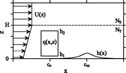
Figure 1 shows the schematic of a two-layer atmosphere considered in this study. The lower and upper layers represent the troposphere and stratosphere, respectively. The tropopause height is H. The stratospheric static stability N_S is larger than the tropospheric static stability N_T. The basic-state wind has a constant wind shear in the troposphere (U = U₀ + sz, where U₀ is the basic-state wind speed at the surface and s is the basic-state wind shear) and is constant in the stratosphere (U = U_H). Only positive U₀ and s are considered in this study. The convective forcing q represents the latent heat release from convective clouds and is specified as (5) $$q(x,z)=q_0\left\{\frac{a_{\mathrm{c}}^2}{{(x-c_{\mathrm{c}})}^2+a_{\mathrm{c}}^2}-\frac{a_{\mathrm{c}}{b}_{\mathrm{c}}}{{(x-c_{\mathrm{c}})}^2+b_{\mathrm{c}}^2}\right\},$$(5) where q₀ is the magnitude of the convective forcing, a_c is the half-width of the bell-shaped heating function, b_c is a constant (b_c > a_c), and c_c is the centre of the convective forcing in the x-direction. The convective forcing is present from z = h₁ to z = h₂, where h₁ and h₂ are the bottom and top heights of the convective forcing, respectively (Fig. 1). The mountain is specified by (6) $$h\left(x\right)=h_{\mathrm{m}}\frac{a_{\mathrm{m}}^2}{{(x-c_{\mathrm{m}})}^2+a_{\mathrm{m}}^2},$$(6) where h_m is the maximum height of the mountain, a_m is the half-width of the bell-shaped mountain function, and c_m is the centre of the mountain in the x-direction.

Fig. 1. Structure of a two-layer atmosphere in the presence of convective forcing and a mountain considered in this study.

Equations (1)–(4) can be combined into a single equation in the perturbation vertical velocity, which is Fourier-transformed (x → k) to obtain (7a) $$U^2{\widehat{w}}_{zz}+N^2\widehat{w}=\widehat{F},$$(7a) where (7b) $$\widehat{F}(k,z)=\frac{g{q}_0{a}_{\mathrm{c}}}{c_p{T}_0{N}_{\mathrm{T}}^2}(e^{-a_{\mathrm{c}}k}-e^{-b_{\mathrm{c}}k})e^{-ik{c}_{\mathrm{c}}}.$$(7b)

The general solutions of Eq. (7a(7a) $$U^2{\widehat{w}}_{zz}+N^2\widehat{w}=\widehat{F},$$(7a) ) for 0 ≤ z ≤ H and z > H are given, respectively, by (8a) $${\widehat{w}}_{\mathrm{T}}(k,z)=A{U}^{\frac{1}{2}+i\mu }+B{U}^{\frac{1}{2}-i\mu }+\widehat{F},$$(8a) (8b) $${\widehat{w}}_{\mathrm{S}}(k,z)=C{e}^{imz}+D{e}^{-imz}.$$(8b)

Here, μ = (Ri – 0.25)^1/2, where Ri (= N_T²/s²) is the tropospheric Richardson number, and m (= N_S/U_H) is the vertical wavenumber of the internal gravity wave in the stratosphere. By imposing bottom boundary condition [ŵ = ikU₀ĥ ≡ Ĝ; ĥ = h_ma_mexp{–k(a_m + ikc_m)}], upper radiation condition (D = 0 with U_H > 0), and interfacial boundary conditions (ŵ and ∂ŵ/∂z are continuous at z = h₁, h₂, and H), the analytic solutions in Fourier-transformed space for 0 ≤ z ≤ h₁, h₁ < z ≤ h₂, h₂ < z ≤ H, and z > H are obtained as, respectively, (9a) $$\begin{array}{c}{\widehat{w}}_1(k,z)=\widehat{G}\left(\frac{1-R{Z}_0^{-2i\mu }}{1-R}\right)Z_0^{\frac{1}{2}+i\mu }\\ -\widehat{F}\left(\frac{1-Z_0^{-2i\mu }}{1-R}\right)\left\{PR(Z_1^{\frac{1}{2}+i\mu }-Z_2^{\frac{1}{2}+i\mu })+Q{Z}_0^{2i\mu }(Z_1^{\frac{1}{2}-i\mu }-Z_2^{\frac{1}{2}-i\mu })\right\},\end{array}$$(9a) (9b) $${\widehat{w}}_2(k,z)={\widehat{w}}_1-\widehat{F}(P{Z}_1^{\frac{1}{2}+i\mu }+Q{Z}_1^{\frac{1}{2}-i\mu }-1),$$(9b) (9c) $${\widehat{w}}_3(k,z)={\widehat{w}}_1-\widehat{F}\left\{P(Z_1^{\frac{1}{2}+i\mu }-Z_2^{\frac{1}{2}+i\mu })+Q(Z_1^{\frac{1}{2}-i\mu }-Z_2^{\frac{1}{2}-i\mu })\right\},$$(9c) (9d) $${\widehat{w}}_4(k,z)=\left(\frac{1-R{Z}_{H0}^{-2i\mu }}{1-R}\right)\left[\widehat{G}{Z}_{H0}^{\frac{1}{2}+i\mu }-\widehat{F}\left\{P(Z_{H1}^{\frac{1}{2}+i\mu }-Z_{H2}^{\frac{1}{2}+i\mu })+Q{Z}_{H0}^{2i\mu }(Z_{H1}^{\frac{1}{2}-i\mu }-Z_{H2}^{\frac{1}{2}-i\mu })\right\}\right]e^{im\Delta z},$$(9d) where (9e) $$Z_i\hspace{0.17em}=\hspace{0.17em}\frac{U}{U_i},$$(9e) (9f) $$Z_{Hi}\hspace{0.17em}=\hspace{0.17em}\frac{U_H}{U_i},$$(9f) (9g) $$P\hspace{0.17em}=\hspace{0.17em}\frac{1}{2}+i\frac{1}{4\mu }$$(9g) (9h) $$Q\hspace{0.17em}=\hspace{0.17em}\frac{1}{2}-i\frac{1}{4\mu }$$(9h) (9i) $$R\hspace{0.17em}=\hspace{0.17em}\frac{\frac{1}{2}-i\left(\frac{N_{\mathrm{S}}}{N_{\mathrm{T}}}\sqrt{\text{Ri}}-\mu \right)}{\frac{1}{2}-i\left(\frac{N_{\mathrm{S}}}{N_{\mathrm{T}}}\sqrt{\text{Ri}}+\mu \right)}{Z}_{H0}^{2i\mu }$$(9i) (9j) $$\Delta z\hspace{0.17em}=\hspace{0.17em}z–H.$$(9j)

In Eqs. (9e)(9e) $$Z_i\hspace{0.17em}=\hspace{0.17em}\frac{U}{U_i},$$(9e) and (9f)(9f) $$Z_{Hi}\hspace{0.17em}=\hspace{0.17em}\frac{U_H}{U_i},$$(9f) , i = 0, 1, and 2 are for z = 0, h₁, and h₂, respectively.

Note that Eqs. (9a)–(9d) are linear combinations of orographically and convectively induced components. P(Q) represents the complex amplitude of upward (downward) propagating convectively forced internal gravity wave component generated at z = h₁ and h₂ (note that P and Q are a complex conjugate pair and P + Q = 1). R represents the complex reflection coefficient of the orographically/convectively forced internal gravity wave at the tropopause.

To get analytic solutions in physical space, we take the inverse Fourier transform (k → x) of Eqs. (9a)–(9d) and select the real parts of the transformed solutions. The orographically forced components of the solutions for 0 ≤ z ≤ H (j = 1, 2, and 3) and z > H are given, respectively, by (10a) $$\begin{array}{c}{w}_{j\mathrm{m}}(x,z)=Z_0^{\frac{1}{2}}[G_{\mathrm{R}}\left\{R_1\hspace{0.17em}\text{cos}\hspace{0.17em}({\theta }_1+{\theta }_{z0})-R_2\hspace{0.17em}\text{cos}\hspace{0.17em}({\theta }_2-{\theta }_{z0})\right\}\\ -G_{\mathrm{I}}\left\{R_1\hspace{0.17em}\text{sin}\hspace{0.17em}({\theta }_1+{\theta }_{z0})-R_2\hspace{0.17em}\text{sin}\hspace{0.17em}({\theta }_2-{\theta }_{z0})\right\}],\end{array}$$(10a) (10b) $$\begin{array}{c}{w}_{4\mathrm{m}}(x,z)=Z_{H0}^{\frac{1}{2}}[G_{\mathrm{R}}\left\{R_1\hspace{0.17em}\text{cos}\hspace{0.17em}({\theta }_1+{\theta }_{H0}+m\Delta z)-R_2\hspace{0.17em}\text{cos}\hspace{0.17em}({\theta }_2-{\theta }_{H0}+m\Delta z)\right\}\\ -G_{\mathrm{I}}\left\{R_1\hspace{0.17em}\text{sin}\hspace{0.17em}({\theta }_1+{\theta }_{H0}+m\Delta z)-R_2\hspace{0.17em}\text{sin}\hspace{0.17em}({\theta }_2-{\theta }_{H0}+m\Delta z)\right\}].\end{array}$$(10b)

The convectively forced components of the solutions for 0 ≤ z ≤ h₁, h₁ < z ≤ h₂, h₂ < z ≤ H, and z > H are given, respectively, by (11a) $$\begin{array}{c}{w}_{1\mathrm{c}}(x,z)=-\frac{N_{\mathrm{T}}}{2s\mu }[F_{\mathrm{R}}〈R_1[Z_1^{\frac{1}{2}}\left\{\hspace{0.17em}\text{cos}\hspace{0.17em}({\theta }_1+{\Theta }_{z1}^{+})-\hspace{0.17em}\text{cos}\hspace{0.17em}({\theta }_1-{\Theta }_{z1}^{-})\right\}\\ -Z_2^{\frac{1}{2}}\left\{\hspace{0.17em}\text{cos}\hspace{0.17em}({\theta }_1+{\Theta }_{z2}^{+})-\hspace{0.17em}\text{cos}\hspace{0.17em}({\theta }_1-{\Theta }_{z2}^{-})\right\}]\\ +R_2[Z_1^{\frac{1}{2}}\left\{\hspace{0.17em}\text{cos}\hspace{0.17em}({\theta }_2+{\Theta }_{z1}^{-})-\hspace{0.17em}\text{cos}\hspace{0.17em}({\theta }_2-{\Theta }_{z1}^{+})\right\}\\ -Z_2^{\frac{1}{2}}\left\{\hspace{0.17em}\text{cos}\hspace{0.17em}({\theta }_2+{\Theta }_{z2}^{-})-\hspace{0.17em}\text{cos}\hspace{0.17em}({\theta }_2-{\Theta }_{z2}^{+})\right\}]〉\\ -F_{\mathrm{I}}〈R_1[Z_1^{\frac{1}{2}}\left\{\hspace{0.17em}\text{sin}\hspace{0.17em}({\theta }_1+{\Theta }_{z1}^{+})-\hspace{0.17em}\text{sin}\hspace{0.17em}({\theta }_1-{\Theta }_{z1}^{-})\right\}\\ -Z_2^{\frac{1}{2}}\left\{\hspace{0.17em}\text{sin}\hspace{0.17em}({\theta }_1+{\Theta }_{z2}^{+})-\hspace{0.17em}\text{sin}\hspace{0.17em}({\theta }_1-{\Theta }_{z2}^{-})\right\}]\\ +R_2[Z_1^{\frac{1}{2}}\left\{\hspace{0.17em}\text{sin}\hspace{0.17em}({\theta }_2+{\Theta }_{z1}^{-})-\hspace{0.17em}\text{sin}\hspace{0.17em}({\theta }_2-{\Theta }_{z1}^{+})\right\}\\ -Z_2^{\frac{1}{2}}\left\{\hspace{0.17em}\text{sin}\hspace{0.17em}({\theta }_2+{\Theta }_{z2}^{-})-\hspace{0.17em}\text{sin}\hspace{0.17em}({\theta }_2-{\Theta }_{z2}^{+})\right\}]〉],\end{array}$$(11a) (11b) $$w_{2\mathrm{c}}(x,z)=w_{1\mathrm{c}}-\left(\frac{N_{\mathrm{T}}{F}_{\mathrm{R}}}{s\mu }{Z}_1^{\frac{1}{2}}\hspace{0.17em}\text{cos}\hspace{0.17em}{\Theta }_{z1}^{-}-F_{\mathrm{R}}\right),$$(11b) (11c) $$w_{3\mathrm{c}}(x,z)=w_{1\mathrm{c}}-\frac{N_{\mathrm{T}}{F}_{\mathrm{R}}}{s\mu }\left(Z_1^{\frac{1}{2}}\hspace{0.17em}\text{cos}\hspace{0.17em}{\Theta }_{z1}^{-}-Z_2^{\frac{1}{2}}\hspace{0.17em}\text{cos}\hspace{0.17em}{\Theta }_{z2}^{-}\right),$$(11c) (11d) $$\begin{array}{c}{w}_{4\mathrm{c}}(x,z)=-\frac{N_{\mathrm{T}}}{s\mu }[F_{\mathrm{R}}\left\{R_1\hspace{0.17em}\text{cos}\hspace{0.17em}\left({\theta }_1+{\theta }_{H0}+m\Delta z\right)-R_2\hspace{0.17em}\text{cos}\hspace{0.17em}\left({\theta }_2-{\theta }_{H0}+m\Delta z\right)\right\}\\ -F_{\mathrm{I}}\left\{R_1\hspace{0.17em}\text{sin}\hspace{0.17em}\left({\theta }_1+{\theta }_{H0}+m\Delta z\right)-R_2\hspace{0.17em}\text{sin}\hspace{0.17em}\left({\theta }_2-{\theta }_{H0}+m\Delta z\right)\right\}]\times \\ \left\{Z_{H1}^{\frac{1}{2}}\hspace{0.17em}\text{cos}\hspace{0.17em}\left({\theta }_{10}-{\hspace{0.17em}\text{tan}\hspace{0.17em}}^{-1}\frac{1}{2\mu }\right)-Z_{H2}^{\frac{1}{2}}\hspace{0.17em}\text{cos}\hspace{0.17em}\left({\theta }_{20}-{\hspace{0.17em}\text{tan}\hspace{0.17em}}^{-1}\frac{1}{2\mu }\right)\right\}.\end{array}$$(11d)

In Eqs. (10) and (11), (12a) $$G_{\mathrm{R}}+i{G}_{\mathrm{I}}=-h_{\mathrm{m}}{a}_{\mathrm{m}}{U}_0\frac{2a_{\mathrm{m}}(x-c_{\mathrm{m}})+i\{{(x-c_{\mathrm{m}})}^2-a_{\mathrm{m}}^2\}}{{(x-c_{\mathrm{m}})}^2+a_{\mathrm{m}}^2}$$(12a) (12b) $$F_{\mathrm{R}}+i{F}_{\mathrm{I}}=\frac{q_{0}g{a}_{\mathrm{c}}}{c_p{T}_0{N}_{\mathrm{T}}^2}\left\{\frac{a_{\mathrm{c}}+i(x-c_{\mathrm{c}})}{{(x-c_{\mathrm{c}})}^2+a_{\mathrm{c}}^2}-\frac{b_{\mathrm{c}}+(x-c_{\mathrm{c}})}{{(x-c_{\mathrm{c}})}^2+b_{\mathrm{c}}^2}\right\}$$(12b) (12c) $$\frac{1}{1-R}\equiv R_1{\mathrm{e}}^{i{\theta }_1},$$(12c) (12d) $$\frac{R}{1-R}\equiv R_2{\mathrm{e}}^{i{\theta }_2},$$(12d) (12e) $${\theta }_{zl}=\mu \hspace{0.17em}\text{ln}\hspace{0.17em}\frac{U}{U_l},$$(12e) (12f) $${\theta }_{pq}=\mu \hspace{0.17em}\text{ln}\hspace{0.17em}\frac{U_p}{U_q},$$(12f) (12g) $${\Theta }_{zj}^{\pm }={\theta }_{z0}\pm \left({\theta }_{j0}-{\hspace{0.17em}\text{tan}\hspace{0.17em}}^{-1}\frac{1}{2\mu }\right)$$(12g)

In Eq. (12(12a) $$G_{\mathrm{R}}+i{G}_{\mathrm{I}}=-h_{\mathrm{m}}{a}_{\mathrm{m}}{U}_0\frac{2a_{\mathrm{m}}(x-c_{\mathrm{m}})+i\{{(x-c_{\mathrm{m}})}^2-a_{\mathrm{m}}^2\}}{{(x-c_{\mathrm{m}})}^2+a_{\mathrm{m}}^2}$$(12a) e), l = 0, 1, and 2 are for z = 0, h₁, and h₂, respectively. In Eq. (12(12a) $$G_{\mathrm{R}}+i{G}_{\mathrm{I}}=-h_{\mathrm{m}}{a}_{\mathrm{m}}{U}_0\frac{2a_{\mathrm{m}}(x-c_{\mathrm{m}})+i\{{(x-c_{\mathrm{m}})}^2-a_{\mathrm{m}}^2\}}{{(x-c_{\mathrm{m}})}^2+a_{\mathrm{m}}^2}$$(12a) f), p and q = 0, 1, 2, and H are for z = 0, h₁, h₂, and H, respectively. In Eq. (12(12a) $$G_{\mathrm{R}}+i{G}_{\mathrm{I}}=-h_{\mathrm{m}}{a}_{\mathrm{m}}{U}_0\frac{2a_{\mathrm{m}}(x-c_{\mathrm{m}})+i\{{(x-c_{\mathrm{m}})}^2-a_{\mathrm{m}}^2\}}{{(x-c_{\mathrm{m}})}^2+a_{\mathrm{m}}^2}$$(12a) g), j = 1 and 2 are for z = h₁ and h₂, respectively.

We consider the finite-depth convective forcing which extends from z = h₁ = 1 km to z = h₂ = 11 km vertically and has the half-width of heating a_c = 10 km and b_c = 5a_c. The centre of the bell-shaped mountain is c_m = 0 km with a_m = 10 km. The tropospheric buoyancy frequency is specified as N_T = 0.01 s⁻¹, the basic-state wind speed at the surface as U₀ = 10 m s⁻¹, and the tropopause height as H = 12 km. The stratospheric buoyancy frequency N_S, the basic-state wind speed in the stratosphere U_H, and the centre of the convective forcing c_c are different in each case. We name each case NxUyy in which N_S = 0.0x s⁻¹ and U_H = yy m s⁻¹ are used. The basic-state wind shear s is determined by U₀, U_H, and H, and the tropospheric Richardson number Ri by N_T, U₀, U_H, and H. The reference temperature is specified as T₀ = 273.15 K. The maximum height of the mountain h_m = 500 m and the magnitude of the convective forcing q₀ = 1 J kg⁻¹ s⁻¹ are adapted from Smith and Lin (1982) and Chun and Baik (1998, 2002), respectively, in which orographically and convectively forced mesoscale flows and momentum fluxes are discussed.

3. Results and discussion

3.1. Orographic–convective flows

The flows forced by each forcing are first presented before examining the linear interaction between orographic and convective flows. In reality, wind shear exists in the troposphere and the static stability in the troposphere is different from that in the stratosphere. In this study, however, the cases without wind shear or stability jump are also considered to isolate wind shear or stability jump effects. The flows computed for such cases exhibit well-known features of orographically or convectively forced flows. Fig. 2 shows orographically and convectively forced perturbation vertical velocity fields in the cases of N1U10, N1U20, and N2U10 with c_m = 0 km and c_c = 0 km. The effects of tropospheric wind shear on orographically/convectively forced flow can be examined by comparing the N1U10 and N1U20 cases. The effects of static stability difference between the troposphere and the stratosphere on orographically/convectively forced flow can be examined by comparing the N1U10 and N2U10 cases. Under the no-slip boundary condition at the surface, upward and downward flows are orographically generated on the upslope and downslope of the mountain, respectively (Fig. 2a–c). Internal gravity waves are generated in the stably stratified atmosphere, and the perturbation vertical velocity fields exhibit a wavy structure in the vertical direction (Queney, 1948; Durran, 1992). The alternating pattern of the perturbation vertical velocity according to internal gravity waves generated at the surface is clearly seen in the entire atmosphere. The convection forces a deep upward motion near the convective forcing centre given a small thermal Froude number (Lin, 2007) and a low-level compensating downward motion upstream of the convection (Fig. 2d–f). These are well-known characteristics of convectively forced flows (Lin and Smith, 1986; Han and Baik, 2009). Above the convection top, the alternating pattern of the perturbation vertical velocity according to internal gravity waves clearly appears. Without the basic-state wind shear, the vertical wavelength of the internal gravity wave in the troposphere is 2πU₀/N_T = 6.28 km (the cases N1U10 and N2U10) as reported in many previous studies (Han and Baik, 2009).

Fig. 2. (a)–(c) Orographically and (d)–(f) convectively forced perturbation vertical velocity fields in the cases of N1U10 for (a) and (d), N1U20 for (b) and (e), and N2U10 for (c) and (f) with c_m = 0 km and c_c = 0 km. The rectangle in (d)–(f) represents the concentrated convective forcing region. The contour line information (unit: m s⁻¹) is given at the bottom of each panel.

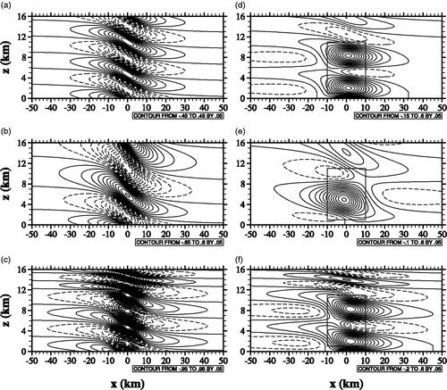
In the case with wind shear, the increase of the basic-state wind speed with height strengthens the orographically forced perturbation vertical velocity (Fig. 2b). The vertical wavelength of the internal gravity wave is longer in the case with wind shear than in the cases without wind shear due to the vertically increasing basic-state wind speed. The wavy structure of the convectively forced vertical velocity field in the troposphere is less prominent in the case with wind shear (Fig. 2e). The main updraft is more concentrated and has a single-cell structure in the region of concentrated convective forcing. However, the compensating downward motion is weaker in the case with wind shear (Fig. 2e) compared to the cases without wind shear (Fig. 2d and f). See the contour line in the region of compensating downward motion and the contour line information at the bottom of each panel (Fig. 2d–f). Compared to the cases without wind shear, the compensating downward motion is located closer to the convection centre. In the cases without wind shear, on the upstream side, orographically forced waves are out of phase with convectively forced waves by ∼180° (compare Fig. 2a and d and also compare Fig. 2c and f). For this reason, flows forced by convection over the mountain peak would be negatively combined with orographically forced flows on the upstream side. In the case with wind shear, the convectively forced single-cell shaped main upward motion would be positively (negatively) combined with the updraft (downdraft) near the convection centre above the mountain peak (Fig. 2b and e).

In the case with stability jump (N2U10), the vertical wavelength of the internal gravity wave in the stratosphere is shorter than that in the case without stability jump (N1U10) due to the higher stratospheric buoyancy frequency (Fig. 2c and f). The main structure of the perturbation vertical velocity field in the troposphere is similar to that in the case without stability jump. However, the induced flows are stronger in the case of N2U10 than in the case of N1U10. The wave reflection at the tropopause plays a role in strengthening the flows. The analysis of the wave reflection is provided in Section 3.2.

This study considers a linear, hydrostatic system. Therefore, we need to choose the values of the basic-state wind speed and static stability, the maximum height and half-width of the mountain, and the magnitude and half-width of the convective forcing so that the linear, hydrostatic approximations are valid (Fig. 2). The Froude number, defined as Fr = U₀/(N_Th_m), is a measure of non-linearity of orographically forced internal gravity waves (the larger the more linear). Non-linearity of thermally forced internal gravity waves can be measured by μ_NL = (gq₀a_c)/(c_pT₀N_TU₀²) (Lin and Chun, 1991; Chun and Baik, 1994) (the smaller the more linear). For the uniform basic-state flow, the calculated values of Fr and μ_NL are 2 and 0.36, respectively. For the shear flow, if the vertically averaged basic-state wind speed in the troposphere is used, Fr =3 and μ_NL = 0.16. These values of Fr and μ_NL indicate that the flow system becomes linear (Lin, 2007). Non-hydrostaticity of thermally forced internal gravity waves can be measured by β = U₀/(N_Ta_c) (Woo et al., 2013) (the smaller the more hydrostatic). The calculated value of β is 0.1 for the uniform basic-sate flow. For the shear flow, if the basic-state wind speed averaged over the troposphere is used, the calculated value of β is 0.15. These values of β imply that the flow system becomes hydrostatic (Woo et al., 2013). The parameter U₀/(N_Ta_m) is a measure of non-hydrostaticity of orographically forced internal gravity waves (Lin, 2007). A similar analysis shows that the flow system becomes hydrostatic.

For the linear and hydrostatic approximations to be valid, μ_NL ≪ 1, Fr ≫ 1, and β ≪ ∼0.3 [non-hydrostatic feature appears when β = 0.3 in Woo et al. (2013)] should be satisfied. If Fr ≪ 1 (large h_m and N_T or small U₀), μ_NL ≫ 1 (large q₀ or small N_T and U₀), or β ≫ ∼0.3 (large U₀ or small N_T and a_c/m), the linear assumption for the orographically forced flows, the linear assumption for the convectively forced flows, or the hydrostatic assumption for both the orographically and convectively forced flows, respectively, is not valid. Typical characteristics of orographically and convectively forced mesoscale flows and gravity waves in non-linear or non-hydrostatic systems can be found in Lin (2007).

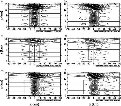
The convectively forced vertical flows are examined. In all cases (N1U10, N1U20, N2U10, and N2U20), the convectively forced main upward motion is located over the upslope of the mountain. See Fig. 2d–f that shows the convectively forced perturbation vertical velocity fields in the cases of N1U10, N1U20, and N2U10. Note that the case of N2U20 is not shown in Fig. 2. The convectively forced main upward motion is positively combined with orographically forced updrafts in the convection layer. Fig. 3 shows perturbation vertical velocity fields with the centre of the convective forcing on the upstream of the mountain (c_c = –10 km), where the orographically forced upward/downward motion over the upslope of the mountain is significant. As a result, a deep layer of strong updraft appears aloft upstream of the mountain (Fig. 3a and c). The main internal gravity wave bands generated by both forcings are concentrated slightly downstream of the mountain centre (Fig. 3a and c). In the cases with wind shear, the convectively forced upward motion creates an even deeper layer of strong updraft upslope of the mountain compared to the cases without wind shear (compare Fig. 3a and b and also Fig. 3c and d). With the low-level upslope wind, however, the positive combination of the convectively forced upward motion is weaker in the cases with wind shear than in the cases without wind shear. The mountain waves are stronger and more concentrated over the mountain centre in the cases with wind shear than in the cases without wind shear. The strong downdraft area of the mountain waves in the lower convection layer is broader in the cases with wind shear than in the cases without wind shear. As in Fig. 2, the flows forced by both forcings are stronger in the cases with stability jump due to the wave reflection at the tropopause than in the cases with uniform stability in the entire atmosphere (compare Fig. 3a and c and also Fig. 3b and d).

Fig. 3. Perturbation vertical velocity fields in the cases of (a) N1U10, (b) N1U20, (c) N2U10, and (d) N2U20 with c_c = –10 km. The rectangle in the troposphere represents the concentrated convective forcing region. The contour line information (unit: m s⁻¹) is given at the bottom of each panel.

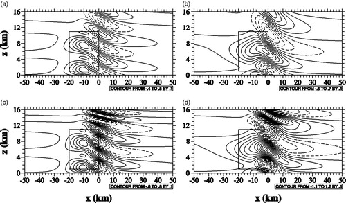
Observations indicate that orographic uplift in the upslope region of a mountain can produce precipitating deep convective clouds when the atmosphere is conditionally unstable (Houze, 2014). The convective clouds produced by the orographic uplift can be further enhanced by the low-level updraft forced by the mountain in the upslope region. This is dynamically implied in Fig. 3.

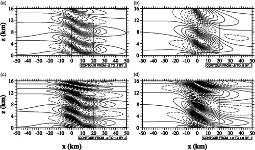
The cases with the convective forcing on the lee side of the mountain, where the orographically forced upward/downward motion of the downslope of the mountain is significant, are considered. In this situation, it may be supposed that the convective forcing results from some forcing other than the mountain. In the convection layer over the downslope of the mountain, the convectively forced upward motion positively interacts with the updrafts of mountain waves. In the cases without stability jump, the maximum amplitude of resultant waves appears above the downslope of the mountain as a result of the positive combination of orographically forced flows with convectively forced flows there (Fig. 4a and b). In the cases with stability jump, the maximum amplitude of the strengthened resultant waves over the mountain is located over the mountain peak (Fig. 4c and d).

Fig. 4. The same as Fig. 3 except for c_c = 10 km.

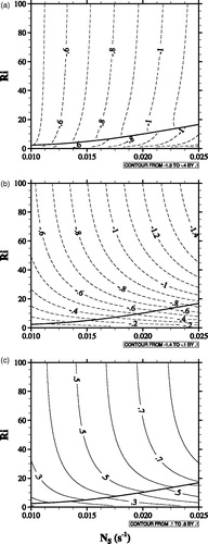
Forced uplift of a moist air over the upslope of a mountain occasionally produces orographic clouds and precipitation. The horizontal and vertical motion forced by various factors, such as latent heat and local circulation, enhances or suppresses orographically forced uplift. To examine the effects of convectively forced vertical motion on orographically forced vertical motion on the upslope of the mountain, we calculate the ratio of the convectively forced perturbation vertical velocity to the orographically forced perturbation vertical velocity at (x, z) = (c_m – a_m, h₁). Note that c_m – a_m = –10 km and h₁ = 1 km. The results are in Fig. 5. The ratio is calculated as a function of c_c and U_H (Fig. 5a and b) and as a function of c_c and N_S (Fig. 5c and d). In Fig. 5 (and also in Figs. 6, 7, and 9), U₀ = 10 m s⁻¹, U_H = 10–50 m s⁻¹, N_T = 0.01 s⁻¹, and N_S = 0.01–0.025 s⁻¹ are considered. These ranges sufficiently cover the typical wind speed in the troposphere [see Holton and Hakim (2012)] and the static stability in the stratosphere [see Fueglistaler et al. (2011)].

Fig. 5. Fields of the ratio of the convectively forced perturbation vertical velocity to the orographically forced perturbation vertical velocity at (x, z) = (c_m – a_m, h₁) as a function of c_c and U_H in the cases of (a) N1Uyy and (b) N2Uyy and as a function of c_c and N_S in the cases of (c) NxU10 and (d) NxU20.

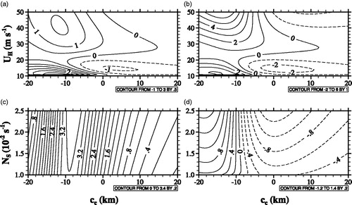
Fig. 6. (a) R₀, (b) R₁, (c) R₂, (d) θ₀, (e) θ₁, and (f) θ₂ as a function of the stratospheric buoyancy frequency and the Richardson number. The values of θ₀, θ₁, and θ₂ are in radian.

When the convection centre is located at c_c ≲ –10 km, the convectively forced upward motion is positively combined with the orographic uplift. For weak wind shear (s ≲ 8.3 × 10⁻⁴s⁻¹; U_H ≲ 20 m s⁻¹), the positive combination is stronger as wind shear becomes weaker (Fig. 5a and b). For strong wind shear, the convectively forced flows tend to be positively (negatively) combined with the orographic uplift when the convection centre is located upstream (downstream) of the mountain, and how strong the combination is depends on the wind shear. When the convection centre is located at c_c ≳ 0 km, the convectively forced compensating downward motion is generally negatively combined with the orographic uplift. Depending on the location of the boundary between the convectively forced upward motion and the compensating downward motion, the ratio has different signs. For this reason, there is a range of wind shear in which the ratio is positive (negative), although the convective forcing is located above the lee (upstream) side of the mountain.

The positive (negative) combination of the convectively forced upward motion (compensating downward motion) with the orographic uplift is strong in the case with large stability jump except when there is weak or no wind shear with c_c ≲ –10 km (Fig. 5). Without wind shear, the convection forces upward motion at (x, z) = (c_m – a_m, h₁) in a wide range of c_c and N_S because the compensating downward motion is located far upstream of the convection centre. The positive interaction is strongest when the convection centre is located at x ∼ –9 km (Fig. 5c). When wind shear exists, however, the main upward motion (compensating downward motion) is positively (negatively) combined with the orographic uplift and the level of the interaction is stronger with larger stability jump (Fig. 5d).

3.2. Gravity-wave reflection

As mentioned in Section 3.1, the stability jump at the tropopause causes the reflection of the orographically/convectively forced internal gravity waves, and the reflected waves affect flows in both the troposphere and the stratosphere. The complex reflection coefficient R at the tropopause is given in Eq. (9(9a) $$\begin{array}{c}{\widehat{w}}_1(k,z)=\widehat{G}\left(\frac{1-R{Z}_0^{-2i\mu }}{1-R}\right)Z_0^{\frac{1}{2}+i\mu }\\ -\widehat{F}\left(\frac{1-Z_0^{-2i\mu }}{1-R}\right)\left\{PR(Z_1^{\frac{1}{2}+i\mu }-Z_2^{\frac{1}{2}+i\mu })+Q{Z}_0^{2i\mu }(Z_1^{\frac{1}{2}-i\mu }-Z_2^{\frac{1}{2}-i\mu })\right\},\end{array}$$(9a) i). The complex reflection coefficient R [≡ R₀exp(iθ₀), where R₀ is the reflectivity at the tropopause and θ₀ is the phase shift angle] can be rewritten as (13) $$R=\sqrt{\frac{\frac{1}{4}+{\left(\frac{N_{\mathrm{S}}}{N_{\mathrm{T}}}\sqrt{\text{Ri}}-\mu \right)}^2}{\frac{1}{4}+{\left(\frac{N_{\mathrm{S}}}{N_{\mathrm{T}}}\sqrt{\text{Ri}}+\mu \right)}^2}}\hspace{0.17em}\text{exp}\hspace{0.17em}\left\{i{\hspace{0.17em}\text{tan}\hspace{0.17em}}^{-1}\frac{\mu \left(1+2\hspace{0.17em}\text{ln}\hspace{0.17em}{Z}_{H0}\right)}{\frac{1}{4}+\left(\frac{N_{\mathrm{S}}}{N_{\mathrm{T}}}\sqrt{\text{Ri}}-{\mu }^2\right)}\right\}.$$(13)

The orographically forced internal gravity waves propagate upward from the surface. At the tropopause, the waves are partially reflected due to the discontinuity of the static stability between the troposphere and the stratosphere. The partially reflected waves at the tropopause are totally reflected at the surface and propagate upward again. To account for infinite reflections in this way, the upward propagating wave component is multiplied by 1/(1–R) and the downward propagating wave component is multiplied by R/(1–R) [see Eqs. (9i)(9i) $$R\hspace{0.17em}=\hspace{0.17em}\frac{\frac{1}{2}-i\left(\frac{N_{\mathrm{S}}}{N_{\mathrm{T}}}\sqrt{\text{Ri}}-\mu \right)}{\frac{1}{2}-i\left(\frac{N_{\mathrm{S}}}{N_{\mathrm{T}}}\sqrt{\text{Ri}}+\mu \right)}{Z}_{H0}^{2i\mu }$$(9i) , (12c)(12c) $$\frac{1}{1-R}\equiv R_1{\mathrm{e}}^{i{\theta }_1},$$(12c) , and (12d)(12d) $$\frac{R}{1-R}\equiv R_2{\mathrm{e}}^{i{\theta }_2},$$(12d) ]. The convectively forced internal gravity waves that originate from z = h₁ and h₂ propagate upward and downward with fractions of P and Q, respectively. Depending on the convection bottom/top heights and tropopause height, upward and downward propagating wave components are multiplied by 1/(1–R) and R/(1–R), respectively, so that (14a) $$\frac{1}{1-R}=\frac{1}{\sqrt{{\left(1-R_0\hspace{0.17em}\text{cos}\hspace{0.17em}{\theta }_0\right)}^2+R_0^2{\hspace{0.17em}\text{sin}\hspace{0.17em}}^2{\theta }_0}}\text{exp}\hspace{0.17em}\left\{i{\hspace{0.17em}\text{tan}\hspace{0.17em}}^{-1}\frac{R_0\hspace{0.17em}\text{sin}\hspace{0.17em}{\theta }_0}{1-R_0\hspace{0.17em}\text{cos}\hspace{0.17em}{\theta }_0}\right\},$$(14a) (14b) $$\frac{R}{1-R}=\frac{R_0}{\sqrt{{\left(\hspace{0.17em}\text{cos}\hspace{0.17em}{\theta }_0-R_0\right)}^2+{\hspace{0.17em}\text{sin}\hspace{0.17em}}^2{\theta }_0}}\text{exp}\hspace{0.17em}\left\{i{\hspace{0.17em}\text{tan}\hspace{0.17em}}^{-1}\frac{\hspace{0.17em}\text{sin}\hspace{0.17em}{\theta }_0}{\hspace{0.17em}\text{cos}\hspace{0.17em}{\theta }_0-R_0}\right\}.$$(14b)

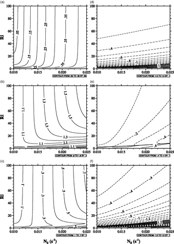
Fig. 6 shows R₀, R₁, R₂, θ₀, θ₁, and θ₂ as functions of the stratospheric buoyancy frequency and the Richardson number. For a given N_S, the reflectivity R₀ decreases as Ri increases. For a given N_S, R₀ is very sensitive to Ri when Ri is very small. For a given Ri, R₀ increases with increasing N_S. When Ri is large, R₀ tends to be independent of Ri for a given N_S and converges to (15) $$R_0\approx \frac{N_{\mathrm{S}}-N_{\mathrm{T}}}{N_{\mathrm{S}}+N_{\mathrm{T}}}.$$(15)

Note that R₀ in Eqs. (13)(13) $$R=\sqrt{\frac{\frac{1}{4}+{\left(\frac{N_{\mathrm{S}}}{N_{\mathrm{T}}}\sqrt{\text{Ri}}-\mu \right)}^2}{\frac{1}{4}+{\left(\frac{N_{\mathrm{S}}}{N_{\mathrm{T}}}\sqrt{\text{Ri}}+\mu \right)}^2}}\hspace{0.17em}\text{exp}\hspace{0.17em}\left\{i{\hspace{0.17em}\text{tan}\hspace{0.17em}}^{-1}\frac{\mu \left(1+2\hspace{0.17em}\text{ln}\hspace{0.17em}{Z}_{H0}\right)}{\frac{1}{4}+\left(\frac{N_{\mathrm{S}}}{N_{\mathrm{T}}}\sqrt{\text{Ri}}-{\mu }^2\right)}\right\}.$$(13) and (15)(15) $$R_0\approx \frac{N_{\mathrm{S}}-N_{\mathrm{T}}}{N_{\mathrm{S}}+N_{\mathrm{T}}}.$$(15) are always less than 1. The phase shift angle θ₀ (–π/2 ≤ θ₀ ≤ π/2) is negative for large Ri. For very small Ri, the sign of θ₀ is changed to positive. This sudden phase reversal occurs when Ri = [{N_S + (N_S² + 2N_T²)^1/2}/2N_T]². R₁ and R₂ are small when N_S and Ri are close to the boundary where the phase reversal of θ₀ occurs. For large Ri, both R₁ and R₂ increase with increasing N_S. For this reason, as stated above, the resultant wave strengths are stronger in the presence of stability jump. The phase shift angles θ₁ and θ₂ are negative for large Ri. The magnitudes of both phase shift angles are smaller for larger Ri (weaker wind shear) and are increased with increasing N_S for a given large Ri. Both phase shift angles change the sign in a manner similar to θ₀. The phase shift angle θ₂ has an additional sudden phase reversal when R₀ = cosθ₀. For a given N_S, the dependency of θ₂ on Ri is stronger than that of θ₁.

The analytic solutions for the orographically forced perturbation vertical velocity for 0 ≤ z ≤ H [Eq. (10(10a) $$\begin{array}{c}{w}_{j\mathrm{m}}(x,z)=Z_0^{\frac{1}{2}}[G_{\mathrm{R}}\left\{R_1\hspace{0.17em}\text{cos}\hspace{0.17em}({\theta }_1+{\theta }_{z0})-R_2\hspace{0.17em}\text{cos}\hspace{0.17em}({\theta }_2-{\theta }_{z0})\right\}\\ -G_{\mathrm{I}}\left\{R_1\hspace{0.17em}\text{sin}\hspace{0.17em}({\theta }_1+{\theta }_{z0})-R_2\hspace{0.17em}\text{sin}\hspace{0.17em}({\theta }_2-{\theta }_{z0})\right\}],\end{array}$$(10a) a)] at the mountain centre and the convectively forced perturbation vertical velocity for 0 ≤ z ≤ h₁ [Eq. (11(11a) $$\begin{array}{c}{w}_{1\mathrm{c}}(x,z)=-\frac{N_{\mathrm{T}}}{2s\mu }[F_{\mathrm{R}}〈R_1[Z_1^{\frac{1}{2}}\left\{\hspace{0.17em}\text{cos}\hspace{0.17em}({\theta }_1+{\Theta }_{z1}^{+})-\hspace{0.17em}\text{cos}\hspace{0.17em}({\theta }_1-{\Theta }_{z1}^{-})\right\}\\ -Z_2^{\frac{1}{2}}\left\{\hspace{0.17em}\text{cos}\hspace{0.17em}({\theta }_1+{\Theta }_{z2}^{+})-\hspace{0.17em}\text{cos}\hspace{0.17em}({\theta }_1-{\Theta }_{z2}^{-})\right\}]\\ +R_2[Z_1^{\frac{1}{2}}\left\{\hspace{0.17em}\text{cos}\hspace{0.17em}({\theta }_2+{\Theta }_{z1}^{-})-\hspace{0.17em}\text{cos}\hspace{0.17em}({\theta }_2-{\Theta }_{z1}^{+})\right\}\\ -Z_2^{\frac{1}{2}}\left\{\hspace{0.17em}\text{cos}\hspace{0.17em}({\theta }_2+{\Theta }_{z2}^{-})-\hspace{0.17em}\text{cos}\hspace{0.17em}({\theta }_2-{\Theta }_{z2}^{+})\right\}]〉\\ -F_{\mathrm{I}}〈R_1[Z_1^{\frac{1}{2}}\left\{\hspace{0.17em}\text{sin}\hspace{0.17em}({\theta }_1+{\Theta }_{z1}^{+})-\hspace{0.17em}\text{sin}\hspace{0.17em}({\theta }_1-{\Theta }_{z1}^{-})\right\}\\ -Z_2^{\frac{1}{2}}\left\{\hspace{0.17em}\text{sin}\hspace{0.17em}({\theta }_1+{\Theta }_{z2}^{+})-\hspace{0.17em}\text{sin}\hspace{0.17em}({\theta }_1-{\Theta }_{z2}^{-})\right\}]\\ +R_2[Z_1^{\frac{1}{2}}\left\{\hspace{0.17em}\text{sin}\hspace{0.17em}({\theta }_2+{\Theta }_{z1}^{-})-\hspace{0.17em}\text{sin}\hspace{0.17em}({\theta }_2-{\Theta }_{z1}^{+})\right\}\\ -Z_2^{\frac{1}{2}}\left\{\hspace{0.17em}\text{sin}\hspace{0.17em}({\theta }_2+{\Theta }_{z2}^{-})-\hspace{0.17em}\text{sin}\hspace{0.17em}({\theta }_2-{\Theta }_{z2}^{+})\right\}]〉],\end{array}$$(11a) a)] at the convection centre can be written as, respectively, (16a) $$w_{\mathrm{m}}\left(z\right)=-G_{\mathrm{I}}{}_{(x=0)}{Z}_0^{\frac{1}{2}}\left\{\hspace{0.17em}\text{cos}\hspace{0.17em}{\theta }_{z0}(R_1\hspace{0.17em}\text{sin}\hspace{0.17em}{\theta }_1-R_2\hspace{0.17em}\text{sin}\hspace{0.17em}{\theta }_2)+\hspace{0.17em}\text{sin}\hspace{0.17em}{\theta }_{z0}(R_1\hspace{0.17em}\text{cos}\hspace{0.17em}{\theta }_1+R_2\hspace{0.17em}\text{cos}\hspace{0.17em}{\theta }_2)\right\},$$(16a) (16b) $$\begin{array}{c}{w}_{\mathrm{c}}\left(z\right)=-F_{\mathrm{R}}{}_{(x=0)}\frac{N_{\mathrm{T}}}{s\mu }\text{sin}\hspace{0.17em}{\theta }_{z0}\left(Z_1^{\frac{1}{2}}-Z_2^{\frac{1}{2}}\right)\{\hspace{0.17em}\text{cos}\hspace{0.17em}\left({\theta }_{z0}-{\hspace{0.17em}\text{tan}\hspace{0.17em}}^{-1}\frac{1}{2\mu }\right)(R_1\hspace{0.17em}\text{sin}\hspace{0.17em}{\theta }_1-R_2\hspace{0.17em}\text{sin}\hspace{0.17em}{\theta }_2)\\ +\hspace{0.17em}\text{sin}\hspace{0.17em}\left({\theta }_{z0}-{\hspace{0.17em}\text{tan}\hspace{0.17em}}^{-1}\frac{1}{2\mu }\right)(R_1\hspace{0.17em}\text{cos}\hspace{0.17em}{\theta }_1-R_2\hspace{0.17em}\text{cos}\hspace{0.17em}{\theta }_2)\}.\end{array}$$(16b)

Because the second terms on the right hand sides of Eqs. (11b)(11b) $$w_{2\mathrm{c}}(x,z)=w_{1\mathrm{c}}-\left(\frac{N_{\mathrm{T}}{F}_{\mathrm{R}}}{s\mu }{Z}_1^{\frac{1}{2}}\hspace{0.17em}\text{cos}\hspace{0.17em}{\Theta }_{z1}^{-}-F_{\mathrm{R}}\right),$$(11b) and (11c)(11c) $$w_{3\mathrm{c}}(x,z)=w_{1\mathrm{c}}-\frac{N_{\mathrm{T}}{F}_{\mathrm{R}}}{s\mu }\left(Z_1^{\frac{1}{2}}\hspace{0.17em}\text{cos}\hspace{0.17em}{\Theta }_{z1}^{-}-Z_2^{\frac{1}{2}}\hspace{0.17em}\text{cos}\hspace{0.17em}{\Theta }_{z2}^{-}\right),$$(11c) do not depend on the stratospheric buoyancy frequency, the terms in braces in Eqs. (16a)(16a) $$w_{\mathrm{m}}\left(z\right)=-G_{\mathrm{I}}{}_{(x=0)}{Z}_0^{\frac{1}{2}}\left\{\hspace{0.17em}\text{cos}\hspace{0.17em}{\theta }_{z0}(R_1\hspace{0.17em}\text{sin}\hspace{0.17em}{\theta }_1-R_2\hspace{0.17em}\text{sin}\hspace{0.17em}{\theta }_2)+\hspace{0.17em}\text{sin}\hspace{0.17em}{\theta }_{z0}(R_1\hspace{0.17em}\text{cos}\hspace{0.17em}{\theta }_1+R_2\hspace{0.17em}\text{cos}\hspace{0.17em}{\theta }_2)\right\},$$(16a) and (16b)(16b) $$\begin{array}{c}{w}_{\mathrm{c}}\left(z\right)=-F_{\mathrm{R}}{}_{(x=0)}\frac{N_{\mathrm{T}}}{s\mu }\text{sin}\hspace{0.17em}{\theta }_{z0}\left(Z_1^{\frac{1}{2}}-Z_2^{\frac{1}{2}}\right)\{\hspace{0.17em}\text{cos}\hspace{0.17em}\left({\theta }_{z0}-{\hspace{0.17em}\text{tan}\hspace{0.17em}}^{-1}\frac{1}{2\mu }\right)(R_1\hspace{0.17em}\text{sin}\hspace{0.17em}{\theta }_1-R_2\hspace{0.17em}\text{sin}\hspace{0.17em}{\theta }_2)\\ +\hspace{0.17em}\text{sin}\hspace{0.17em}\left({\theta }_{z0}-{\hspace{0.17em}\text{tan}\hspace{0.17em}}^{-1}\frac{1}{2\mu }\right)(R_1\hspace{0.17em}\text{cos}\hspace{0.17em}{\theta }_1-R_2\hspace{0.17em}\text{cos}\hspace{0.17em}{\theta }_2)\}.\end{array}$$(16b) determine the characteristics of the waves in the troposphere affected by the wave reflection at the tropopause.

The surface vertical velocity at the centre of each forcing is zero and the vertically varying pattern of the vertical velocity at the centre of each forcing is like a sine function rather than a cosine function (Fig. 2), and our calculation indicates that R₁sinθ₁ – R₂sinθ₂ is almost zero. Accordingly, among the two terms in braces in Eq. (16(16a) $$w_{\mathrm{m}}\left(z\right)=-G_{\mathrm{I}}{}_{(x=0)}{Z}_0^{\frac{1}{2}}\left\{\hspace{0.17em}\text{cos}\hspace{0.17em}{\theta }_{z0}(R_1\hspace{0.17em}\text{sin}\hspace{0.17em}{\theta }_1-R_2\hspace{0.17em}\text{sin}\hspace{0.17em}{\theta }_2)+\hspace{0.17em}\text{sin}\hspace{0.17em}{\theta }_{z0}(R_1\hspace{0.17em}\text{cos}\hspace{0.17em}{\theta }_1+R_2\hspace{0.17em}\text{cos}\hspace{0.17em}{\theta }_2)\right\},$$(16a) a) [also in Eq. (16(16a) $$w_{\mathrm{m}}\left(z\right)=-G_{\mathrm{I}}{}_{(x=0)}{Z}_0^{\frac{1}{2}}\left\{\hspace{0.17em}\text{cos}\hspace{0.17em}{\theta }_{z0}(R_1\hspace{0.17em}\text{sin}\hspace{0.17em}{\theta }_1-R_2\hspace{0.17em}\text{sin}\hspace{0.17em}{\theta }_2)+\hspace{0.17em}\text{sin}\hspace{0.17em}{\theta }_{z0}(R_1\hspace{0.17em}\text{cos}\hspace{0.17em}{\theta }_1+R_2\hspace{0.17em}\text{cos}\hspace{0.17em}{\theta }_2)\right\},$$(16a) b)], the second term which is related to sinθ_z0 is dominant. The horizontally symmetric structures of the orographically and convectively forced flows are mainly proportional to R₁cosθ₁ + R₂cosθ₂ and R₁cosθ₁ – R₂cosθ₂, respectively.

The dependency of both R₁cosθ₁ and R₂cosθ₂ on N_S and Ri is similar to that of R₁ (Figs. 6b and 7). Because R₁cosθ₁ and R₂cosθ₂ share a very similar pattern, R₁cosθ₁ – R₂cosθ₂ is almost unity except for the range of N_S and Ri near the phase reversal occurrence. For this reason, the amplification of the flow at the centre of each forcing by the infinite reflections is effective only for the orographically forced flows. Differences in orographically, convectively, and both orographically and convectively forced perturbation vertical velocity fields between the cases with and without stability jump at the tropopause are in Fig. 8. Due to the wave reflection at the tropopause, the symmetric structure of the orographically forced flows in the troposphere is strengthened, and the pattern of the differences is not exactly symmetric for the case with tropospheric wind shear (Fig. 8a and b).

Fig. 7. (a) R₁cosθ₁ and (b) R₂cosθ₂ as a function of the stratospheric buoyancy frequency and the Richardson number.

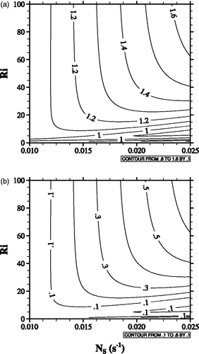
Fig. 8. Differences in (a, b) orographically, (c, d) convectively, and (e, f) both orographically and convectively forced perturbation vertical velocity fields between the cases of N2U10 and N1U10 for the left column and between the cases of N2U20 and N1U20 for the right column. The centre of the convective forcing is located at x = 0 km in (c, d) and x = –10 km in (e, f). The contour line information (unit: m s⁻¹) is given at the bottom of each panel.

From an analysis similar to that about the horizontally symmetric structures of the orographically and convectively forced flows, it is revealed that the relations of the horizontally anti-symmetric structure of the orographically and convectively forced flows are mainly proportional to R₁cosθ₁ – R₂cosθ₂ and R₁cosθ₁ + R₂cosθ₂, respectively. This can also be seen in Fig. 8c and d. For this reason, the mountain waves tend to maintain the horizontally symmetric structure (Fig. 2a and c), and the convectively forced compensating downward motion is strengthened and the maximal vertical velocity moves downstream in the case with stability jump (Fig. 2d and f). The wave reflection at the tropopause has little effect on the positively combined strong updraft in the deep layer upstream of the mountain (from x ∼ –20 km to ∼ –10 km in Fig. 8e and f).

3.3. Gravity-wave momentum fluxes

In a stably stratified atmosphere, orographically/convectively forced internal gravity waves transport momentum vertically. The vertical flux of horizontal momentum can be obtained analytically by using the solutions of u and w, which is defined as (17) $$M\equiv {\rho }_0{\int }_{-\infty }^{\infty }\mathit{\text{uwdx}}.$$(17)

Here, ρ₀ is the reference air density. In this study, we consider the flows forced by the two forcings, and the resultant flows are obtained by the linear superposition of the flows forced by individual forcings. The total momentum flux can thus be divided into three components, (18a) $${\rho }_0{\int }_{-\infty }^{\infty }(u_{\mathrm{m}}+u_{\mathrm{c}})(w_{\mathrm{m}}+w_{\mathrm{c}})dx=M_{\mathrm{m}}+M_{\mathrm{c}}+M_{\text{mc}},$$(18a) where (18b) $$M_{\mathrm{m}}={\rho }_0{\int }_{-\infty }^{\infty }{u}_{\mathrm{m}}{w}_{\mathrm{m}}dx,$$(18b) (18c) $$M_{\mathrm{c}}={\rho }_0{\int }_{-\infty }^{\infty }{u}_{\mathrm{c}}{w}_{\mathrm{c}}dx,$$(18c) (18d) $$M_{\text{mc}}={\rho }_0{\int }_{-\infty }^{\infty }(u_{\mathrm{m}}{w}_{\mathrm{c}}+u_{\mathrm{c}}{w}_{\mathrm{m}})dx.$$(18d)

The total momentum flux has orographically forced component M_m, convectively forced component M_c, and component due to the non-linear interaction between orographically and convectively forced components M_mc. The momentum flux components M_m, M_c, and M_mc in the stratosphere (z > H) are (19) $$M_{\mathrm{m}}=-\frac{{\rho }_0{U}_0^3}{4N_{\mathrm{T}}}{\left(\frac{h_{\mathrm{m}}{N}_{\mathrm{T}}}{U_0}\right)}^2\left(\frac{N_{\mathrm{S}}}{N_{\mathrm{T}}}\right)\left\{R_1^2+R_2^2-2R_1{R}_2\hspace{0.17em}\text{cos}\hspace{0.17em}\left({\theta }_1-{\theta }_2+2{\theta }_{H0}\right)\right\},$$(19) (20) $$\begin{array}{c}{M}_{\mathrm{c}}=-\frac{{\rho }_0{U}_0^3}{N_{\mathrm{T}}}{\left(\frac{g{q}_0{a}_{\mathrm{c}}}{c_p{T}_0{N}_{\mathrm{T}}{U}_0^2}\right)}^2\hspace{0.17em}\text{ln}\hspace{0.17em}\left\{\frac{{\left(a_{\mathrm{c}}+b_{\mathrm{c}}\right)}^2}{4a_{\mathrm{c}}{b}_{\mathrm{c}}}\right\}\\ \underset{\_}{\frac{N_{\mathrm{T}}^2{Z}_{H0}^{-1}}{s^2{\mu }^2}{\left\{Z_{H1}^{\frac{1}{2}}\hspace{0.17em}\text{cos}\hspace{0.17em}\left({\theta }_{10}-{\hspace{0.17em}\text{tan}\hspace{0.17em}}^{-1}\frac{1}{2\mu }\right)-Z_{H2}^{\frac{1}{2}}\hspace{0.17em}\text{cos}\hspace{0.17em}\left({\theta }_{20}-{\hspace{0.17em}\text{tan}\hspace{0.17em}}^{-1}\frac{1}{2\mu }\right)\right\}}^2}\\ \left(\frac{N_{\mathrm{S}}}{N_{\mathrm{T}}}\right)\left\{R_1^2+R_2^2-2R_1{R}_2\hspace{0.17em}\text{cos}\hspace{0.17em}\left({\theta }_1-{\theta }_2+2{\theta }_{H0}\right)\right\},\end{array}$$(20) (21) $$\begin{array}{c}{M}_{\text{mc}}=-\frac{{\rho }_0{U}_0^3}{N_{\mathrm{T}}}\left(\frac{g{q}_0{a}_{\mathrm{c}}}{c_p{T}_0{N}_{\mathrm{T}}{U}_0^2}\right)\left(\frac{h_{\mathrm{m}}{N}_{\mathrm{T}}}{U_0}\right)\\ \underset{}{2a_{\mathrm{m}}\left(c_{\mathrm{c}}-c_{\mathrm{m}}\right)\left\{\frac{1}{{\left(a_{\mathrm{c}}+a_{\mathrm{m}}\right)}^2+{\left(c_{\mathrm{c}}-c_{\mathrm{m}}\right)}^2}-\frac{1}{{\left(b_{\mathrm{c}}+a_{\mathrm{m}}\right)}^2+{\left(c_{\mathrm{c}}-c_{\mathrm{m}}\right)}^2}\right\}}\\ \frac{N_{\mathrm{T}}{Z}_{H0}^{-\frac{1}{2}}}{s\mu }\left\{Z_{H1}^{\frac{1}{2}}\hspace{0.17em}\text{cos}\hspace{0.17em}\left({\theta }_{10}-{\hspace{0.17em}\text{tan}\hspace{0.17em}}^{-1}\frac{1}{2\mu }\right)-Z_{H2}^{\frac{1}{2}}\hspace{0.17em}\text{cos}\hspace{0.17em}\left({\theta }_{20}-{\hspace{0.17em}\text{tan}\hspace{0.17em}}^{-1}\frac{1}{2\mu }\right)\right\}\\ \left(\frac{N_{\mathrm{S}}}{N_{\mathrm{T}}}\right)\left\{R_1^2+R_2^2-2R_1{R}_2\hspace{0.17em}\text{cos}\hspace{0.17em}\left({\theta }_1-{\theta }_2+2{\theta }_{H0}\right)\right\}.\end{array}$$(21)

The orographically forced momentum flux component can be written as (22) $$M_{\mathrm{m}}=-\frac{{\rho }_0{U}_0^3}{4N_{\mathrm{T}}}{\text{Fr}}^{-2}{c}_3.$$(22)

Recall that Fr = U₀/(N_Th_m) is the Froude number. The parameter c₃ = (N_S/N_T){R₁² + R₂² – 2R₁R₂cos(θ₁ – θ₂ + 2θ_H0)} is related to the wave transmission through the tropopause. When N_T = N_S and s = 0, M_m is equal to the momentum flux given in Smith and Lin (1982) in which uniform basic-state wind speed and static stability are considered.

The convectively forced momentum flux component can be written as (23) $$M_{\mathrm{c}}=-\frac{{\rho }_0{U}_0^3}{N_{\mathrm{T}}}{\mu }_{\text{NL}}^2{c}_1{c}_2^2{c}_3.$$(23)

Recall that μ_NL = (gq₀a_c)/(c_pT₀N_TU₀²) is the non-linearity factor of thermally forced internal gravity waves. The parameter c₁ = ln{(a_c + b_c)²/4a_cb_c} is related to the horizontal structure of the convective forcing. The parameter c₂² is related to the basic-state wind speed, tropospheric static stability, and the bottom and top heights of the convective forcing. The transmission related parameter c₃ is also multiplied. When N_T = N_S and s = 0, M_c is equal to the momentum flux given in Chun and Baik (1998) in which uniform basic-state wind speed and static stability are considered.

The component caused by the non-linear interaction between orographically and convectively forced internal gravity waves can be written as (24) $$M_{\text{mc}}=-\frac{{\rho }_0{U}_0^3}{N_{\mathrm{T}}}{\mu }_{\text{NL}}{\text{Fr}}^{-1}\times \frac{2\left(b_{\mathrm{c}}-a_{\mathrm{c}}\right)\left(a_{\mathrm{c}}+b_c+2a_{\mathrm{m}}\right)\left(c_{\mathrm{c}}-c_{\mathrm{m}}\right)}{\left\{{\left(a_{\mathrm{c}}+a_{\mathrm{m}}\right)}^2+{\left(c_{\mathrm{c}}-c_{\mathrm{m}}\right)}^2\right\}\left\{{\left(b_{\mathrm{c}}+a_{\mathrm{m}}\right)}^2+{\left(c_{\mathrm{c}}-c_{\mathrm{m}}\right)}^2\right\}}{c}_2{c}_3.$$(24)

Equation (24)(24) $$M_{\text{mc}}=-\frac{{\rho }_0{U}_0^3}{N_{\mathrm{T}}}{\mu }_{\text{NL}}{\text{Fr}}^{-1}\times \frac{2\left(b_{\mathrm{c}}-a_{\mathrm{c}}\right)\left(a_{\mathrm{c}}+b_c+2a_{\mathrm{m}}\right)\left(c_{\mathrm{c}}-c_{\mathrm{m}}\right)}{\left\{{\left(a_{\mathrm{c}}+a_{\mathrm{m}}\right)}^2+{\left(c_{\mathrm{c}}-c_{\mathrm{m}}\right)}^2\right\}\left\{{\left(b_{\mathrm{c}}+a_{\mathrm{m}}\right)}^2+{\left(c_{\mathrm{c}}-c_{\mathrm{m}}\right)}^2\right\}}{c}_2{c}_3.$$(24) is the geometric average of Eqs. (22)(22) $$M_{\mathrm{m}}=-\frac{{\rho }_0{U}_0^3}{4N_{\mathrm{T}}}{\text{Fr}}^{-2}{c}_3.$$(22) and (23)(23) $$M_{\mathrm{c}}=-\frac{{\rho }_0{U}_0^3}{N_{\mathrm{T}}}{\mu }_{\text{NL}}^2{c}_1{c}_2^2{c}_3.$$(23) except for the parameter related to the horizontal structure, which depends on the location of the convection relative to the mountain and on the horizontal scales of the mountain and convection. The term in the second line of Eq. (21)(21) $$\begin{array}{c}{M}_{\text{mc}}=-\frac{{\rho }_0{U}_0^3}{N_{\mathrm{T}}}\left(\frac{g{q}_0{a}_{\mathrm{c}}}{c_p{T}_0{N}_{\mathrm{T}}{U}_0^2}\right)\left(\frac{h_{\mathrm{m}}{N}_{\mathrm{T}}}{U_0}\right)\\ \underset{}{2a_{\mathrm{m}}\left(c_{\mathrm{c}}-c_{\mathrm{m}}\right)\left\{\frac{1}{{\left(a_{\mathrm{c}}+a_{\mathrm{m}}\right)}^2+{\left(c_{\mathrm{c}}-c_{\mathrm{m}}\right)}^2}-\frac{1}{{\left(b_{\mathrm{c}}+a_{\mathrm{m}}\right)}^2+{\left(c_{\mathrm{c}}-c_{\mathrm{m}}\right)}^2}\right\}}\\ \frac{N_{\mathrm{T}}{Z}_{H0}^{-\frac{1}{2}}}{s\mu }\left\{Z_{H1}^{\frac{1}{2}}\hspace{0.17em}\text{cos}\hspace{0.17em}\left({\theta }_{10}-{\hspace{0.17em}\text{tan}\hspace{0.17em}}^{-1}\frac{1}{2\mu }\right)-Z_{H2}^{\frac{1}{2}}\hspace{0.17em}\text{cos}\hspace{0.17em}\left({\theta }_{20}-{\hspace{0.17em}\text{tan}\hspace{0.17em}}^{-1}\frac{1}{2\mu }\right)\right\}\\ \left(\frac{N_{\mathrm{S}}}{N_{\mathrm{T}}}\right)\left\{R_1^2+R_2^2-2R_1{R}_2\hspace{0.17em}\text{cos}\hspace{0.17em}\left({\theta }_1-{\theta }_2+2{\theta }_{H0}\right)\right\}.\end{array}$$(21) related to the horizontal structures of the mountain and convection is exactly the same as the “cross terms proportional to hQ” in Eq. (65) of Smith and Lin (1982). The sign of the non-linear interaction component depends on the location of the convection relative to the mountain. When the convection centre is equal to the mountain centre (c_c = c_m), M_mc becomes zero. The non-linear interaction component in the case with the convection centre being located upslope (downslope) of the mountain has a positive (negative) value. As a function of the location of the convection relative to the mountain (c_c – c_m), M_mc has an anti-symmetric structure for given parameter values. In the case of c_c – c_m < 0 (c_c – c_m > 0), the positive maximum (negative minimum) of M_mc occurs when 6(c_c – c_m)² = a_c²{(r⁴ + 14r² +1)^1/2 – (r² + 1)}, where r = b_c/a_c. In this study (r = 5), (c_c – c_m)_max/min = ±0.93a_c = ±9.3 km.

Depending on the location of the convection relative to the mountain, the total momentum flux can be increased or decreased due to the orographic–convective interaction. Fig. 9 shows the momentum fluxes forced by the mountain, convection, and orographic–convective interaction as a function of the stratospheric buoyancy frequency and the Richardson number. In this calculation, ρ₀ = 0.7 kg m⁻³ and c_c – c_m = –10 km are used. In an inviscid atmosphere without a critical level, the momentum flux above a forcing does not vary with height and internal gravity waves that transport energy upward have a negative momentum flux (Eliassen and Palm, 1960; Chun and Baik, 1998). At/Near the boundary where the phase angle reversal occurs, the discontinuity of the momentum flux exists. For a given N_S, the magnitude of M_m (M_c) decreases (increases) as Ri increases (Figs. 9a and b). M_c is more sensitive to Ri (also to s) compared to M_m. For a given Ri, both components M_m and M_c increase in magnitude as the stratospheric buoyancy frequency increases. The dependency of the magnitude of M_mc on N_S and Ri is similar to that of M_c (Fig. 9c). As discussed in Section 3.2, the wave reflection at the tropopause strengthens the symmetric (anti-symmetric) structure of the orographically (convectively) forced flows. For this reason, the dependency of each momentum flux component on N_S and Ri is similar to that of R₁cosθ₁ + R₂cosθ₂ on N_S and Ri (Fig. 7). Note that the non-linear interaction component has the same order of magnitude as each of the orographically and convectively forced components.

Fig. 9. Momentum fluxes forced by the (a) mountain, (b) convection, and (c) orographic–convective interaction as a function of the stratospheric buoyancy frequency and the Richardson number. Here, c_c – c_m = –10 km is used.

4. Summary and conclusions

In this study, we theoretically examined orographic–convective flows, gravity-wave reflection, and gravity-wave momentum fluxes in a two-layer atmosphere representing the troposphere and stratosphere. The resultant flows are the linear superposition of orographically forced flows and convectively forced flows. The stability jump between the troposphere and the stratosphere plays an important role in orographic–convective flows. It was found that the gravity-wave reflection at the tropopause strengthens the symmetric structure of the orographically forced internal gravity waves and the anti-symmetric structure of the convectively forced internal gravity waves in the troposphere. The vertical fluxes of horizontal momentum in the stratosphere were analytically obtained. The total momentum flux contains a component related to the non-linear interaction between convectively and orographically forced waves. It was found that the non-linear interaction component has an order of magnitude comparable to each of the orographically and convectively forced components, which can increase or decrease the total momentum flux depending on the location of the convection relative to the mountain. The parameterizations of orographic and convective gravity wave drags have considered both wave components separately. In some situations, however, the interaction component between orographic and convective forcings is not negligible compared to either the orographically forced component or the convectively forced component. The parameterization of the interaction generated gravity wave drag deserves an in-depth investigation.

In this study, we considered orographic–convective flows in a hydrostatic system. In a non-hydrostatic system, orographically and convectively forced internal gravity waves propagate horizontally or slantwise as well as vertically. Some dynamics associated with non-hydrostatic effects on orographically forced flows have been theoretically examined (Wurtele et al., 1987; Keller, 1994). Woo et al. (2013) described non-hydrostatic effects on convectively forced flows using a non-linear dynamical model. Further studies are needed to examine non-hydrostatic effects on orographically and convectively forced flows.

Acknowledgements

The authors are grateful to two anonymous reviewers for providing valuable comments on this study.

Disclosure statement

No potential conflict of interest was reported by the authors.

Additional information

Funding

This work was funded by the Korea Meteorological Administration Research and Development Program under grant [KMIPA 2015–5100 and KMIPA 2015–5190].

References

- Beres, J. H. 2004. Gravity wave generation by a three-dimensional thermal forcing. J. Atmos. Sci. 61, 1805–1815.
- Bretherton, C. 1988. Group velocity and the linear response of stratified fluids to internal heat or mass sources. J. Atmos. Sci. 45, 81–93.
- Bretherton, F. P. 1969. Momentum transport by gravity waves. Q. J. Royal Met. Soc. 95, 213–243.
- Chun, H.-Y. 1995. Enhanced response of a stably stratified two-layer atmosphere to low-level heating. J. Met. Soc. Jpn. 73, 685–696.
- Chun, H.-Y. and Baik, J.-J. 1994. Weakly nonlinear response of a stably stratified atmosphere to diabatic forcing in a uniform flow. J. Atmos. Sci. 51, 3109–3121.
- Chun, H.-Y. and Baik, J.-J. 1998. Momentum flux by thermally induced internal gravity waves and its approximation for large-scale models. J. Atmos. Sci. 55, 3299–3310.
- Chun, H.-Y. and Baik, J.-J. 2002. An updated parameterization of convectively forced gravity wave drag for use in large-scale models. J. Atmos. Sci. 59, 1006–1017.
- Crook, N. A. and Tucker, D. F. 2005. Flow over heated terrain. Part I: linear theory and idealized numerical simulations. Mon. Weather Rev. 133, 2552–2564.
- Davies, H. C. and Schár, C. 1986. Diabatic modification of airflow over a mesoscale orographic ridge: a model study of the coupled response. Q. J. Royal Met. Soc. 112, 711–730.
- Durran, D. R. 1992. Two-layer solutions to Long’s equation for vertically propagating mountain waves: How good is linear theory?. Q. J. Royal Met. Soc. 118, 415–433.
- Eliassen, A. and Palm, E. 1960. On the transfer of energy in stationary mountain waves. Geofys. Publ. 22, 1–23.
- Fueglistaler, S., Haynes, P. H. and Forster, P. M. 2011. The annual cycle in lower stratospheric temperatures revisited. Atmos. Chem. Phys. 11, 3701–3711.
- Han, J.-Y. and Baik, J.-J. 2009. Theoretical studies of convectively forced mesoscale flows in three dimensions. Part I: uniform basic-state flow. J. Atmos. Sci. 66, 947–965.
- Han, J.-Y. and Baik, J.-J. 2010. Theoretical studies of convectively forced mesoscale flows in three dimensions. Part II: shear flow with a critical level. J. Atmos. Sci. 67, 694–712.
- Holton, J. R. 1982. The role of gravity wave induced drag and diffusion in the momentum budget of the mesosphere. J. Atmos. Sci. 39, 791–799.
- Holton, J. R. and Hakim, G. J. 2012. An Introduction to Dynamic Meteorology. 5th ed. Academic Press, Oxford, 552pp.
- Houze, R. A. Jr. 2014. Cloud Dynamics. 2nd ed. Academic Press, Oxford, 432pp.
- Iwasaki, T., Yamada, S. and Tada, K. 1989. A parameterization scheme of orographic gravity wave drag with two different vertical partitionings. Part I: impacts on medium-range forecasts. J. Met. Soc. Jpn. 67, 11–27.
- Jiang, Q. 2003. Moist dynamics and orographic precipitation. Tellus 55A, 301–316.
- Keller, T. L. 1994. Implications of the hydrostatic assumption on atmospheric gravity waves. J. Atmos. Sci. 51, 1915–1929.
- Kim, Y.‐J., Eckermann, S. D. and Chun, H.‐Y. 2003. An overview of the past, present and future of gravity-wave drag parameterization for numerical climate and weather prediction models. Atmos. Ocean 41, 65–98.
- Kirshbaum, D. J. 2013. On thermally forced circulations over heated terrain. J. Atmos. Sci. 70, 1690–1709.
- Lin, Y.-L. 1986. A study of the transient dynamics of orographic rain. Pap. Meteor. Res 9, 20–44.
- Lin, Y.-L. 1987. Two-dimensional response of a stably stratified shear flow to diabatic heating. J. Atmos. Sci. 44, 1375–1393.
- Lin, Y.-L. 2007. Mesoscale Dynamics. Cambridge University Press, Cambridge, 630pp.
- Lin, Y.-L. and Chun, H.-Y. 1991. Effects of diabatic cooling in a shear flow with a critical level. J. Atmos. Sci. 48, 2476–2491.
- Lin, Y.-L. and Li, S. 1988. Three-dimensional response of a shear flow to elevated heating. J. Atmos. Sci. 45, 2987–3002.
- Lin, Y.-L. and Smith, R. B. 1986. Transient dynamics of airflow near a local heat source. J. Atmos. Sci. 43, 40–49.
- Lindzen, R. S. 1981. Turbulence and stress due to gravity wave and tidal breakdown. J. Geophys. Res. 86, 9707–9714.
- McFarlane, N. A. 1987. The effect of orographically excited gravity wave drag on the general circulation of the lower stratosphere and troposphere. J. Atmos. Sci. 44, 1775–1800.
- Palmer, T. N., Shutts, G. J. and Swinbank, R. 1986. Alleviation of a systematic westerly bias in general circulation and numerical weather prediction models through an orographic gravity wave drag parameterization. Q. J. Royal Met. Soc. 112, 1001–1039.
- Pierrehumbert, R., T. 1986. An essay on the parameterization of orographic gravity wave drag. In: Proceedings of Seminar/Workshop on Observation, Theory, and Modeling of Orographic Effects. United Kingdom, ECMWF, 251–378.
- Queney, P. 1948. The problem of airflow over mountain: a summary of theoretical studies. Bull. Am. Meteor. Soc. 29, 16–26.
- Raymond, D. J. 1972. Calculation of airflow over an arbitrary ridge including diabatic heating and cooling. J. Atmos. Sci. 29, 837–843.
- Reisner, J. M. and Smolarkiewicz, P. K. 1994. Thermally forced low Froude number flow past three-dimensional obstacles. J. Atmos. Sci. 51, 117–133.
- Smith, R. B. 1980. Linear theory of stratified hydrostatic flow past an isolated mountain. Tellus 32, 348–364.
- Smith, R. B. and Lin, Y.-L. 1982. The addition of heat to a stratified airstream with application to the dynamics of orographic rain. Q. J. Royal Met. Soc. 108, 353–378.
- Song, I.-S. and Chun, H.-Y. 2005. Momentum flux spectrum of convectively forced internal gravity waves and its application to gravity wave drag parameterization. Part I: theory. J. Atmos. Sci. 62, 107–124.
- Song, I.-S. and Chun, H.-Y. 2008. A Lagrangian spectral parameterization of gravity wave drag induced by cumulus convection. J. Atmos. Sci. 65, 1204–1224.
- Song, I.-S., Chun, H.-Y., Garcia, R. R. and Boville, B. A. 2007. Momentum flux spectrum of convectively forced internal gravity waves and its application to gravity wave drag parameterization. Part II: impacts in a GCM (WACCM). J. Atmos. Sci. 64, 2286–2308.
- Tian, W. and Parker, D. J. 2003. A modeling study and scaling analysis of orographic effects on boundary layer shallow convection. J. Atmos. Sci. 60, 1981–1991.
- Woo, S., Baik, J.-J., Lee, H., Han, J.-Y. and Seo, J. M. 2013. Nonhydrostatic effects on convectively forced mesoscale flows. J. Korean Met. Soc. 23, 293–305.
- Wurtele, M. G., Sharman, R. D. and Keller, T. L. 1987. Analysis and simulations of a troposphere-stratosphere gravity wave model. Part I. J. Atmos. Sci. 44, 3269–3281.