Uncertainty and sensitivity of wave-induced sea surface roughness parameterisations for a coupled numerical weather prediction model

Abstract

The impact of wave-induced sea surface roughness (SSR) parameterisation methods on tropical cyclone (TC) forecasts in a coupled numerical weather prediction (NWP) model is investigated by comparing the results of sensitivity experiments. A wind-dependent SSR parameterisation as a control experiment and five wave-induced SSRs parameterised by wave age, wave steepness, wave-induced stress, and input wave age, which are the most commonly used to estimate the air–sea exchange coefficients, are used in our comparative sensitivity experiments. In this study, we clearly show the magnitude of uncertainties given by the different choice of roughness parameterisations. Our results show that the choice of SSR parameterisation has a considerable influence on the atmospheric boundary layer and wave conditions, leading to a significant difference in both the forecast of TC intensity and the wave fields. The air-sea momentum and enthalpy transports are modified by the differences in exchange coefficients between the various SSR parameterisation methods, which result in differences in frictional convergence, and variation in the amount of energy input to the TC, thus changing the TC intensity. This process is linked to the alteration of the wind fields and then the wave fields. Comparison of observation data with the results obtained via several SSR parameterisation methods indicates that wind speed, and consequently energy transfer to the waves, is reduced by increased SSR, resulting in smaller wave heights. In addition, the increased SSR produces enhanced turbulent heat flux and rainfall rates by inducing an increase in thermal and moisture exchange coefficients.

Keywords:

• wave-induced sea surface roughness parameterisations
• coupled numerical weather prediction
• tropical cyclone
• air–sea interaction

1. Introduction

It is well known that air–sea interaction has a considerable influence on many meteorological phenomena, and in particular, plays a vital role in the occurrence of extreme weather events originating from the ocean, such as a heavy snowfall event in the coastal regions and tropical cyclones (TCs). In recent years, a number of workshops and projects have focused on the impact of an interactive ocean on improved weather forecasting. Some of these, such as the Joint Global Ocean Data Assimilation Experiment (GODAE) OceanView-Working Group for Numerical Experimentation (WGNE) workshop (2013), and the Joint Weather and Climate Research Programme (JWCRP), have made significant progress regarding the operational atmosphere–wave–seaice–ocean coupled prediction systems for the short to medium range. Moreover, in the European Centre for Medium-Range Weather Forecasts (ECMWF) Workshop on Ocean-Waves, Cavaleri et al. (2012) emphasised that ‘The coupling of waves to the atmosphere is an obvious and necessary step toward a unified approach to improve the description of the atmospheric boundary layer and the forecast of ocean waves’. This approach had already been shown by Janssen et al. (2004) to improve both atmosphere and surface wave forecasts on a global scale.

The effect of sea state on surface momentum flux in numerical weather prediction (NWP) models has been recognised for some time now (Janssen, 1989). Sea surface roughness (SSR) is one of the important factors for understanding the relation between surface wind and momentum flux from air to sea (Drennan et al., 2005). The SSR, which is induced by ocean waves, plays a role in the air–sea transfer of momentum, heat, moisture, gasses, sea-spray aerosols, etc. Many studies have been carried out using atmosphere–ocean–wave coupled models (Doyle, 1995, 2002; Lionello et al., 1998; Desjardins et al., 2000; Lalbeharry et al., 2000; Cavaleri et al, 2012; Olabarrieta et al., 2012; Renault et al., 2012). The common purpose of these studies was to evaluate the results obtained by using a more realistic representation of the exchange of momentum and enthalpy between the sea surface and the overlying atmosphere. According to these studies, coupled models give slightly better results than uncoupled models, but many noticeable differences are exhibited during extreme storms. Because TCs, such as typhoons and hurricanes, are one among most destructive of all severe meteorological phenomena, they need to be predicted accurately. Furthermore, the TC-induced ocean waves can affect the TC structure and intensity, especially the variability of surface winds (e.g. Chen et al., 2013; Kwon and Kim, 2017).

In order to better understand the spatial distribution of integrated mean wave properties and the directional spectra, Chen and Curcic (2016) used a coupled atmosphere–wave–ocean model for TCs and showed that the predictions of ocean waves in TCs were verified very well against both in situ and satellite observations. Moreover, the coupled modelling studies by Chen et al. (2013) and Chen and Curcic (2016) have shown that TC-induced ocean waves are highly complex and asymmetric in terms of wave heights and propagation directions around a moving storm (Curcic et al., 2016). Therefore, the exchange coefficients for momentum and enthalpy could also be directionally affected by the wave orientation. These studies demonstrate that the coupled systems of atmosphere–ocean–wave models have been built to improve TC forecasts, capture air–sea interactions, and better represent ocean responses and TCs impacts. Consequently, the impact of ocean waves on TC intensity forecasting was gradually recognised by operational meteorologists and the coupled atmosphere–wave model has therefore been in use at many operational centres (e.g. Järvenoja and Tuomi, 2002; Sattler et al., 2002; Janssen et al., 2005, Chen et al., 2007; Warner et al., 2010).

The most important objective of an operational NWP model is to accurately predict extreme weather events, and thus to give forewarning and enable preparation for the potential damage they can cause (Kim and Jin, 2016). Among extreme weather events, it is particularly difficult to accurately predict the intensity and structure of a TC by comparing the track forecast. TC tracks are ultimately affected by large-scale flows. The errors in TC track prediction have steadily decreased over the past several decades due to the use of increasing horizontal and vertical model resolution, improvements in model physics and advanced data assimilation (Rogers et al., 2003; Gentry and Lackmann, 2010). However, the variation in intensity and structure in a TC mainly depends on processes occurring on much smaller scales. These include smaller scale convection and multi-scale interactions (Molinari and Dudek, 1992), along with other environmental factors such as vertical wind shear (Emanuel et al., 2004; Rhome et al., 2006), and sea surface temperature (SST) (Weidinger et al., 2000). In addition to these environmental factors, the exchange process of momentum and enthalpy between atmosphere and ocean is also known to be one of the key factors controlling the intensity and structure of a TC (Montgomery et al., 2010; Green and Zhang, 2013; Kwon and Kim, 2017). Ooyama (1969) found that the TC intensity is positively (negatively) proportional to the enthalpy (momentum) exchange coefficient through sensitivity experiments using a numerical model. In addition, Emanuel (1986) and many follow up works derived that the quasi-steady state TC intensity is dependent on the ratio between the momentum exchange coefficient ($C_D$) and heat exchange coefficient ($C_H$), which is consistent with Ooyama (1969).

Considering that $C_D$ and $C_H$ are functions of the SSR, air–sea exchange processes may be differently affected by various sea-state dependent SSR parameterisation methods. Plenty of formulae for estimation of SSR have so far been suggested and discussed, because (1) it is not possible to directly observe the fluxes over the ocean in high wind speeds, (2) the variability of the exchange coefficients is quite large over the ocean (e.g. Toffoli et al., 2012), and (3) there could be differences in measurement methods and significant errors in observations (e.g. Montgomery et al., 2010; Kwon and Kim, 2017). The impact of coupling may depend on the various SSR parameterisation methods, even though the exchanged parameters are well-defined based on the physics of air–sea interactions. A number of studies on the effect of surface waves on the air–sea transfer process have been carried out, especially at high wind speeds, such as during typhoons and hurricanes (e.g. Olabarrieta et al., 2012; Renault et al., 2012). Although air–sea coupling is useful for improving TC intensity forecasts, the wave-dependent SSR parameterisation at the air–sea interface can have a strong influence on the simulated TC structure and intensity, which is the focus of this study. In order to investigate the impacts of several wave-induced SSR parameterisation methods on weather forecasting and to quantify the uncertainties given by the different roughness parameterisations, we carried out a series of comparative experiments for a single TC case.

In this context, the impact of various wave-induced SSR parameterisation methods on the forecasting of the TC intensity and wave fields is investigated in a case study of Typhoon Sanba (201216) (hereafter, Sanba) using a coupled atmosphere–wave model. In this study, we are trying to identify the magnitude of uncertainties given by the different choice of SSR parameterisations. The performance of the different SSR parameterisation methods may provide valuable guidance as to how the prediction of TC activity in a coupled NWP modelling system varies with parameterisation method. The paper is organised as follows. The model used in this study and the experiment design are described in Section 2. The results including the estimated SSR, the effect of the SSR on the TC, and wave and enthalpy flux are given in Section 3. Finally, Section 4 presents a summary and the conclusion.

2. Methodology

2.1. Model description

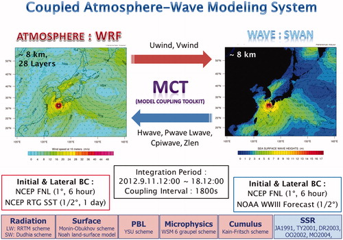
To investigate the impact of various wave-induced SSR parameterisation methods on a coupled NWP model, we used the Coupled Ocean-Atmosphere-Wave-Sediment Transport (COAWST) modelling system (Warner et al., 2010). In this study, the modelling system consisted of two model components: atmosphere (Weather Research and Forecasting, WRF) and ocean wave (Simulating Waves Nearshore, SWAN). WRF was coupled to SWAN through the Model Coupling Toolkit (Jacob et al., 2005; Larson et al., 2005; Warner et al., 2008).

The WRF model is a fully compressible and non-hydrostatic model that uses Arakawa-C grid staggering for the horizontal coordinate and terrain-following hydrostatic pressure for the vertical (Skamarock et al., 2008). A short listing of the parameterisations and schemes used in the present study is as follows: the Yonsei University planetary boundary layer (YSU-PBL) scheme, the Kain-Fritsch cumulus parameterisation scheme, the WRF single-moment 6-class (WSM6) microphysics scheme, the Dudhia scheme for shortwave radiation, the Rapid Radiative Transfer Model (RRTM) scheme for longwave radiation, and the Noah land-surface model. The surface fluxes of momentum and enthalpy are calculated using the Monin-Obukhov similarity method. In this study, several wave-induced SSR parameterisation schemes are used for estimation of the bulk exchange coefficients for calculating the surface fluxes. More detailed descriptions of the bulk exchange coefficients and the SSR parameterisations are given in the following sections and in Appendix A, respectively. The model had an 8 km horizontal resolution, and 28 vertical layers extending to 50 hPa. The initial and boundary conditions of the meteorological fields were prepared using 6-hourly National Centers for Environmental Prediction (NCEP) Final (FNL) Operational Global Analysis data (NCEP/NWS/NOAA/U.S. Department of Commerce, 2000), with a 1° resolution and a daily Real-Time Global (RTG) SST analysis (Gemmill et al., 2007), provided by NCEP with a 0.5° resolution.

The SWAN model is a third-generation spectral wave model specifically designed for shallow water simulation (Booij et al., 1999). The model is based on the wave action balance equation, and includes a number of physical processes, such as refraction, shoaling, diffraction, wind–wave generation, redistribution of the energy spectrum due to nonlinear wave–wave interactions, and dissipation due to wave breaking, whitecapping, and bottom friction. For the present study, bottom dissipation was parameterised using the Madsen et al. (1988) formulation. The Janssen formulation (Janssen, 1989, 1991) for wind wave growth/whitecapping was used with a coefficient of 4.5 to determine the rate of whitecapping dissipation. SWAN was run in the same grid as WRF. The spectral directional resolution was 10°. The lowest and highest discrete frequencies used in the calculation were 0.0285 Hz and 1.1726 Hz, respectively, and the grid resolution in the frequency space between the lowest and the highest discrete frequencies was 41. The initial spectra were computed by running the model in stationary mode using the FNL winds. Boundary conditions were updated using the 3-hourly global WAVEWATCH III model (Tolman, 1991), which is operationally run at the National Oceanic and Atmospheric Administration (NOAA). The surface wind used in the Janssen closure model (Janssen, 1989) for the exponential energy transfer from the atmosphere to the wave field was provided by WRF.

A schematic diagram of the coupled atmosphere–wave modelling system, brief descriptions of the parameterisation schemes, and model set-up considered in this study are shown in Fig. 1. The two-way coupling between the models involves the transfer of surface wind from WRF to SWAN, and the transfer of wave fields from SWAN to WRF every 30 minutes. The latter includes wave height (Hwave), wave period (Pwave), wavelength (Lwave), SSR estimated in the wave model using the total stress (Zlen), and input wave age (Cpiwave), depending on selected SSR parameterisation methods in each sensitivity experiment (Fig. 1). In both component models of the coupled system, the model domain covers the Northwestern Pacific Ocean region from 15°N to 55°N, 105°E to 165°E. Model simulation was carried out for Sanba using an 8-day forecast from 12 UTC on September 11, 2012.

Fig. 1. A schematic diagram of the coupled atmosphere–wave modelling system, and brief descriptions of the parameterisation schemes and model set-up considered in this study. The exchange variables between the models are surface wind (Uwind and Vwind) from WRF to SWAN, and the wave fields, such as wave height (Hwave), wave period (Pwave), wavelength (Lwave), SSR estimated in the wave model using the total stress (Zlen), and input wave age (Cpiwave), depending on the selected SSR parameterisation method, from SWAN to WRF.

2.2. Air–sea exchange coefficients

The bulk surface fluxes of momentum ($\tau )$, sensible heat ($SH$), and latent heat ($LH$) are given by: (1) $$\tau =-\rho C_D{\left(U\right)}^2$$(1) (2) $$SH=\rho c_p{C}_{H}U\mathrm{\Delta }\theta$$(2) (3) $$LH=\rho L_v{C}_{Q}U\mathrm{\Delta }q$$(3) where $\rho$ is the density of air; U is wind speed at a reference height of 10 m, $z;\mathrm{}{c}_p$ is the specific heat capacity at constant pressure; $\mathrm{\Delta }\theta$ and $\mathrm{\Delta }q$ are the differences in potential temperature and the specific humidity between the surface and a reference height, respectively; $L_v$ is the enthalpy of vaporisation per unit mass; and $C_D$, $C_H$_, and $C_Q$ are bulk transfer coefficients for momentum, sensible heat, and moisture, respectively. The bulk transfer coefficients can be expressed using the Monin-Obukhov similarity theory, as follows: (4) $$C_D=\frac{k}{ln\left(\frac{z}{z_0}\right)-{\psi }_m\left(\frac{z}{L}\right)}\times \frac{k}{ln\left(\frac{z}{z_0}\right)-{\psi }_m\left(\frac{z}{L}\right)}$$(4) (5) $$C_H=\frac{k}{ln\left(\frac{z}{z_0}\right)-{\psi }_m\left(\frac{z}{L}\right)}\times \frac{k}{ln\left(\frac{z}{z_T}\right)-{\psi }_h\left(\frac{z}{L}\right)}$$(5) (6) $$C_Q=\frac{k}{ln\left(\frac{z}{z_0}\right)-{\psi }_m\left(\frac{z}{L}\right)}\times \frac{k}{ln\left(\frac{z}{z_Q}\right)-{\psi }_h\left(\frac{z}{L}\right)}$$(6) where $k$ is the von Kármán constant; $z_0$, $z_T$, and $z_Q$ are the roughness lengths of momentum, sensible heat, and latent heat, respectively; ${\psi }_m$ and ${\psi }_h$ are the universal functions for momentum and enthalpy, which are functions of the atmospheric stability and become zero under neutral conditions; and $L$ is the Obukhov length scale.

In this study, air–sea transfer coefficients were estimated through the surface layer module of WRF, using the revised MM5 surface layer scheme (Jiménez et al., 2012). In the MM5 similarity scheme, stability functions from Dyer and Hicks (1970), Paulson (1970) and Webb (1970) are used and the correction terms are computed by considering the stability classes following Zhang and Anthes (1982). The momentum roughness length ($z_0$) was calculated using various SSR parameterisation methods. The thermal roughness length ($z_T$) was set equal to $z_0$ and the moisture roughness length ($z_Q$) was calculated as: (7) $$z_Q={\left({z_0}^{-1}+\kappa u_{\mathrm{*}}{K_a}^{-1}\right)}^{-1}$$(7) where $k$ is the von Kármán constant, $u_{\mathrm{*}}$ is the frictional velocity, and $K_a$ is the background molecular diffusivity set to $2.4\times {10}^{-5}{\mathrm{m}}^2{\mathrm{s}}^{-1}$ (Carlson and Boland, 1978).

It should be noted that heat and moisture transports are also modified due to the various SSR parameterisation methods, because both $C_H$ and $C_Q$ depend on $z_0$.

2.3. Experiment design

Because of problems, such as difficulty in observation, observation errors, and differences in measurement methods, locations and time, many different formulae for estimation of SSR, depending on the wind speed (e.g. Large and Pond, 1981; Fairall et al., 2003; Powell et al., 2003; Donelan, 2004; Jarosz et al., 2007; Large and Yeager, 2009; Hersbach, 2011; Edson et al., 2013) or on the sea state (e.g. Janssen, 1989, 1991; Taylor and Yelland, 2001; Oost et al., 2002; Drennan et al., 2003; Moon et al., 2004), have been proposed and discussed. When the sea state is not considered in estimation of SSR, the formulation proposed by Charnock (1955), in which SSR is proportional to wind speed, is widely used. Among the formulae which do consider sea state, the most widely adopted are those based on wave age dependency ($z_{ch}=\frac{{gz}_0}{{u_{\mathrm{*}}}^2}=f\left(\frac{C_p}{u_{\mathrm{*}}}\right)$, Stewart, 1974). In this study, typically-used SSR parameterisation methods were selected to identify the uncertainties given by the various wave-induced SSR parameterisations, and the sensitivity of the TC forecasts to them was examined. A wind-dependent SSR parameterisation as the control experiment (AW-CTL) and five wave-induced SSRs parameterised by wave age (AW-DR2003), wave steepness (AW-TY2001), both wave age and wave steepness (AW-OO2002), wave-induced stress (AW-JA1991), and input wave age (AW-MO2004), were used in the sensitivity experiments. These experiments were intended to investigate how the selected SSR parameterisation method influences the forecast of the TC track and intensity [sea level pressure (SLP)], strength (wind speed), wave heights, surface roughness, sea surface stresses, and precipitation. To investigate the effect of the different SSR parameterisation schemes, all the formulae were implemented in the surface module of WRF. A more detailed explanation of these parameterisation methods is provided in Appendix A.

2.4. Typhoon Sanba (201216)

The coastal area around the Northwestern Pacific Ocean has often been damaged by storm surges, heavy precipitation, and strong winds due to repeated strong typhoons. Sanba, the typhoon used for the present study, was the strongest typhoon worldwide in 2012. Its minimum central pressure reached 900 hPa, and its maximum 1-minute sustained wind speed was 77 m/s. The typhoon generated wind waves more than 15 m in significant wave height and severely damaged coastal structures. It originated as a low pressure atmospheric system in the Pacific Ocean on September 9, 2012. As it moved north, it grew bigger and intensified into a category 5 super-typhoon, with the highest 10-minute average wind speed of 57 m/s and a minimum pressure of 900 hPa on September 13–14 (black line in Fig. 2b,c). It made landfall on the Korean Peninsula on September 17 and travelled across it. Coastal areas around the Northwestern Pacific Ocean, such as Korea, China, and Japan, were influenced by the typhoon, which was accompanied by strong winds of over 20 m/s, heavy precipitation of 60 mm/h, and a maximum surge level up to 2 m.

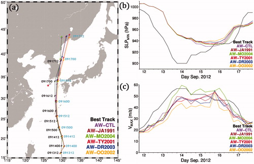
Fig. 2. (a) Best track and time evolutions of (b) minimum sea level pressure and (c) maximum wind speed of Typhoon Sanba, provided from JTWC (black line) and simulated from each experiment (coloured lines). The red star in (a) indicates the position of Buoy 22107 for the time-series of wind and wave height in Fig. 8.

3. Results

3.1. Estimated SSR

As previously mentioned, ocean waves can have a significant impact on the exchange of momentum and enthalpy fluxes at the air–sea interface. The effect of ocean waves on these fluxes can be explained using an SSR that is dependent on the sea state as well as on the wind speed. Figure 4 shows the spatial distribution of the SSR estimated by each experiment in the coupled modelling system on 00 UTC September 16, when the typhoon passed over the southern East China Sea. The horizontal distribution of the SSR obtained through the Charnock relation (i.e. AW-CTL) follows the typical wind speed pattern around the typhoon, as the roughness is taken to be a function of wind speed only. In all simulations, the SSR shows a similar spatial distribution but differences of several times of magnitude in the regions associated with high wave activity. AW-OO2002 produced the highest ocean surface roughness, while AW-MO2004 produced the lowest. The SSRs estimated in AW-TY2001 and AW-DR2003, which are dependent on the wind wave spectrum, show typical wind speed patterns with wave-like structures, because part of the momentum from the wind stress is propagated away by the ocean waves. Furthermore, because AW-OO2002 considers the effect of both wave age and steepness, it represents an SSR field that blends the variations estimated in AW-DR2003 and AW-TY2001. The SSR affects not only the dynamics of the atmospheric boundary layer by surface variations on the momentum flux and therefore the wave growth, but it also impacts on the thermodynamics by increasing or decreasing the heat and moisture fluxes from the ocean to the atmosphere. As a result, the difference in SSR estimated by the various SSR parameterisations can lead to changes in the conditions of the atmospheric boundary layer and ocean wave fields.

3.2. Effect of the SSR on the TC intensity and wave fields

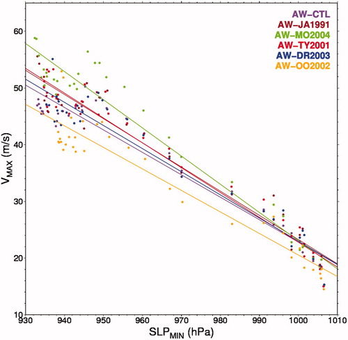
The response of Sanba to different SSR parameterisations is presented in Fig. 2. This shows a comparison of the observed track, strength, and intensity of Sanba with the results predicted by each experiment, which depicts the positions with minimum SLP, and time evolution of minimum SLP and maximum wind speed. The tracks do not differ significantly between the experiments. In all simulations, the predicted track is close to the observed track, and is not sensitive to the wave-induced SSR parameterisation methods, agreeing with previous studies such as Doyle (2002) and Zambon et al. (2014a,b). The track of a TC is mainly governed by large-scale flows, not meso-scale processes influenced by ocean coupling (Marks and Shay, 1998). However, as the forecast lead time increases, all the tracks predicted by each experiment deviate slightly from the observations, and Sanba moved northward faster than the observations as it approached the shallow water area (Figs. 2a and 8). The minimum SLP calculated in most of the experiments was overestimated, while the maximum winds were underestimated, except in AW-MO2004. The deviation was larger in AW-OO2002 than in the others. An interesting thing is that there is a difference between the strength and intensity forecasts; the minimum SLP varies by about 10 hPa but the maximum wind varies more than 10 m/s. In addition, there is the large and early change in the maximum wind, compared with minimum SLP (Fig. 2b,c). This may indicate that the SSR parameterisation has more impact on the surface winds. Figure 3 shows the pressure–wind relationship (PWR) estimated from each experiment. The PWR lines of the experiment results shows different behaviours in terms of slope. Namely, the slope of the pressure–wind lines changes with a different SSR parameterisation. The slope change in the pressure-wind–lines indicates that the maximum wind speeds are different for the same central pressure value. Because the maximum wind speed of a typhoon is proportional to the radial pressure gradient, not to the minimum SLP value itself, the maximum wind can be different at the same central pressure value. Therefore, the radial pressure gradient needs to become bigger to create higher wind speeds at a given central pressure. This may result in that the size of a storm is smaller. From this perspective, the PWR in the experiments suggests a change in the size of the storm (Kwon and Kim, 2017).

Fig. 3. Plots of minimum sea level pressure vs maximum 10 m wind speed predicted from each experiment.

It is worth to note that our simulation of the TC does not have as low of a pressure and makes landfall a little earlier than the observations. One of possible reasons for the differences in minimum SLP and a little earlier landfall between simulations and observations might be initial condition and time used for the experiments (e.g. Kurihara et al., 1995; Wang, 1998; Wu et al., 2000, 2006). In this study, the forecasting period is 7 days (168 hours) in all experiments without any data assimilations and bogus vortex for initial condition, in order to investigate the impact of only SSR parameterisation methods. The forecast skill varies with forecast lead time and, in general, it decreases with the increasing lead time. Moreover, the differences between the simulations and observations are growing as the forecast lead time increases. This may be one disadvantage of this study. But that can be de-emphasised by focusing on the processes that occur due to the changes of the SSR. This can be considered as a test case to see what the order of magnitude changes will occur by varying the SSR.

Figure 5 compares the horizontal distribution of SLP and wind fields simulated by each experiment at 00 UTC September 16. Together with Fig. 4 this demonstrates that the wind field is highly sensitive to SSR. The wind speeds are significantly reduced by an increase in SSR (Fig. 4). In addition to the effect on surface winds, SSR also affects the prediction of ocean wave intensity in a coupled NWP system. The spatial distribution of significant wave height derived from each experiment at 00 UTC September 16 is shown in Fig. 6. The SSR itself should be related to the wave height; an increase in wave height makes the SSR high. However, severe reduction in significant wave height was predicted in AO-OO2002 which produced the highest ocean surface roughness. Figure 7 displays the $C_D/C_H$ ratio estimated from each experiment at 00 UTC September 16. The horizontal distributions of the $C_D/C_H$ ratio correspond well with those of the SSR (Fig. 4); the largest (smallest) value in AW-OO2002 (AW-MO2004). According to the wind-induced surface heat exchange (WISHE) mechanism (Emanuel, 1986; Rotunno and Emanuel, 1987), when the $C_D/C_H$ ratio becomes large, the TC intensity becomes weak (Figs. 5 and 7). Thus, it reduces the intensity of the system leading to the smaller wave height (Figs. 6 and 7). The reduction in significant wave height is induced by less energy transferring to the wave as a result of an increase in SSR. The spatial distribution of significant wave height corresponds to that of the wind speed, due to the decrease in wind speed over regions with large SSR. As a result, the severe reduction in wind associated with the large SSR in AW-OO2002 acts to decrease the significant wave height. The reduction in surface wind speed and consequently wave height is consistent with previous atmosphere–wave numerical experiments (Weber et al., 1993; Doyle, 1995, 2002; Janssen and Viterbo, 1996; Lionello et al., 1998; Desjardins et al., 2000; Zhang and Perrie, 2001; Warner et al., 2010).

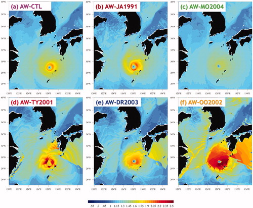
Fig. 4. Spatial distribution of sea surface roughness estimated by each experiment at 00 UTC September 16, 2012; (a) AW-CTL, (b) AW-JA1991, (c) AW-MO2004, (d) AW-TY2001, (e) AW-DR2003, and (f) AW-OO2002.

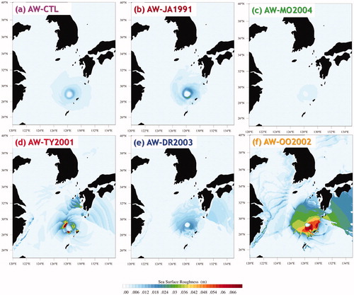
Fig. 5. Horizontal distribution of 10 m wind fields (arrows and colour shading) and sea level pressure (contours) calculated from each experiment at 00 UTC September 16, 2012; (a) AW-CTL, (b) AW-JA1991, (c) AW-MO2004, (d) AW-TY2001, (e) AW-DR2003, and (f) AW-OO2002.

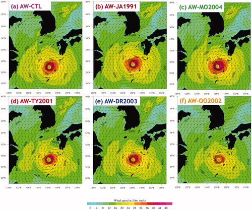
Fig. 6. The same as Fig. 5, but for wind fields (arrows and contours) and significant wave height (colour shading).

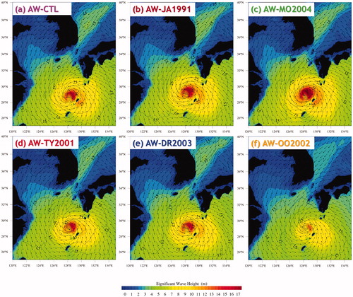
Fig. 7. The same as Fig. 5, but for the $C_D/C_H$ ratio.

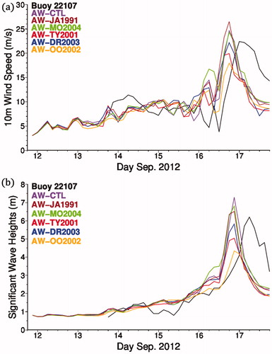
The wind speeds and significant wave heights predicted by each experiment were compared with the observations. Figure 8 represents the time series of the measured and computed wind speeds and significant wave heights at Buoy 22107 (33.0833°N, 126.033°E, as indicated by the red star in Fig. 2a). On September 17, Sanba impacted the station, resulting in a 23 m/s wind speed and a 6 m peak significant wave height. In all experiments, the simulated typhoon passes through the station about 12 hours earlier than the observed time, because it moves faster than observed as it approaches the coastal region (Fig. 2). The choice of SSR parameterisation results in approximately 10 m/s difference in the maximum wind speed and 3 m difference in the maximum significant wave height. The maximum wind speed depends on the ratio of $C_D$ to $C_H$ according to the WISHE mechanism. When the enhanced SSR parameterisation is included (e.g. AW-OO2002), the maximum wind and wave intensities are significantly reduced in the coupled model. For example, AW-OO2002 yielded the highest reduction in wind intensity and wave heights. AW-MO2004 produced the results closest to the observed values, as shown by comparing the track and intensity (Fig. 2).

Fig. 8. Time series of measured (black lines) and simulated (coloured lines) (a) wind speed and (b) significant wave height at Buoy 22107 (33.0833°N, 126.033°E), shown as a red star in Fig. 2a.

3.3. Effect of the SSR on the enthalpy flux

TC intensity and evolution are influenced by two main atmosphere–ocean interaction processes mentioned above; exchange of momentum and enthalpy fluxes due to SSR (Ooyama, 1969; Emanuel, 1986, 1995; Rotunno and Emanuel, 1987; Zhang and Perrie, 2001; Bao et al., 2012; Bryan, 2012; Kwon and Kim, 2017). The enhanced SSR due to wind waves results in momentum transfer from the atmosphere to the ocean, and then surface wind speed decreases via this interaction. On the other hand, an increase in enthalpy flux from the ocean to the atmosphere produces an intensification of the synoptic system by serving as energy input (Kwon and Kim, 2017).

The effect of surface gravity waves on air–sea heat flux is important as well, especially the effect of sea spray in TC conditions (Liu et al., 2010, 2012). Although it is hard to figure out the effect of surface gravity waves on air–sea transfer by considering SSR only, heat and moisture transports are also modified by the SSR parameterisation methods because the exchange coefficients for heat and moisture are a function of momentum roughness length as well as thermal and moisture roughness as seen in Eqs. (5)(5) $$C_H=\frac{k}{ln\left(\frac{z}{z_0}\right)-{\psi }_m\left(\frac{z}{L}\right)}\times \frac{k}{ln\left(\frac{z}{z_T}\right)-{\psi }_h\left(\frac{z}{L}\right)}$$(5) and (6)(6) $$C_Q=\frac{k}{ln\left(\frac{z}{z_0}\right)-{\psi }_m\left(\frac{z}{L}\right)}\times \frac{k}{ln\left(\frac{z}{z_Q}\right)-{\psi }_h\left(\frac{z}{L}\right)}$$(6) . According to Kang and Kwon (2016), precipitation bands and low-pressure systems are mainly influenced by changes in the heat exchange coefficient. However, changes in momentum flux also have an influence on heat and moisture transport via wind speed changes that are dependent on SSR, although this is an indirect impact. In addition, Lionello et al. (1998) found that heat and moisture fluxes increase when they are computed using the same wave-dependent roughness as applied for momentum flux, and decrease when they are computed using the Charnock (1955) relation, where they are a function of wind speed only, and the effects become proportionally larger for extreme storms.

As previously mentioned, the SSR modulates the intensity of the moisture and heat fluxes and the consequent convection, resulting in a change in precipitation rate. Because of enthalpy flux change due to the SSR parameterisation methods, the lower atmosphere can become warmer and moister, which contributes to destabilisation of the air mass, resulting in changes to the precipitation pattern. The spatial distribution of the daily mean latent and sensible heat fluxes on September 16, and the 12-hour accumulated precipitation on September 15 and 16, computed in each experiment are shown in Figs. 9 and 10, respectively. The increased SSR enhanced the turbulent heat flux (sum of sensible and latent heat flux) from the ocean to the atmosphere, which is to be expected from Eqs. (2)(2) $$SH=\rho c_p{C}_{H}U\mathrm{\Delta }\theta$$(2) , (3)(3) $$LH=\rho L_v{C}_{Q}U\mathrm{\Delta }q$$(3) , (5)(5) $$C_H=\frac{k}{ln\left(\frac{z}{z_0}\right)-{\psi }_m\left(\frac{z}{L}\right)}\times \frac{k}{ln\left(\frac{z}{z_T}\right)-{\psi }_h\left(\frac{z}{L}\right)}$$(5) , and (6)(6) $$C_Q=\frac{k}{ln\left(\frac{z}{z_0}\right)-{\psi }_m\left(\frac{z}{L}\right)}\times \frac{k}{ln\left(\frac{z}{z_Q}\right)-{\psi }_h\left(\frac{z}{L}\right)}$$(6) . As a result, the amount of precipitation increased due to the large heat and moisture fluxes. The turbulent heat flux and the 12-hour accumulated precipitation have similar spatial distributions in all experiments, while their intensity and area depend on the SSR parameterisation methods. The amounts of turbulent heat flux and 12-hour accumulated precipitation produced by AW-OO2002, in which the largest momentum roughness length was predicted, are larger than in the other simulations as expected (Fig. 4). The thermal and moisture roughness lengths produced by AW-MO2004 have smaller values than in the other simulations because the momentum roughness length estimated is relatively small (Fig. 4). However, the amounts of turbulent heat flux and precipitation in AW-MO2004 are comparable to the other simulations. This can be partly explained by the change of wind field due to the momentum roughness length. The enthalpy flux is also a function of wind speed, as well as thermal and moisture roughness length, as expressed in Eqs. (2)(2) $$SH=\rho c_p{C}_{H}U\mathrm{\Delta }\theta$$(2) and (3)(3) $$LH=\rho L_v{C}_{Q}U\mathrm{\Delta }q$$(3) . The amount and spatial distribution of precipitation predicted by AW-MO2004 are rather close to the observed value; that is, the amount of 12-hour accumulated precipitation along the coast of Korea is underestimated in the sensitivity experiments, except for AW-MO2004 and AW-OO2002. In AW-MO2004 and AW-OO2002, the intensity and location of precipitation are improved; a large amount of 12-hour accumulated precipitation is obtained along the southwestern coast of Korea in AW-OO2002 and the band along the south coast of Korea simulated in AW-MO2004 is in good agreement with the observations (Fig. 10). The increase in turbulent heat flux due to the SSR increase contributes to the intensification of warm and moist air through the increase in sensible and latent heat flux from the ocean to atmosphere, which is a primary energy source for TCs. According to the WISHE mechanism, the TC intensity depends on the $C_D/C_H$ ratio. The WISHE mechanism tells that if the $C_D/C_H$ ratio becomes large, the TC intensity becomes weak. 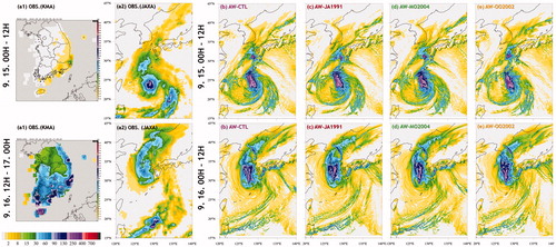Therefore, the increase in enthalpy exchange coefficient through the SSR increase can strengthen the TC intensity when the $C_D$ increase has little impact in reducing it (e.g. Kwon and Kim, 2017). In the present application, when the effect of wave-induced SSR is included, precipitation close to the observed values is obtained, especially in the coastal region of Korea; for example, the band along the east coast and the frontal angle across the peninsula (Fig. 10). When the effect of the waves was included, Sanba absorbed more moisture and turbulent heat fluxes due to the increase in SSR.

Fig. 9. Horizontal distribution of daily mean latent (top row) and sensible (bottom row) heat fluxes calculated from experiments on September 16; (a) AW-CTL, (b) AW-JA1991, (c) AW-MO2004, (d) AW-OO2002.

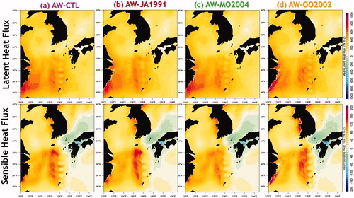
Fig. 10. Comparison between measured and modelled 12 hours accumulated precipitation (shaded in colour): (a1) surface observations provided from the Korea Meteorological Administration (KMA), (a2) global rainfall observed by satellites, which is provided from the Japan Aerospace eXploration Agency (JAXA) Global Satellite Mapping of Precipitation (GSMap), (b) AW-CTL, (c) AW-JA1991, (d) AW-MO2004, (e) AW-OO2002.

4. Summary and conclusion

Recent studies on the impact of an interactive ocean on NWP model predictions have shown that coupled air–sea interaction is an important physical mechanism in determining the intensity and structure of extreme weather events, and that the inclusion of an interactive ocean in an NWP model can improve weather prediction, particularly for localised severe weather (Kim and Jin, 2016). Consequently, it is regarded as natural to include a wave model in the NWP model to accurately predict extreme weather events, such as extreme TCs.

The wave effect is a well-known physical process in air-sea interaction. It is usually represented by parameterising SSR. However, the wave-induced SSR parameterisation under the high wind regime is still widely uncertain because the observation is sporadic. Understanding the physical processes is still qualitative. Our results show that the parameterisation methods for wave-dependent SSR at the air-sea interface have a strong influence on simulated TC structure and intensity, even though air-sea coupling in a TC is useful for improving model intensity forecasts. This is because SSR parameterisation has an influence on air–sea momentum and enthalpy exchange processes, which are regarded as the primary energy sink and source of a TC (Kwon and Kim, 2017).

From this perspective, we attempt to show the magnitude of uncertainties given by the different choice of roughness parameterisations. In order to estimate SSR, many experimental formulae, depending on wind speed or sea surface state, have been proposed and discussed. In the present study, we selected the most commonly-used schemes to examine the impact of various wave-induced SSR parameterisation methods on extreme weather prediction, and examined the sensitivity of TC forecasts using a coupled regional atmosphere–wave modelling system. Five wave-induced SSRs parameterised by wave age, wave steepness, both wave age and wave steepness, wave-induced stress, and input wave age were used in the sensitivity experiments, along with a wind-dependent SSR parameterisation as a control experiment.

In all the simulations, the SSRs estimated from each experiment show similar spatial distributions, but differences of several orders of magnitude in regions associated with high wave activity. The typhoon’s predicted track in all simulations is close to the observed one and is not sensitive to the SSR parameterisation schemes, which is consistent with previous studies. As the forecast lead time increases, all the tracks predicted by the experiments deviated slightly from the observed track, and the typhoon moved northward faster than in the observations as it approached the shallow water area. However, our results show that the various parameterisation schemes used to estimate SSR lead to significant differences in both typhoon intensity and wave fields in the coupled atmosphere–wave model. This indicates that air–sea interaction is modified by the SSR parameterisation method. In other words, the SSR parameterisation scheme affects the aerodynamic turbulent roughness length, air–sea momentum and enthalpy fluxes, resulting in changes in the wind velocity profiles. Consequently, SSR influences the ocean surface wind stress, which also affects the intensity of the ocean waves.

A change in drag coefficients due to the SSR parameterisation methods caused a change in typhoon intensity because of frictional convergence changes (Kwon and Kim, 2017), which resulted in alteration of wind fields, and then wave fields. Regarding the effect on surface winds, significant wave height reduction is also induced by SSR increase, which affects the intensity of ocean waves by decreasing the wind speed over large SSR regions. Comparison of model wave heights with observed data from a buoy indicates that the increase in SSR reduced the wind speed, and consequently energy transfer to the waves, resulting in smaller wave heights. In addition, the increase in SSR produced an increase in turbulent heat flux and rainfall rates, and the change of momentum flux also has an influence on heat and moisture transport via wind speed changes due to SSR, although this is an indirect impact.

This work is based on a single TC forecast and therefore, the validation requires a large number of TC forecasts and the current study does not guarantee that the use of wave age based parameterisation improves the skill of TC intensity or structure prediction. However, the results clearly show the magnitude of uncertainties given by the different choice of SSR parameterisations, which is the main objective of this study. It should be noted that significant difference in both the forecast of TC intensity and the wave fields is caused by the choice of SSR parameterisation even though air–sea coupling is useful for improving TC intensity forecasts. In this study, our results underlined the uncertainty and sensitivity of wave-induced SSR parameterisations for a coupled NWP model.

Although the results in this study are deduced from the case of a single typhoon, the SSR parameterisation method which considered the input wave age clearly showed improvement. This improvement is demonstrated in the TC intensity, associated wave fields, and precipitation in the coupled NWP model. These results suggest that this parameterisation is more suitable for the present application than the others. However, this cannot be generalised too much, but this finding may be applicable empirically to the forecast of TC in some sense. In the future, we plan to conduct further analysis using other case studies. In addition, sea spray has a significant impact on air–sea heat and moisture fluxes, and the evaporation caused by it favours for TC intensification by enhancing the surface enthalpy flux. Therefore, the impact of SSR parameterisation incorporating a sea spray factor will also be examined using a coupled NWP model. We expect that further study will enable us to gain a better understanding of air–sea interactions and lead to improvements in weather prediction, particularly for localised severe weather. And finally, it may provide valuable guidance as to which methods are useful for predicting weather phenomena in a coupled NWP modelling system.

Acknowledgements

This work has been carried out through the project ‘Research and Development for Korea Meteorological Administration (KMA) Weather, Climate, and Earth system Services’ funded by the National Institute of Meteorological Sciences (NIMS) (NIMS-2016-3100). J.-H. Moon was supported by the National Research Foundation of Korea (NRF) grant funded by the Korea government (MSIP) (NRF-2016R1A2B4008219). Typhoon Sanba track and intensity data are from the Joint Typhoon Warning Center (JTWC), USA. The precipitation over the Korean Peninsula and buoy observation data related to and used in this study are available for free download from https://data.kma.go.kr/cmmn/main.do. The global rainfall maps observed by satellites are provided from the Japan Aerospace eXploration Agency (JAXA) Global Satellite Mapping of Precipitation (GSMap) from http://sharaku.eorc.jaxa.jp/GSMap/. The authors express their gratitude to Prof. Il-Ju Moon for his valuable comments and suggestions on this work.

Appendix A

Sea surface roughness parameterisations

When wave fields are not used for calculation of sea surface fluxes in the WRF (AW-CTL), the SSR is computed using the formulation proposed by Charnock (1955). However, when sea states are considered in the WRF, there are five available expressions for including wave-induced roughness at the sea surface. In the COAWST modelling system, three closure models have been implemented for wave-induced SSR. The first is the wave steepness-based model of Taylor and Yelland (2001), which provides a good estimation of SSR under swell conditions, but it produces underestimates in young windseas (Drennan et al., 2005). The second closure model is that of Drennan et al. (2003), which is based on wave age, and neglects wave steepness, and shows a better performance for young sea states. The third is the model of Oost et al. (2002), in which the effect of the wave steepness is indirectly considered along with the wave age.

In addition to these, two more parameterisations were implemented in this study; those of Janssen (1989, 1991) and Moon et al. (2004). When the parameterisation of Janssen (1989, 1991) is used, the SSR is estimated in the wave model using the total stress, which is expressed as the sum of turbulent, wave-induced, and viscous stress, and then transferred to the atmosphere model. Moon et al. (2004) used a fully coupled wave-wind model and proposed a different relationship dependent on the input wave age, which is the wave age determined by the peak frequency of the wind energy input. In this study, the regression constants for the parameterisation of Moon et al. (2004) are used as suggested by Fan et al. (2012).

The simulation names, expressions, references, and regression coefficients of the six parameterisations used for the SSRs considered in this study are briefly described as follows:

References

- Bao, J.-W., Gopalakrishnan, S. G., Michelson, S. A., Marks, F. D. and Montgomery, M. T. 2012. Impact of physics representations in the HWRFX model on simulated hurricane structure and wind–pressure relationships. Mon. Weather Rev. 140, 3278–3299. doi: 10.1175/MWR-D-11-00332.1.
- Booij, N., Ris, R. C. and Holthuijsen, L. H. 1999. A third-generation wave model for coastal regions, part I. Model description and validation. J. Geophys. Res. 104, 7649–7666. doi: 10.1029/98JC02622.
- Bryan, G. H. 2012. Effects of surface exchange coefficients and turbulence length scales on the intensity and structure of numerically simulated hurricanes. Mon. Weather Rev. 140, 1125–1143. doi: 10.1175/MWR-D-11-00231.1.
- Carlson, T. N. and Boland, F. E. 1978. Analysis of urban-rural canopy using a surface heat flux/temperature model. J. Appl. Meteor. 17, 998–1013. doi: 10.1175/1520-0450(1978)017<0998:AOURCU>2.0.CO;2.
- Cavaleri, L., Fox-Kemper, B. and Hemer, M. 2012. Wind waves in the coupled climate system. Bull. Amer. Meteor. Soc. 93, 1651–1661. doi: 10.1175/BAMS-D-11-00170.1.
- Cavaleri, L., Roland, A., Dutour, M., Bertotti, L. and Torrisi, L. 2012. On the coupling of COSMO to WAM, In Proceedings of the ECMWF Workshop on Ocean-Waves.
- Chen, S. S. and Curcic, M. 2016. Ocean surface waves in Hurricane Ike (2008) and Superstorm Sandy (2012): Coupled modelling and observations. Ocean Model 103, 161–176. doi: 10.1016/j.ocemod.2015.08.005.
- Chen, S. S., Price, J. F., Zhao, W., Donelan, M. A. and Walsh, E. J. 2007. The CBLAST-Hurricane program and the next-generation fully coupled atmosphere-wave-ocean models for hurricane research and prediction. Bull. Am. Meteor. Soc. 88, 311–317. doi: 10.1175/BAMS-88-3-311.
- Chen, S. S., Zhao, W., Donelan, M. A. and Tolman, H. L. 2013. Directional wind-wave coupling in fully coupled atmosphere-wave-ocean models: Results from CBLAST-Hurricane. J. Atmos. Sci. 70, 3198–3215. doi: 10.1175/JAS-D-12-0157.1.
- Charnock, H. 1955. Wind stress on a water surface. Q. J. Royal Met. Soc. 81, 639–640. doi: 10.1002/qj.49708135027.
- Curcic, M., Chen, S. S., and Özgökmen, T.M. 2016. Hurricane-induced ocean waves and stokes drift and their impacts on surface transport and dispersion in the Gulf of Mexico. Geophys. Res. Lett. 43, 2773–2781. doi: 10.1002/2015GL067619.
- Desjardins, S., Mailhot, J. and Lalbeharry, R. 2000. Examination of the impact of a coupled atmospheric and ocean wave system. Part I: Atmospheric aspects. J. Phys. Oceanogr. 30, 402–401. doi: 10.1175/1520-0485(2000)030<0402:EOTIOA>2.0.CO;2.
- Donelan, M. A., Haus, B. K., Reul, N., Plant, W. J., Stiassnie, M., Graber, H. C., Brown, O. B. and Saltzman, E. S. 2004. On the limiting aerodynamic roughness of the ocean in very strong winds. Geophys. Res. Lett. 31, L18306. doi: 10.1029/2004GL019460.
- Doyle, J. D. 1995. Coupled ocean wave/atmosphere mesoscale model simulations of cyclogenesis. Tellus 47, 766–788. doi: 10.1034/j.1600-0870.1995.00119.x.
- Doyle, J. D. 2002. Coupled atmosphere–ocean wave simulations under high wind conditions. Mon. Weather Rev. 130, 3087–3099. doi:1 doi: 10.1175/1520-0493(2002)130<3087:CAOWSU>2.0.CO;2.
- Drennan, W. M., Graber, H. C., Hauser, D. and Quentin, C. 2003. On the wave age dependence of wind stress over pure wind seas. J. Geophys. Res. 108, 8062. doi: 10.1029/2000JC000715.
- Drennan, W. M., Taylor, P. K. and Yelland, M. J. 2005. Parameterizing the sea surface roughness. J. Phys. Oceanogr. 35, 835–848. doi: 10.1175/JPO2704.1.
- Dyer, A. J. and Hicks, B. B. 1970. Flux-gradient relationships in the constant flux layer. Q. J. R. Met. Soc. 96, 715–721. doi: 10.1002/qj.49709641012.
- Edson, J. B., Jampana, V., Weller, R. A., Bigorre, S. P., Plueddemann, A. J., and co-authors. 2013. On the exchange of momentum over the open ocean. J. Phys. Oceanogr. 43, 1589–1610. doi: 10.1175/JPO-D-12-0173.1.
- Emanuel, K. A. 1986. An air-sea interaction theory for tropical cyclones. Part I: Steady-state maintenance. J. Atmos. Sci. 43, 585–605. doi: 10.1175/1520-0469(1986)043<0585:AASITF>2.0.CO;2.
- Emanuel, K. A. 1995. Sensitivity of tropical cyclones to surface exchange coefficients and a revised steady-state model incorporating eye dynamics. J. Atmos. Sci. 52, 3969–3976. doi: 10.1175/1520-0469(1995)052<3969:SOTCTS>2.0.CO;2.
- Emanuel, K., DesAutels, C., Holloway, C. and Korty, R. 2004. Environmental control of tropical cyclone intensity. J. Atmos. Sci. 61, 843–858. doi: 10.1175/1520-0469(2004)061<0843:ECOTCI>2.0.CO;2.
- Fan, Y., Lin, S.-J., Held, I. M., Yu, Z. and Tolman, H. L. 2012. Global ocean surface wave simulation using a coupled atmosphere-wave model. J. Clim. 25, 6233–6252. doi: 10.1175/JCLI-D-11-00621.1.
- Fairall, C. W., Bradley, E. F., Hare, J. E., Grachev, A. A. and Edson, J. B. 2003. Bulk parameterization of air-sea fluxes: Updates and verification for the COARE algorithm. J. Clim. 16, 571–591. doi: 10.1175/1520-0442(2003)016<0571:BPOASF>2.0.CO;2.
- Gemmill, W., Katz, B. and Li, X. 2007. Daily Real-Time, Global Sea Surface Temperature - High-Resolution Analysis: RTG_SST_HR. NOAA, Camp Springs, MD.
- Gentry, M. S. and Lackmann, G. M. 2010. Sensitivity of simulated tropical cyclone structure and intensity to horizontal resolution. Mon. Weather Rev. 138, 688–704. doi: 10.1175/2009MWR2976.1.
- Green, B. W. and Zhang, F. 2013. Impacts of air–sea flux parameterizations on the intensity and structure of tropical cyclones. Mon. Weather Rev. 141, 2308–2232. doi: 10.1175/MWR-D-12-00274.1.
- Hersbach, H. 2011. Sea surface roughness and drag coefficient as functions of neutral wind speed. J. Phys. Oceanogr. 41, 247–251. doi: 10.1175/2010JPO4567.1.
- Jacob, R., Larson, J. and Ong, E. 2005. M×N Communication and parallel interpolation in community climate system model version 3 using the model coupling toolkit. Int. J. High Perform. Comput. Appl 19, 293–307. doi: 10.1177/1094342005056116.
- Janssen, P. A. E. M. 1989. Wave-induced stress and the drag of air flow over sea waves. J. Phys. Oceanogr. 19, 745–754. doi: 10.1175/1520-0485(1989)019<0745:WISATD>2.0.CO;2.
- Janssen, P. A. E. M. 1991. Quasi-linear theory of win-wave generation applied to wave forecasting. J. Phys. Oceanogr. 21, 1631–1642. doi: 10.1175/1520-0485(1991)021<1631:QLTOWW>2.0.CO;2.
- Janssen, P. A. E. M., Bidlot, J.-R., Abdalla, S. and Hersbach, H. 2005. Progress in ocean wave forecasting at ECMWF. ECMWF Tech. Memo. 478. [Available online https://www.ecmwf.int/sites/default/files/elibrary/2005/10187-progress-ocean-wave-forecasting-ecmwf.pdf]
- Janssen, P. A. E. M., Saetra, O., Wettre, C. and Hersbach, H. 2004. Impact of the sea state on the atmosphere and ocean. Ann. Hydrogr. 3, 3.1–3.23.
- Janssen, P. A. E. M. and Viterbo, P. 1996. Ocean waves and the atmospheric climate. J. Clim. 9, 1269–1287. doi: 10.1175/1520-0442(1996)009<1269:OWATAC>2.0.CO;2.
- Jarosz, E., Mitchell, D. A., Wang, D. W. and Teague, W. J. 2007. Bottom-up determination of air-sea momentum exchange under a major tropical cyclone. Science 315, 1707–1709. doi: 10.1126/science.1136466.
- Järvenoja, S. and Tuomi, L. 2002. Coupled atmosphere-wave model for FMI and FIMR. Hirlam Newslett. 40, 9–22.
- Jiménez, P. A., Dudhia, J., González-Rouco, J. F., Navarro, J., Montávez, J. P. and co-authors. 2012. A revised scheme for the WRF surface layer formulation. Mon. Weather Rev. 140, 898–918. doi: 10.1175/MWR-D-11-00056.1.
- Joint GODAE OceanView/WGNE workshop on short- to medium-range coupled prediction for the atmosphere-wave-sea-ice-ocean. Status, needs and challenges, 19–21 March 2013. [Available online http://www.godae-oceanview.org/outreach/meetings-workshops/taskteam-meetings/coupled-prediction-workshop-gov-wgne-2013/ (accessed 22 July 2015)].
- Kang, J.-Y. and Kwon, Y. C. 2016. Impacts of air-sea exchange coefficients on snowfall events over the Korean Peninsula. J. Atmos. Sol.-Terr. Phys. 146, 1–15. doi: 10.1016/j.jastp.2016.04.017.
- Kim, T. and Jin, E. K. 2016. Impact of an interactive ocean on numerical weather prediction: A case of a local heavy snowfall event in eastern Korea. J. Geophys. Res. Atmos. 121, 8243–8253. doi: 10.1002/2016JD024763.
- Kurihara, Y., Bender, M. A., Tuleya, R. E. and Ross, R. J. 1995. Improvements in the GFDL hurricane prediction system. Mon. Weather Rev. 123, 2791–2801. doi: 10.1175/1520-0493(1995)123<2791:IITGHP>2.0.CO;2.
- Kwon, Y. C. and Kim, T. 2017. Impact of air-sea exchange coefficients on the structure and intensity of tropical cyclones. Terr. Atmos. Ocean. Sci. 28, 345–356. doi: 10.3319/TAO.2016.11.16.01.
- Lalbeharry, R., Mailhot, J., Desjardins, S., and and Wilson, L. 2000. Examination of the impact of a coupled atmospheric and ocean wave system. Part II: Ocean wave aspects. J. Phys. Oceanogr. 30, 402–415. doi: 10.1175/1520-0485(2000)030<0402:EOTIOA>2.0.CO;2.
- Large, W. G. and Pond, S. 1981. Open ocean momentum flux measurements in moderate to strong winds. J. Phys. Oceanogr. 11, 324–336. doi: 10.1175/1520-0485(1981)011<0324:OOMFMI>2.2.CO;2.
- Large, W. G. and Yeager, S. G. 2009. The global climatology of an interannually varying air-sea flux data set. Clim. Dyn. 33, 341–364. doi: 10.1007/s00382-008-0441-3.
- Larson, J., Jacob, R. and Ong, E. 2005. The Model Coupling Toolkit: A new Fortran90 toolkit for building multi-physics parallel coupled models. Int. J. High Perform. Comput. Appl. 19, 277–292. doi: 10.1177/1094342005056115.
- Lionello, P., Malguzzi, P. and Buzzi, A. 1998. Coupling between the atmospheric circulation and ocean wave field: an idealized case. J. Phys. Oceanogr. 28, 161–177. doi: 10.1175/1520-0485(1998)028<0262:CBTACA>2.0.CO;2.
- Liu, B., Guan, C., Xie, L. and Zhao, D. 2012. An investigation of the effects of wave state and sea spray on an idealized typhoon using an air-sea coupled modeling system. Adv. Atmos. Sci. 29, 391–406. doi: 10.1007/s00376-011-1059-7.
- Liu, B., Liu, H., Xie, L., Guan, C. and Zhao, D. 2010. A coupled atmosphere–wave–ocean modeling system: simulation of the intensity of an idealized tropical cyclone. Mon. Weather Rev. 139, 132. 100827132423068, doi: 10.1175/2010MWR3396.1.
- Madsen, O. S., Poon, Y. K. and Graber, H. C. 1988. Spectral wave attenuation by bottom friction: Theory, Proc. ASCE 21st Int. Conf. Coastal Engineering (ICCE), Malaga, Spain, ASCE, 492–504, doi: 10.1061/9780872626874.035.
- Marks, F. and Shay, L. K. 1998. Landfalling tropical cyclones: forecast problems and associated research opportunities. Bull. Am. Meteorol. Soc. 79, 305–323. doi: 10.1175/1520-0477(1998)079<0305:LTCFPA>2.0.CO;2.
- Molinari, J. and Dudek, M. 1992. Parameterization of convective precipitation in mesoscale numerical models: a critical review. Mon. Weather Rev. 120, 326–344. doi: 10.1175/1520-0493(1992)120<0326:POCPIM>2.0.CO;2
- Montgomery, M. T., Smith, R. K. and Nguyen, S. V. 2010. Sensitivity of tropical-cyclone models to the surface drag coefficient. Q. J. R. Meteorol. Soc. 136, 1945–1953. doi: 10.1002/qj.702.
- Moon, I.-J., Ginis, I. and Hara, T. 2004. Effect of surface waves on Charnock coefficient under tropical cyclones. Geophys. Res. Lett. 31, L20302. doi: 10.1029/2004GL020988.
- National Centers for Environmental Prediction/National Weather Service/NOAA/U.S. Department of Commerce 2000. NCEP FNL Operational Model Global Tropospheric Analyses, continuing from July 1999. https://doi.org/10.5065/D6M043C6, Research Data Archive at the National Center for Atmospheric Research, Computational and Information Systems Laboratory, Boulder, Colo. (Updated daily) Accessed 7 Feb. 2016.
- Olabarrieta, M., Warner, J. C., Armstrong, B., Zambon, J. B. and He, R. 2012. Ocean-atmosphere dynamics during Hurricane Ida and Nor'Ida: An application of the coupled ocean-atmosphere-wave-sediment transport (COAWST) modeling system. Ocean Modell. 43–44, 112–137. doi: 10.1016/j-ocemod.2011.12.008.
- Oost, W. A., Komen, G. J., Jacobs, C. M. J. and Van Oort, C. 2002. New evidence for a relation between wind stress and wave age from measurements during ASGAMAGE. Bound. Lay. Meteorol. 103, 409–438. doi: 10.1023/A:1014913624535.
- Ooyama, K. 1969. Numerical simulation of the life cycle of tropical cyclones. J. Atmos. Sci. 26, 3–40. doi: 10.1175/1520-0469(1969)026<0003:NSOTLC>2.0.CO;2
- Paulson, C. A. 1970. The Mathematical representation of wind speed and temperature profiles in the unstable atmospheric surface layer. J. Appl. Meteor. 9, 857–861. doi: 10.1175/1520-0450(1970)009<0857:TMROWS>2.0.CO;2
- Powell, M. D., Vickery, P. J. and Reinhold, T. A. 2003. Reduced drag coefficient for high wind speeds in tropical cyclones. Nature 422, 279–283. doi: 10.1038/nature01481.
- Renault, L., Chiggiato, J., Warner, J. C., Gomez, M., Vizoso, G. and Tintoré, J. 2012. Coupled atmosphere-ocean-wave simulations of a storm event over the Gulf of Lion and Balearic Sea. J. Geophys. Res. 117, C09019. doi: 10.1029/2012JC007924.
- Rhome, J. R., Sisko, C. A. and Knabb, R. D. 2006. On the calculation of vertical shear: An operational perspective. Preprints: 27th Conference on Hurricanes and Tropical Meteorology. https://ams.confex.com/ams/27Hurricanes/techprogram/paper_108724.htm
- Rogers, R., Chen, S., Tenerelli, J. and Willoughby, H. 2003. A numerical study of the impact of vertical shear on the distribution of rainfall in Hurricane Bonnie (1998). Mon. Weather Rev. 131, 1577–1599. doi: 10.1175/2546.1.
- Rotunno, R. and Emanuel, K. A. 1987. An air-sea interaction theory for tropical cyclones. Part II: Evolutionary study using a nonhydrostatic axisymmetric numerical model. J. Atmos. Sci. 44, 542–561. doi: 10.1175/1520-0469(1987)044<0542:AAITFT>2.0CO;2.
- Sattler, K., J., She, B. H., Sass, L., Laursen, L., Landberg, M Nielsen. and co-authors. 2002. Enhanced description of the wind climate in Denmark for determination of wind resources, Scientific Report, 02-09, Danish Meteorological Institute.
- Skamarock, W., J. B., Klemp, J., Dudhia, D. O., Gill, D. M., Barker, M. G Duda. and co-authors. 2008. A description of the advanced research WRF version 3, NCAR Tech. Note, NCAR/TN-4751STR. Natl. Cent. For Atmos. Res., Boulder, Colo., doi: 10.5065/D68S4MVH.
- Stewart, R. W. 1974. The air-sea momentum exchange. Boundary-Layer Meteorol. 6, 151–167. doi: 10.1007/BF00232481.
- Taylor, P. K. and Yelland, M. J. 2001. The dependence of sea surface roughness on the height and steepness of the waves. J. Phys. Oceanogr. 31, 572–590. doi: 10.1175/1520-0485(2001)031<0572:TDOSSR>2.0.CO;2.
- Toffoli, A., Loffredo, L., Le Roy, P., Lefevre, J.-M. and Babanin, A. V. 2012. On the variability of sea drag in finite water depth. J. Geophys. Res. 117, C00J25, doi: 10.1029/2011JC007857.
- Tolman, H. L. 1991. A third-generation model for wind waves on slowly varying, unsteady, and inhomogeneous depths and currents. J. Phys. Oceanogr. 21, 782–797. doi: 10.1175/1520-0485(1991)021<0782:ATGMFW>2.0.CO;2.
- Wallace, J. M., Mitchell, T. P. and Deser, C. 1989. The influence of sea surface temperature on surface wind in the eastern equatorial Pacific: Seasonal and interannual variability. J. Clim. 2, 1492–1499. doi: 10.1175/1520-0442(1989)002<1492:TIOSST>2.0.CO;2.
- Wang, Y. 1998. On the bogusing of tropical cyclones in numerical models: The influence of vertical structure. Meteorol. Atmos. Phys. 65, 153–170.
- Warner, J. C., Armstrong, B., He, R. and Zambon, J. B. 2010. Development of a coupled ocean-atmosphere-wave sediment transport (COAWST) modeling system. Ocean Model. 35, 230–244. doi: 10.1016/j.ocemod.2010.07.010.
- Warner, J. C., Perlin, N. and Skyllingstad, E. D. 2008. Using the model coupling toolkit to couple earth system models. Environ. Model. Softw. 23, 1240–1249. doi: 10.1016/j.envsoft.2008.03.002.
- Webb, E. K. 1970. Profile relationships: The log-linear range, and extension to strong stability. Q. J. R. Met. Soc. 96, 67–90. doi: 10.1002/qj.49709640708.
- Weber, S. L., von Storch, H., Viterbo, P. and Zambresky, L. 1993. Coupling an ocean wave model to an atmospheric general circulation model. Clim. Dyn. 9, 63–61. doi: 10.1007/BF00210009.
- Weidinger, T., Pinto, J. and Horvath, L. 2000. Effects of uncertainties in universal functions, roughness length, and displacement height on the calculation of surface layer fluxes. Meteorol. Z. 9, 139–154.
- Wu, C.-C., Bender, M. and Kurihara, Y. 2000. Typhoon forecasts with the GFDL hurricane model: Forecast skill and comparison of predictions using AVN and NOGAPS global analyses. J. Meteorol. Soc. Jpn. 78, 777–788. doi: 10.2151/jmsj1965.78.6_777.
- Wu, C.-C., Chou, K., Wang, Y. and Kuo, Y. 2006. Tropical cyclone initialization and prediction based on four-dimensional variational data assimilation. J. Atmos. Sci. 63, 2383–2395. doi: 10.1175/JAS3743.1.
- Wu, J. 1980. Wind-stress coefficients over sea surface near neutral conditions: A revisit. J. Phys. Oceanogr. 10, 727–740. doi: 10.1175/1520-0485(1980)010<0727:WSCOSS>2.0.CO;2.
- Zambon, J. B., He, R. and Warner, J. C. 2014. Investigation of hurricane Ivan using the coupled ocean–atmosphere–wave–sediment transport (COAWST) model. Ocean Dyn. 64, 1535–1554. doi: 10.1007/s10236-014-0777-7.
- Zambon, J. B., He, R. and Warner, J. C. 2014b. Tropical to extratropical: Marine environmental changes associated with Superstorm Sandy prior to its landfall. Geophys. Res. Lett. 2014, GL061357. doi: 10.1002/2014GL061357. http://onlinelibrary.wiley.com/doi/10.1002/2014GL061357/full.
- Zhang, D. and Anthes, R. A. 1982. A high-resolution model of the planetary boundary layer-sensitivity tests and comparisons with SESAME-79 data. J. Appl. Meteorol. 21, 1594–1609. doi: 10.1175/1520-0450(1982)021<1594:AHRMOT>2.0.CO;2.
- Zhang, Y. and Perrie, W. 2001. Feedback mechanism for the atmosphere and ocean surface. Bound. Lay. Meteorol 100, 321–348. doi: 10.1023/A:1018996505248.