On the instabilities of tropical cyclones generated by cloud resolving models

Abstract

An approximate method is developed for finding and analysing the main instability modes of a tropical cyclone whose basic state is obtained from a cloud resolving numerical simulation. The method is based on a linearised model of the perturbation dynamics that distinctly incorporates the overturning secondary circulation of the vortex, spatially inhomogeneous eddy diffusivities, and diabatic forcing associated with disturbances of moist convection. Although a general formula is provided for the latter, only parameterisations of diabatic forcing proportional to the local vertical velocity perturbation and modulated by local cloudiness of the basic state are implemented herein. The instability analysis is primarily illustrated for a mature tropical cyclone representative of a category 4 hurricane. For eddy diffusivities consistent with the fairly conventional configuration of the simulation that generates the basic state, perturbation growth is dominated by a low azimuthal wavenumber instability having greatest asymmetric kinetic energy density in the lower tropospheric region of the inner core of the vortex. The characteristics of the instability mode are inadequately explained by nondivergent 2D dynamics. Moreover, the growth rate and modal structure are sensitive to reasonable variations of the diabatic forcing. A second instability analysis is conducted for a mature tropical cyclone generated under conditions of much weaker horizontal diffusion. In this case, the linear model predicts a relatively fast high-wavenumber instability that is insensitive to the parameterisation of diabatic forcing. The prediction is in very good quantitative agreement with a previously published analysis of how the instability develops in a cloud resolving model on the way to creating mesovortices slightly inward of the central part of the eyewall.

Keywords:

• tropical cyclones
• instabilities
• numerical modeling

1. Introduction

Satellite and radar images of mature tropical cyclones commonly reveal deformed eyewalls and mesovortices along the periphery of the eye. There has been longstanding interest in understanding how such features develop and whether the process appreciably affects the temporal trend of vortex intensity. One plausible explanation for the emergence of prominent waves and mesovortices involves an instability of the local circular shear flow. Although such an explanation is prevalent in the literature, there has been limited progress in advancing an instability theory for realistically modelled tropical cyclones.

Basic insights have been gained through the study of idealised two-dimensional (2D) models. Such models show that a vorticity annulus similar to that on the inward edge of an eyewall is usually unstable. The onset of perturbation growth may involve the mutual amplification of counter-propagating vortex Rossby waves or a destabilising wave-critical layer interaction. Depending on specifics, the instability may generate robust arrays of mesovortices or engender transient turbulence that thoroughly redistributes inner core vorticity into a centralised monopole (Schubert et al., 1999; Kossin and Schubert, 2001). The latter transformation may appreciably deepen the central pressure deficit while diminishing the maximum azimuthally averaged wind speed (ibid). Adding simplified parameterisations of diabatic forcing (moist convection) to a nondivergent 2D model or a shallow-water system generally modifies the development of an instability and the coinciding change of vortex intensity. Details depend on the parameterisation, and published results on the topic (Rozoff et al., 2009; Hendricks et al., 2014; Lahaye and Zeitlin, 2016) await rigorous comparison to more realistic theories and numerical simulations.

Additional insights have been gained from the study of three-dimensional (3D) stratified vortices whose basic states do not possess secondary circulations. The dominant modes of instability often resemble their 2D counterparts but differ in quantitative details [Nolan and Montgomery, 2002 (NM02)]. The qualitative similarities can extend beyond wave growth to nonlinear mesovortex formation and potential vorticity mixing (Hendricks and Schubert, 2010). On the other hand, adding vertical structure to the vortex introduces the possibility of baroclinic instability (Kwon and Frank, 2005). Moreover, instability mechanisms involving the interactions of vortex Rossby waves and inertia-gravity waves become potentially relevant in the parameter regime of a major hurricane (Schecter and Montgomery, 2003, 2004; Hodyss and Nolan, 2008; Menelaou et al., 2016; Schecter and Menelaou, 2017).

The final step toward a realistic perturbation theory is to generalise a 3D model to incorporate moisture and secondary circulation into the basic state of the vortex. The inclusion of cloud coverage alone has the effect of substantially reducing static stability (Durran and Klemp, 1982). In principle, such reduction can alter the structure and growth rate of the linear eigenmode associated with an instability (Schecter and Montgomery, 2007 (SM07); Menelaou et al., 2016). The importance of the secondary circulation to the prevailing mechanism of perturbation growth is presently unclear. Although secondary circulations are known to significantly influence the inner core instabilities of tornado-like vortices (Rotunno, 1978; Gall, 1983; Walko and Gall, 1984; Nolan, 2013), tropical cyclones are distinct atmospheric systems.

Needless to say, cloud coverage in a mature tropical cyclone is largely linked to the secondary circulation. Therefore, including one without the other in a model could yield misleading results. Naylor and Schecter (2014) (NS14) recently examined the consequences of having both. They found only subtle differences between perturbation growth in realistically simulated (moist convective) tropical cyclones and the instabilities of analogous dry (nonconvective) vortices. However, there is no firm reason to believe that the results of NS14 are general. A more extensive investigation is necessary.

NM02 contains the underpinnings of an appropriate linear model for investigating perturbation dynamics in a moist convective tropical cyclone. The NM02 model accommodates the incorporation of an adequately resolved boundary layer and the complete overturning secondary circulation of the basic state, but does not close the book on the thermodynamics. Proper parameterisation of the perturbation to diabatic forcing as a function of the prognostic fluid variables is necessary for a realistic instability analysis and remains an open issue. A separate challenge pertinent to analysing instabilities is to move beyond the conventional but questionable simplification of using constant eddy diffusivities.

Section 2 of this paper presents a somewhat distinct linear model of the perturbation dynamics that includes tuneable formulas for diabatic forcing and subgrid turbulent transport with inhomogeneous eddy diffusivities. The parameterisation of diabatic forcing does not provide a definitive closure of the thermodynamic equation, but facilitates assessment of how an instability mode might change with plausible variation in the treatment of cloud processes. Section 3 outlines a numerical method for finding the main instability modes of a tropical cyclone and the second-order response of symmetric fields to the growth of an asymmetric mode. Section 4 describes the basic state of a mature tropical cyclone generated by an axisymmetric model with explicit cloud microphysics. Section 5 analyzes the 3D instability of the aforementioned system and illustrates sensitivities to the representations of diabatic forcing and subgrid turbulence in the perturbation equations. Results of the analysis are compared to those of an ostensibly analogous 2D (barotropic) model. Section 6 presents an additional instability analysis for one of the tropical cyclones examined in NS14. The adequacy of the analysis is evaluated by direct comparison to the initial stage of perturbation growth simulated (in NS14) with a three-dimensional cloud resolving model. Section 7 summarises our main findings. The appendices provide some technical details excluded from the main text.

2. The perturbation equations

The present study is based on a compressible nonhydrostatic model of a tropical cyclone. The equations of motion are expressed in a cylindrical coordinate system whose central axis corresponds to that of the vortex. The radial, azimuthal and vertical coordinates are respectively denoted by r, $\phi$ and z. As usual, time is denoted by t. The prognostic fluid variables are the radial velocity u, the azimuthal velocity v, the vertical velocity w, the density potential temperature ${\theta }_{\rho }$ and the total density ρ. Tendency equations for the mixing ratios of water vapour and hydrometeors are not explicitly considered. The influence of cloud processes on the perturbation dynamics is parameterized as explained in Section 2.2.

2.1. Basic formulation of the model

The nonlinear equations of motion governing the tropical cyclone are given by (1a) $${\partial }_{t}u=-\mathbf{v}·\nabla u+\frac{v^2}{r}+fv-c_{pd}{\theta }_{\rho }{\partial }_r\Pi +D_u$$(1a) (1b) $${\partial }_{t}v=-\mathbf{v}·\nabla v-\frac{uv}{r}-fu-c_{pd}{\theta }_{\rho }{\partial }_{\phi }\Pi /r+D_v$$(1b) (1c) $${\partial }_{t}w=-\mathbf{v}·\nabla w-g-c_{pd}{\theta }_{\rho }{\partial }_z\Pi +D_w$$(1c) (1d) $${\partial }_t{\theta }_{\rho }=-\mathbf{v}·\nabla {\theta }_{\rho }+S_{\theta }+D_{\theta }$$(1d) (1e) $${\partial }_t\rho =-\text{div}(\mathbf{v}\rho )+S_{\rho },$$(1e) in which $\mathbf{v}$ is the three-dimensional velocity vector, f is the (constant) Coriolis parameter, g is the gravitational acceleration, and c_pd is the specific heat of dry air at constant pressure. The Exner function satisfies the relation (1f) $$\Pi \equiv {\left(\frac{p}{p_a}\right)}^{\frac{R_d}{c_{pd}}}={\left(\frac{R_d{\theta }_{\rho }\rho }{p_a}\right)}^{\frac{R_d}{c_{vd}}},$$(1f) in which p is total pressure, $p_a\equiv {10}^5$ hPa, R_d is the gas constant of dry air, and c_vd is the specific heat of dry air at constant volume. Each $D_{\alpha }$ represents a tendency (of field-α) induced by surface fluxes and unresolved turbulence within the vortex. $S_{\theta }$ represents the tendency of ${\theta }_{\rho }$ induced by cloud processes, radiative transfer and dissipative heating. $S_{\rho }$ is the density tendency attributable to mass changes of water content. Standard notations have been used for the gradient operator $\nabla \equiv \widehat{r}{\partial }_r+\widehat{\phi }{r}^{-1}{\partial }_{\phi }+\widehat{z}{\partial }_z$ and the divergence $\text{div}(\mathbf{h})\equiv r^{-1}{\partial }_r(r{h}_r)+r^{-1}{\partial }_{\phi }{h}_{\phi }+{\partial }_z{h}_z$ of the vector field $\mathbf{h}\equiv (h_r,h_{\phi },h_z)$. The symbol ${\partial }_x$ is used interchangeably with $\frac{\partial }{\partial x}$ in this paper to denote a partial derivative with respect to any variable x.

A generic field F may be written as follows: $F\equiv F_b(r,z)+F\prime (r,\phi ,z,t)$, in which the subscript b denotes the component associated with a suitably defined basic state of the vortex. The preceding decomposition may be applied to both the fluid variables $\left\{u,v,w,{\theta }_{\rho },\rho ,\Pi \right\}$ and the forcing functions $\left\{D_u,D_v,D_w,D_{\theta },S_{\theta },S_{\rho }\right\}$ in the nonlinear model [Equations (1a)–(1f)]. The result is a perturbation equation for each prognostic fluid variable of the form (2) $${\partial }_{t}F\prime ={\mathcal{L}}^F+\mathcal{N}{\mathcal{L}}^F+{\mathcal{B}}^F,$$(2) in which ${\mathcal{L}}^F$ consists of terms linear in $F\prime$ and all other perturbation fields, $\mathcal{N}{\mathcal{L}}^F$ represents nonlinear terms of higher order in the perturbation amplitude, and ${\mathcal{B}}^F$ accounts for residual terms involving only basic state variables along with –g in the vertical velocity equation. Ideally, the basic state is chosen to be sufficiently close to equilibrium that the magnitude of ${\mathcal{B}}^F$ is no greater than second-order in the perturbation amplitude. Neglecting the relatively small terms ${\mathcal{B}}^F$ and $\mathcal{N}{\mathcal{L}}^F$ reduces the dynamics to ${\partial }_{t}F\prime \approx {\mathcal{L}}^F$.

The azimuthal symmetry of the basic state facilitates an azimuthal Fourier decomposition of the reduced system. Letting $F\prime ={\sum }_{n=-\infty }^{\infty }{F}_n(r,z,t)e^{in\phi }$ for all F yields (3a) $$\begin{array}{l}\frac{\partial u_n}{\partial t}=-\frac{\partial u_b{u}_n}{\partial r}-in{\Omega }_b{u}_n-w_b\frac{\partial u_n}{\partial z}+{\xi }_b{v}_n-\frac{\partial u_b}{\partial z}{w}_n\\ -c_{pd}\frac{\partial {\Pi }_b}{\partial r}{\theta }_{\rho n}-\mu {\theta }_{\rho b}\frac{\partial }{\partial r}\left[\frac{{\Pi }_b}{{\theta }_{\rho b}}{\theta }_{\rho n}+\frac{{\Pi }_b}{{\rho }_b}{\rho }_n\right]+{\tilde{D}}_{un}\end{array}$$(3a) (3b) $$\begin{array}{l}\frac{\partial v_n}{\partial t}=-{\eta }_b{u}_n-u_b\frac{\partial v_n}{\partial r}-\frac{u_b{v}_n}{r}-in{\Omega }_b{v}_n-w_b\frac{\partial v_n}{\partial z}-\frac{\partial v_b}{\partial z}{w}_n\\ -\frac{in\mu }{r}\left[{\Pi }_b{\theta }_{\rho n}+\frac{{\Pi }_b{\theta }_{\rho b}}{{\rho }_b}{\rho }_n\right]+{\tilde{D}}_{vn}\end{array}$$(3b) (3c) $$\begin{array}{l}\frac{\partial w_n}{\partial t}=-\frac{\partial w_b}{\partial r}{u}_n-u_b\frac{\partial w_n}{\partial r}-in{\Omega }_b{w}_n-\frac{\partial w_b{w}_n}{\partial z}+\frac{\tilde{g}}{{\theta }_{\rho ba}}{\theta }_{\rho n}\\ -\mu {\theta }_{\rho b}\frac{\partial }{\partial z}\left[\frac{{\Pi }_b}{{\theta }_{\rho b}}{\theta }_{\rho n}+\frac{{\Pi }_b}{{\rho }_b}{\rho }_n\right]+{\tilde{D}}_{wn}\end{array}$$(3c) (3d) $$\begin{array}{l}\frac{\partial {\theta }_{\rho n}}{\partial t}=-\frac{\partial {\theta }_{\rho b}}{\partial r}{u}_n-\frac{\partial {\theta }_{\rho b}}{\partial z}{w}_n-u_b\frac{\partial {\theta }_{\rho n}}{\partial r}\\ -in{\Omega }_b{\theta }_{\rho n}-w_b\frac{\partial {\theta }_{\rho n}}{\partial z}+S_{\theta n}+{\tilde{D}}_{\theta n}\end{array}$$(3d) (3e) $$\begin{array}{l}\frac{\partial {\rho }_n}{\partial t}=-\frac{1}{r}\frac{\partial r{\rho }_b{u}_n}{\partial r}-\frac{in{\rho }_b{v}_n}{r}-\frac{\partial {\rho }_b{w}_n}{\partial z}-\frac{1}{r}\frac{\partial r{u}_b{\rho }_n}{\partial r}\\ -in{\Omega }_b{\rho }_n-\frac{\partial w_b{\rho }_n}{\partial z}+{\tilde{S}}_{\rho n},\end{array}$$(3e) in which ${\Omega }_b\equiv v_b/r,{\xi }_b\equiv 2{\Omega }_b+f$, ${\eta }_b\equiv {\partial }_r(r{v}_b)/r+f$, $\tilde{g}(r,z)\equiv -c_{pd}{\theta }_{\rho ba}{\partial }_z{\Pi }_b$ and $\mu \equiv c_{pd}{R}_d/c_{vd}$. To stay within the realm of standard practice, the arbitrary function ${\theta }_{\rho ba}$ is equated to ${\theta }_{\rho b}(r_B,z)$, in which r_B is the outer boundary radius of the model. To prevent artificial trapping of radiated waves in a finite domain, we have let ${\tilde{D}}_{un}\equiv D_{un}-\gamma u_n$ and likewise for all other $\tilde{D}$-functions. Similarly, we have let ${\tilde{S}}_{\rho n}\equiv S_{\rho n}-\gamma {\rho }_n$. In the preceding definitions, the terms proportional to $\gamma (r,z)$ represent sponge-damping near r_B and near the upper vertical boundary of the model. By design, the positive function γ is negligible inside the tropical cyclone. To simplify matters, the parameterisations utilised for this study restrict $D_{\alpha n}$ and $S_{\alpha n}$ (for all applicable α) to be linear functions of the wavenumber-n components of the prognostic fluid variables. It follows that Equations (3a)–(3e) constitute an autonomous linear system. Note that the reality condition $F_{-n}=F_n^{*}$ eliminates the need to explicitly solve for the negative-n Fourier components. Here and elsewhere, the superscript ‘$*$’ denotes the complex conjugate of the dressed variable.

The feedback of an asymmetric linear perturbation on the mean vortex is essentially a second-order ‘eddy forcing’ of the symmetric (n = 0) fluid variables. The full nonlinear equation of motion for a symmetric perturbation field (F₀) is schematically given by (4) $$\frac{\partial F_0}{\partial t}={\mathcal{L}}_0^F+\mathcal{N}\mathcal{L}{\mathcal{A}}^F+\mathcal{N}\mathcal{L}{\mathcal{S}}^F+{\mathcal{B}}^F,$$(4) in which ${\mathcal{L}}_0^F$ is the right-hand side of the linear equation for F₀ [see Equations (3a)–(3e)], and the leading order contribution to $\mathcal{N}\mathcal{L}{\mathcal{A}}^F$ ($\mathcal{N}\mathcal{L}{\mathcal{S}}^F$) is quadratic in the asymmetric (symmetric) component of the perturbation. The primary quadratic part of the asymmetry term is conveniently written as follows: (5a) $$\mathcal{N}\mathcal{L}{\mathcal{A}}^F\equiv -2\sum _{m=1}^{\infty }\mathcal{N}\mathcal{L}{\mathcal{A}}_m^F.$$(5a) The summands are given specifically by (5b) $$\mathcal{N}\mathcal{L}{\mathcal{A}}_m^u=\mathfrak{R}[u_m\frac{\partial u_m^{\ast }}{\partial r}+w_m\frac{\partial u_m^{\ast }}{\partial z}-\frac{v_m{v}_m^{\ast }}{r}+c_{pd}{\theta }_{\rho m}\frac{\partial {ˇ\Pi }_m^{\ast }}{\partial r}+c_{pd}{\theta }_{\rho b}\frac{\partial \Upsilon }{\partial r}]+m\mathfrak{I}[\frac{v_m{u}_m^{\ast }}{r}],$$(5b) (5c) $$\mathcal{N}\mathcal{L}{\mathcal{A}}_m^v=\mathfrak{R}\left[u_m\frac{\partial v_m^{*}}{\partial r}+w_m\frac{\partial v_m^{*}}{\partial z}+\frac{u_m{v}_m^{*}}{r}\right]+m\mathfrak{I}\left[\frac{c_{pd}{\theta }_{\rho m}{ˇ\Pi }_m^{\ast }}{r}\right],$$(5c) (5d) $$\begin{array}{l}\mathcal{N}\mathcal{L}{\mathcal{A}}_m^w=\mathfrak{R}\left[u_m\frac{\partial w_m^{\ast }}{\partial r}+w_m\frac{\partial w_m^{\ast }}{\partial z}+c_{pd}{\theta }_{\rho m}\frac{\partial {ˇ\Pi }_m^{\ast }}{\partial z}+c_{pd}{\theta }_{\rho b}\frac{\partial \Upsilon }{\partial z}\right]\\ +m\mathfrak{I}\left[\frac{v_m{w}_m^{\ast }}{r}\right],\end{array}$$(5d) (5e) $$\mathcal{N}\mathcal{L}{\mathcal{A}}_m^{\theta }=\mathfrak{R}\left[u_m\frac{\partial {\theta }_{\rho m}^{*}}{\partial r}+w_m\frac{\partial {\theta }_{\rho m}^{*}}{\partial z}\right]+m\mathfrak{I}\left[\frac{v_m{\theta }_{\rho m}^{*}}{r}\right],$$(5e) (5f) $$\mathcal{N}\mathcal{L}{\mathcal{A}}_m^{\rho }=\mathfrak{R}\left[\frac{1}{r}\frac{\partial r{\rho }_m{u}_m^{*}}{\partial r}+\frac{\partial {\rho }_m{w}_m^{*}}{\partial z}\right],$$(5f) in which ${\check{\Pi }}_m\equiv R_d{\Pi }_b[({\theta }_{\rho m}/{\theta }_{\rho b})+({\rho }_m/{\rho }_b)]/c_{vd}$ is the linear approximation of Π_m in terms of prognostic fluid variables, and $\Upsilon \equiv \frac{1}{2}{(\frac{{\partial }^2\Pi }{\partial {\theta }_{\rho }^2})}_b{\left|{\theta }_{\rho m}\right|}^2+\frac{1}{2}{(\frac{{\partial }^2\Pi }{\partial {\rho }^2})}_b{\left|{\rho }_m\right|}^2+{(\frac{{\partial }^2\Pi }{\partial {\theta }_{\rho }\partial \rho })}_b{\theta }_{\rho m}{\rho }_m^{*}$. The operators $\mathfrak{R}$ and $\mathfrak{I}$ in Equations (5b)–(5f) respectively yield the real and imaginary parts of their operands. If every F₀ is initially subdominant to the asymmetric perturbation, $\mathcal{N}\mathcal{L}{\mathcal{S}}^F$ will be negligible for an extended period of time. Forthcoming analysis of wave-mean flow interaction will set both $\mathcal{N}\mathcal{L}{\mathcal{S}}^F$ and ${\mathcal{B}}^F$ to zero in Equation (4)(4) $$\frac{\partial F_0}{\partial t}={\mathcal{L}}_0^F+\mathcal{N}\mathcal{L}{\mathcal{A}}^F+\mathcal{N}\mathcal{L}{\mathcal{S}}^F+{\mathcal{B}}^F,$$(4) . The latter approximation goes beyond that made in the reduced linear model for symmetric perturbations [(3a)–(3e) with n = 0] by assuming that ${\mathcal{B}}^F$ is much smaller than a second-order correction to the dynamics.

2.2. Parameterisation of the influence of moisture

The definition of our chosen thermodynamic variable [${\theta }_{\rho }\equiv p/(\rho R_d\Pi )$] implies that (6) $$S_{\theta }=\left({\dot{s}}_d+\frac{c_{vd}\dot{q_v}}{ϵ+q_v}-\frac{c_{pd}\dot{q_t}}{1+q_t}\right)\frac{{\theta }_{\rho }}{c_{pd}},$$(6) in which $ϵ\equiv R_d/R_v$, R_v is the gas constant of water vapour, $s_d=c_{pd}\hspace{0.17em}\text{ln}\hspace{0.17em}T-R_d\hspace{0.17em}\text{ln}\hspace{0.17em}{p}_d$ is the specific entropy of dry air, T is absolute temperature, $p_d=p/[1+q_v/ϵ]$ is the partial pressure of dry air, q_v (q_t) is the mixing ratio of water vapour (total water content), and the overdot represents a material derivative minus any tendency directly connected to small-scale turbulence. To facilitate discussion hereafter, $S_{\theta }$ will be referred to as diabatic forcing. Equation (6)(6) $$S_{\theta }=\left({\dot{s}}_d+\frac{c_{vd}\dot{q_v}}{ϵ+q_v}-\frac{c_{pd}\dot{q_t}}{1+q_t}\right)\frac{{\theta }_{\rho }}{c_{pd}},$$(6) indicates that $S_{\theta }$ involves more than a term proportional to the dry-air heating rate. Nevertheless, in cloudy regions of a tropical cyclone, the reasonable assumption that ${\dot{s}}_d$ is of order $|L_{v/s}{\dot{q}}_v/T|$ suggests that ${\dot{s}}_d$ will largely control the sign of the sum in parentheses. Here, the symbol $L_{v/s}$ has been used to denote the latent heat of vapourisation/sublimation.

To devise a parameterisation for $S_{\theta }^{\prime }$, one might first consider an idealised cloudy vortex governed by reversible moist-adiabatic thermodynamics with ice-only or liquid-only condensate. The diabatic forcing in such a system satisfies an equation of the form $S_{\theta }=\chi \dot{p}$, in which $\dot{p}$ is the material derivative of pressure p [SM07]. The coefficient of proportionality is given by (7) $$\chi =H(q_t-q_{v*}){\left(\frac{\partial {\theta }_{\rho }^s}{\partial p}\right)}_{s_m,q_t}+H(q_{v*}-q_t){\left(\frac{\partial {\theta }_{\rho }^u}{\partial p}\right)}_{s_m,q_t},$$(7) in which $q_{v*}$ is the saturation vapour mixing ratio with respect to ice or liquid. The step function H(x) is formally defined to equal unity (zero) when x is positive (negative). The subscripts on the partial derivatives with respect to pressure indicate that the specific moist-entropy (s_m) and total water mixing ratio (q_t) are held constant. The symbol ${\theta }_{\rho }^s$ (${\theta }_{\rho }^u$) represents the functional form of ${\theta }_{\rho }$ in terms of p, s_m and q_t under the assumption that the air is saturated (unsaturated) and q_v equals $q_{v*}$ (q_t). Appendix A provides practical formulas for both partial derivatives that appear in Equation (7)(7) $$\chi =H(q_t-q_{v*}){\left(\frac{\partial {\theta }_{\rho }^s}{\partial p}\right)}_{s_m,q_t}+H(q_{v*}-q_t){\left(\frac{\partial {\theta }_{\rho }^u}{\partial p}\right)}_{s_m,q_t},$$(7) .

In the preceding reversible moist-adiabatic vortex model, the perturbation to diabatic forcing can be written as follows: (8) $$S{\prime }_{\theta }={\chi }_b\dot{p}\prime +\chi \prime {\dot{p}}_b+\chi \prime \dot{p}\prime .$$(8) The rightmost term in Equation (8)(8) $$S{\prime }_{\theta }={\chi }_b\dot{p}\prime +\chi \prime {\dot{p}}_b+\chi \prime \dot{p}\prime .$$(8) involving the product of two perturbation fields presumably has minimal effect on the weak disturbances of interest (see SM07 for caveats). Furthermore, the middle term would be negligible in a cloudy vortex whose basic state had no secondary circulation. Keeping only the first term in Equation (8)(8) $$S{\prime }_{\theta }={\chi }_b\dot{p}\prime +\chi \prime {\dot{p}}_b+\chi \prime \dot{p}\prime .$$(8) , assuming $\dot{p}\prime \approx -{\rho }_{b}gw\prime$, and letting ${\tilde{\chi }}_b\equiv -{\rho }_{b}g{\chi }_b/{\partial }_z{\theta }_{\rho b}$ would yield (9a) $$\begin{array}{cc}\hfill & S{\prime }_{\theta }={\tilde{\chi }}_b{\partial }_z{\theta }_{\rho b}w\prime \hfill \\ \to \hfill & S_{\theta n}={\tilde{\chi }}_b{\partial }_z{\theta }_{\rho b}{w}_n.\hfill \end{array}$$(9a) There is no firm reason to believe that a parameterisation of the diabatic forcing anomaly based on Equation (9(9a) $$\begin{array}{cc}\hfill & S{\prime }_{\theta }={\tilde{\chi }}_b{\partial }_z{\theta }_{\rho b}w\prime \hfill \\ \to \hfill & S_{\theta n}={\tilde{\chi }}_b{\partial }_z{\theta }_{\rho b}{w}_n.\hfill \end{array}$$(9a) a) would be quantitatively accurate for realistic tropical cyclones that have pronounced secondary circulations with precipitating clouds of both liquid and solid hydrometeors. On the other hand, for the class of parameterisations proportional to $w\prime$, Equation (9(9a) $$\begin{array}{cc}\hfill & S{\prime }_{\theta }={\tilde{\chi }}_b{\partial }_z{\theta }_{\rho b}w\prime \hfill \\ \to \hfill & S_{\theta n}={\tilde{\chi }}_b{\partial }_z{\theta }_{\rho b}{w}_n.\hfill \end{array}$$(9a) a) provides a reasonable starting point for a process of systematic adjustment toward a decent fit with experimental data. Sensitivity of results will be assessed by using the more flexible formula (9b) $$S_{\theta n}={ϵ}_{\chi }{\tilde{\chi }}_b{\partial }_z{\theta }_{\rho b}{w}_n$$(9b) and letting ${ϵ}_{\chi }$ vary between 0 and 1.1. For the majority of calculations in this paper, χ_b will be evaluated assuming ice/liquid condensate above/below the freezing level in the troposphere. The reader is referred to Appendix A for details on how χ_b is extracted from a numerically simulated tropical cyclone, and for further commentary on the relation $S_{\theta }^{\prime }\propto w\prime$.

A more general linearised parameterisation of the perturbation to $S_{\theta }$ may have the form (10) $$S{\prime }_{\theta }(r,\phi ,z,t)=\sum _{F,j}\iiint d\tilde{r}d\tilde{\phi }d\tilde{z}\tilde{r}{G}_j^F(\tilde{r},\tilde{\phi },\tilde{z};r,\phi ,z){\widehat{L}}_j^F[F\prime (\tilde{r},\tilde{\phi },\tilde{z},t\left)\right],$$(10) in which F denotes a prognostic fluid variable, ${\widehat{L}}_j^F$ is the $j^{\text{th}}$ member of a generic set of linear operators (including differential operators) acting on $F\prime ,G_j^F$ is an integration kernel paired with that operator, and the volume integral is taken over the entire domain of the system. Equation (9(9a) $$\begin{array}{cc}\hfill & S{\prime }_{\theta }={\tilde{\chi }}_b{\partial }_z{\theta }_{\rho b}w\prime \hfill \\ \to \hfill & S_{\theta n}={\tilde{\chi }}_b{\partial }_z{\theta }_{\rho b}{w}_n.\hfill \end{array}$$(9a) a) can be obtained from (10) by letting ${\widehat{L}}_1^w[w\prime ]=w\prime$, $G_1^w={\tilde{\chi }}_b(\tilde{r},\tilde{z}){\partial }_z{\theta }_{\rho b}(\tilde{r},\tilde{z})\delta (r-\tilde{r})\delta (\phi -\tilde{\phi })\delta (z-\tilde{z})/\tilde{r}$, and $G_j^F=0$ for $F\ne w$ or $j\ne 1$. As usual, the symbol δ has been used to represent the Dirac distribution. Note that Equation (10)(10) $$S{\prime }_{\theta }(r,\phi ,z,t)=\sum _{F,j}\iiint d\tilde{r}d\tilde{\phi }d\tilde{z}\tilde{r}{G}_j^F(\tilde{r},\tilde{\phi },\tilde{z};r,\phi ,z){\widehat{L}}_j^F[F\prime (\tilde{r},\tilde{\phi },\tilde{z},t\left)\right],$$(10) is somewhat restrictive; neither the integrals nor kernels involve time. On the other hand, Equation (10)(10) $$S{\prime }_{\theta }(r,\phi ,z,t)=\sum _{F,j}\iiint d\tilde{r}d\tilde{\phi }d\tilde{z}\tilde{r}{G}_j^F(\tilde{r},\tilde{\phi },\tilde{z};r,\phi ,z){\widehat{L}}_j^F[F\prime (\tilde{r},\tilde{\phi },\tilde{z},t\left)\right],$$(10) includes parameterisations that relate the perturbation of diabatic forcing at a point $(r,\phi ,z)$ in the free troposphere to the perturbation of vertical velocity at a point $[r_c(r,\phi ,z),{\phi }_c(r,\phi ,z),z_c]$ at the top of the boundary layer (z = z_c). A simple example that maintains the dynamical independence of the azimuthal Fourier transforms of the perturbation fields (in linear theory) might have an integration kernel of the form (11) $$G_1^w=C(r,z)\delta \left[r_c\right(r,z)-\tilde{r}]\delta \left[{\check{\phi }}_c\right(r,z)+\phi -\tilde{\phi }]\delta (z_c-\tilde{z})/\tilde{r}$$(11) paired with the operator ${\widehat{L}}_1^w[w\prime ]=w\prime$, while $G_j^F=0$ for all other combinations of F and j. Note that we have let ${\phi }_c={\check{\phi }}_c+\phi$. Exploration of the preceding type of parameterisation will be deferred to future study.

One potential deficiency of the foregoing parameterisations [Equation (9(9a) $$\begin{array}{cc}\hfill & S{\prime }_{\theta }={\tilde{\chi }}_b{\partial }_z{\theta }_{\rho b}w\prime \hfill \\ \to \hfill & S_{\theta n}={\tilde{\chi }}_b{\partial }_z{\theta }_{\rho b}{w}_n.\hfill \end{array}$$(9a) b); Equation (11)(11) $$G_1^w=C(r,z)\delta \left[r_c\right(r,z)-\tilde{r}]\delta \left[{\check{\phi }}_c\right(r,z)+\phi -\tilde{\phi }]\delta (z_c-\tilde{z})/\tilde{r}$$(11) ] is their neglect of any direct response of moist convection to small enhancements or reductions of surface enthalpy fluxes coinciding with surface wind speed perturbations. Such a response could be incorporated into Equation (10)(10) $$S{\prime }_{\theta }(r,\phi ,z,t)=\sum _{F,j}\iiint d\tilde{r}d\tilde{\phi }d\tilde{z}\tilde{r}{G}_j^F(\tilde{r},\tilde{\phi },\tilde{z};r,\phi ,z){\widehat{L}}_j^F[F\prime (\tilde{r},\tilde{\phi },\tilde{z},t\left)\right],$$(10) , but the importance of such inclusion to mature tropical cyclone instabilities is presently unclear. Note also that the parameterisation used for this study [Equation (9(9a) $$\begin{array}{cc}\hfill & S{\prime }_{\theta }={\tilde{\chi }}_b{\partial }_z{\theta }_{\rho b}w\prime \hfill \\ \to \hfill & S_{\theta n}={\tilde{\chi }}_b{\partial }_z{\theta }_{\rho b}{w}_n.\hfill \end{array}$$(9a) b)] is not designed for high frequency perturbations exemplified by ordinary acoustic oscillations. It so happens that such rapidly oscillating modes have either subdominant or negative growth rates in our applications of the linear model. Purists might reasonably argue that the fast modes should be filtered out of the dynamical system for consistency. However, filtering out the acoustic modes alone is somewhat complicated and seems to have negligible effect on the main tropical cyclone instabilities that are investigated in this paper (Appendix B).

2.3. Parameterisation of small-scale turbulence

The influence of small-scale turbulence on the velocity perturbation is parameterized with a linear eddy viscosity scheme that incorporates a modification of the oceanic surface drag. The velocity tendencies associated with turbulence can be expressed as follows: (12a) $$\begin{array}{l}D{\prime }_u=\frac{2}{r}\frac{\partial }{\partial r}\left(r{K}_h^m\frac{\partial u\prime }{\partial r}\right)+\frac{K_h^m}{r^2}\frac{{\partial }^{2}u\prime }{\partial {\phi }^2}-\frac{2K_h^{m}u\prime }{r^2}\\ -\frac{3K_h^m}{r^2}\frac{\partial v\prime }{\partial \phi }+\frac{K_h^m}{r}\frac{{\partial }^{2}v\prime }{\partial r\partial \phi }+\frac{\partial {\tau }_{rz}}{\partial z},\end{array}$$(12a) (12b) $$\begin{array}{l}D{\prime }_v=\frac{1}{r}\frac{\partial }{\partial r}\left(r{K}_h^m\frac{\partial v\prime }{\partial r}\right)+\frac{2K_h^m}{r^2}\frac{{\partial }^{2}v\prime }{\partial {\phi }^2}+\frac{1}{r^2}\frac{\partial }{\partial r}\left(r{K}_h^m\frac{\partial u\prime }{\partial \phi }\right)\hfill \\ +\frac{2K_h^m}{r^2}\frac{\partial u\prime }{\partial \phi }+K_h^m\frac{\partial }{\partial r}\left(\frac{v\prime }{r}\right)-\frac{1}{r}\frac{\partial }{\partial r}\left(K_h^{m}v\prime \right)+\frac{\partial {\tau }_{\phi z}}{\partial z},\end{array}$$(12b) (12c) $$\begin{array}{l}D{\prime }_w=\frac{1}{r}\frac{\partial }{\partial r}\left(r{K}_v^m\frac{\partial w\prime }{\partial r}\right)+\frac{K_v^m}{r^2}\frac{{\partial }^{2}w\prime }{\partial {\phi }^2}+\frac{1}{r}\frac{\partial }{\partial r}\left(r{K}_v^m\frac{\partial u\prime }{\partial z}\right)\\ +\frac{K_v^m}{r}\frac{{\partial }^{2}v\prime }{\partial z\partial \phi }+2\frac{\partial }{\partial z}\left(K_h^m\frac{\partial w\prime }{\partial z}\right),\end{array}$$(12c) in which the momentum eddy diffusivities ($K_h^m$ and $K_v^m$) are assumed to be functions of only r and z. Azimuthal and temporal dependencies of the diffusivities are neglected for simplicity. The rz and $\phi z$ components of the stress tensor appearing in Equations (12a)(12a) $$\begin{array}{l}D{\prime }_u=\frac{2}{r}\frac{\partial }{\partial r}\left(r{K}_h^m\frac{\partial u\prime }{\partial r}\right)+\frac{K_h^m}{r^2}\frac{{\partial }^{2}u\prime }{\partial {\phi }^2}-\frac{2K_h^{m}u\prime }{r^2}\\ -\frac{3K_h^m}{r^2}\frac{\partial v\prime }{\partial \phi }+\frac{K_h^m}{r}\frac{{\partial }^{2}v\prime }{\partial r\partial \phi }+\frac{\partial {\tau }_{rz}}{\partial z},\end{array}$$(12a) and (12b)(12b) $$\begin{array}{l}D{\prime }_v=\frac{1}{r}\frac{\partial }{\partial r}\left(r{K}_h^m\frac{\partial v\prime }{\partial r}\right)+\frac{2K_h^m}{r^2}\frac{{\partial }^{2}v\prime }{\partial {\phi }^2}+\frac{1}{r^2}\frac{\partial }{\partial r}\left(r{K}_h^m\frac{\partial u\prime }{\partial \phi }\right)\hfill \\ +\frac{2K_h^m}{r^2}\frac{\partial u\prime }{\partial \phi }+K_h^m\frac{\partial }{\partial r}\left(\frac{v\prime }{r}\right)-\frac{1}{r}\frac{\partial }{\partial r}\left(K_h^{m}v\prime \right)+\frac{\partial {\tau }_{\phi z}}{\partial z},\end{array}$$(12b) are given by (13a) $${\tau }_{rz}=\{\begin{array}{cc}{K}_v^m\left(\frac{\partial u\prime }{\partial z}+\frac{\partial w\prime }{\partial r}\right)\hfill & z>0\hfill \\ \hfill & \hfill \\ {\left[C_d\left|\mathbf{u}\right|\right]}_{b}u\prime +{\left[\frac{\partial C_d\left|\mathbf{u}\right|}{\partial \left|\mathbf{u}\right|}\right]}_b\frac{u_b^{2}u\prime +u_b{v}_{b}v\prime }{|\mathbf{u}{|}_b}\hfill & z=0,\hfill \end{array}$$(13a) (13b) $${\tau }_{\phi z}=\{\begin{array}{cc}{K}_v^m\left(\frac{\partial v\prime }{\partial z}+\frac{1}{r}\frac{\partial w\prime }{\partial \phi }\right)\hfill & z>0\hfill \\ \hfill & \hfill \\ {\left[C_d\left|\mathbf{u}\right|\right]}_{b}v\prime +{\left[\frac{\partial C_d\left|\mathbf{u}\right|}{\partial \left|\mathbf{u}\right|}\right]}_b\frac{u_b{v}_{b}u\prime +v_b^{2}v\prime }{|\mathbf{u}{|}_b}\hfill & z=0,\hfill \end{array}$$(13b) in which $\left|\mathbf{u}\right|\equiv \sqrt{u^2+v^2}$. Unless stated otherwise, the drag coefficient is given by (13c) $$C_d=\{\begin{array}{cc}{C}_{d0}\hfill & \left|\mathbf{u}\right|<U_0\hfill \\ C_{d0}+\frac{C_{d1}-C_{d0}}{U_1-U_0}\left(\left|\mathbf{u}\right|-U_0\right)\hfill & U_0\le \left|\mathbf{u}\right|<U_1\hfill \\ C_{d1}\hfill & \left|\mathbf{u}\right|\ge U_1,\hfill \end{array}$$(13c) in which $U_0=5$ m s⁻¹, $U_1=25$ m s⁻¹ and $C_{d1}\ge C_{d0}$. Note that the velocity fields in all formulas pertaining to the surface stress [Equations (13a)–(13b) at z = 0; Equation (13(13a) $${\tau }_{rz}=\{\begin{array}{cc}{K}_v^m\left(\frac{\partial u\prime }{\partial z}+\frac{\partial w\prime }{\partial r}\right)\hfill & z>0\hfill \\ \hfill & \hfill \\ {\left[C_d\left|\mathbf{u}\right|\right]}_{b}u\prime +{\left[\frac{\partial C_d\left|\mathbf{u}\right|}{\partial \left|\mathbf{u}\right|}\right]}_b\frac{u_b^{2}u\prime +u_b{v}_{b}v\prime }{|\mathbf{u}{|}_b}\hfill & z=0,\hfill \end{array}$$(13a) c)] are evaluated at the lowest active grid level above the ocean in our numerical version of the linear model. Specifications of $K_h^m,K_v^m$, $C_{d0}$ and $C_{d1}$ are forthcoming.

Several remarks are in order regarding the preceding representation of turbulent transport in the velocity equations. To begin with, Equations (12a)–(12c) above the surface are equivalent to a parameterisation of the form (14) $$D{\prime }_i=\sum _{j=1}^3\frac{\partial }{\partial x_j}\left[K_{ij}^m\left(\frac{\partial v{\prime }_j}{\partial x_i}+\frac{\partial v{\prime }_i}{\partial x_j}\right)\right],$$(14) in which $D{\prime }_i$ is the tendency associated with turbulence in the prognostic equation for the ith component of the velocity perturbation ($v_i^{\prime }$) in a Cartesian coordinate system $(x_1,x_2,x_3)$ in which $x_3\equiv z$. Specifically, it is assumed that $K_{ij}^m=K_h^m$ for $i,j\in \left\{1,2\right\},K_{33}^m=K_h^m$, and $K_{3j}^m=K_{j3}^m=K_v^m$ for $j\ne 3$. Bear in mind that such a parameterisation does not follow from direct linearisation of a typical nonlinear model. Direct linearisation would produce additional terms accounting for perturbative variations of the eddy diffusivities. Note also that the usual density factors have been neglected. Despite such imperfections, Equations (12a)–(12c) are believed to provide a reasonable framework for estimating how inhomogeneous anisotropic turbulent viscosity should influence the perturbation dynamics.

Moving on to the thermodynamic equation, the effect of small-scale turbulence on $\theta {\prime }_{\rho }$ is parameterized by (15) $$D{\prime }_{\theta }=\frac{1}{r}\frac{\partial }{\partial r}\left(r{K}_h^{\theta }\frac{\partial {\theta }_{\rho }^{\prime }}{\partial r}\right)+\frac{K_h^{\theta }}{r^2}\frac{{\partial }^2{\theta }_{\rho }^{\prime }}{\partial {\phi }^2}+\frac{\partial }{\partial z}\left(K_v^{\theta }\frac{\partial {\theta }_{\rho }^{\prime }}{\partial z}\right),$$(15) in which $K_{h/v}^{\theta }$ depends only on r and z. For simplicity, the perturbation to the surface flux of ${\theta }_{\rho }$ is set to zero (see Section 2.5). The loose application of a simple diffusion scheme to the density potential temperature perturbation is deemed adequate for the present study. It is provisionally assumed that any subtle imprecision in formally representing $D{\prime }_{\theta }$ by Equation (15)(15) $$D{\prime }_{\theta }=\frac{1}{r}\frac{\partial }{\partial r}\left(r{K}_h^{\theta }\frac{\partial {\theta }_{\rho }^{\prime }}{\partial r}\right)+\frac{K_h^{\theta }}{r^2}\frac{{\partial }^2{\theta }_{\rho }^{\prime }}{\partial {\phi }^2}+\frac{\partial }{\partial z}\left(K_v^{\theta }\frac{\partial {\theta }_{\rho }^{\prime }}{\partial z}\right),$$(15) does not affect an instability analysis more than moderate variation of the ${ϵ}_k$ parameter defined below.

Several remaining formulas are required to complete the turbulence parameterisation in the linear system. To begin with, the momentum eddy diffusivities are given by (16) $$K_{h/v}^m=\max \left({ϵ}_k{K}_{h/v,\text{sm}}^m,K_{h/v,\text{min}}^m\right),$$(16) in which ‘$\max$’ returns the greater of its two arguments at each point in the r-z plane. The variables $K_{h,\text{sm}}^m(r,z)$ and $K_{v,\text{sm}}^m(r,z)$ in Equation (16)(16) $$K_{h/v}^m=\max \left({ϵ}_k{K}_{h/v,\text{sm}}^m,K_{h/v,\text{min}}^m\right),$$(16) are obtained directly from the simulation (sm) that generates the tropical cyclone under consideration. In particular, they correspond to the horizontal and vertical momentum eddy diffusivities averaged over $\phi$ (if the simulation is 3D) and over the time period that is used to define the basic state. The multiplier ${ϵ}_k$ is allowed to deviate from unity for sensitivity tests. The constants $K_{h,\text{min}}^m$ and $K_{v,\text{min}}^m$ are lower limits of the diffusivities to be specified in due course. The previously unspecified parameters associated with the drag coefficient are given by $C_{d0}=0.001{ϵ}_k$ and $C_{d1}=0.0024{ϵ}_k$ for the primary instability analysis in Section 5 of this paper. The preceding formulas permit consistency with the simulation that generates the basic state when ${ϵ}_k=1$ (see Section 4). For further consistency, the thermal eddy diffusivities are given by $K_{h/v}^{\theta }=K_{h/v}^m$, so that the Prandtl number is unity throughout the domain of the linear model.

2.4. Additional simplifications

Perturbations to radiative transfer and dissipative heating are neglected in forthcoming sections of this paper. The potential impact of radiation on the development of instabilities has been examined to some extent by adding Newtonian relaxation of the form (17) $$S_{\theta n}^r=-{\theta }_{\rho n}/{\tau }_r$$(17) to the perturbation of diabatic forcing in several sensitivity tests. The dominant instabilities considered herein normally have shorter time scales than a typical 12-h value of the radiative adjustment time τ_r. Accordingly, $S_{\theta n}^r$ is normally found to have negligible consequence.

The perturbation to $S_{\rho }$ in the mass continuity equation is difficult to properly model without explicit moisture equations. The present study simply lets (18) $$S_{\rho n}\to 0$$(18) under the provisional assumption that it is of minor consequence to the main instabilities of a tropical cyclone. Equation (18)(18) $$S_{\rho n}\to 0$$(18) reduces ${\tilde{S}}_{\rho n}$ to the artificial damping term activated near the upper and outer boundaries of the domain of the dynamical system.

2.5. Boundary conditions

The linear model employs a standard set of boundary conditions for a fluid in a rigid cylindrical enclosure. At r = 0, (19) $$\begin{array}{cc}{u}_n=-i{v}_n{\delta }_{n1},\hfill & \hfill \\ v_n(1-{\delta }_{n1})+{\partial }_r{v}_n{\delta }_{n1}=0,\hfill \\ w_n(1-{\delta }_{n0})+{\partial }_r{w}_n{\delta }_{n0}=0,\hfill \\ {\theta }_{\rho n}(1-{\delta }_{n0})+{\partial }_r{\theta }_{\rho n}{\delta }_{n0}=0,\hfill \end{array}$$(19) in which δ_nm equals 1 for n = m and is otherwise 0. At the outer boundary radius r_B, u_n = 0, ${\partial }_r(v_n/r)=0$, and ${\partial }_r{F}_n=0$ for $F_n\in \{w_n,{\theta }_{\rho n}\}$. At the surface and upper boundary (z = 0 and z_B), w_n = 0 and ${\partial }_z{F}_n=0$ for $F_n\in \{u_n,v_n,{\theta }_{\rho n}\}$. Consistent boundary conditions for ρ_n are implicit in the linear model. Note that all constraints imposed on the perturbation fields at r = r_B and z = z_B are incidental when sponge damping is activated. Note further that the free-slip conditions $({\partial }_z{u}_n={\partial }_z{v}_n=0)$ at z = 0 are replaced with the surface drag parameterisation when $C_d>0$. As a final remark, the velocity fields of the basic state are assumed to satisfy $u_b=v_b=0$ at r = 0, u_b = 0 at r = r_B, and w_b = 0 at z = 0 and z_B.

3. Instability modes

3.1. General theory

Let x_n denote the state vector of the linearised system, with each element representing the value of one of the prognostic perturbation fields (u_n, v_n, w_n, ${\theta }_{\rho n}$, or ρ_n) at a specific point in the r-z plane. In practice, each field F_n is represented on a grid with $N_{rF}$ points in r and $N_{zF}$ points in z. It follows that x_n has a total of $N_t\equiv \sum _F{N}_{rF}{N}_{zF}$ elements, in which the sum is over all 5 prognostic variables. The preceding discretization transforms the continuous linear model [Equations (3a)–(3e)] into a system of the form (20) $$\frac{d{\mathbf{x}}_n}{dt}={\mathbf{M}}_n{\mathbf{x}}_n,$$(20) in which M_n is an $N_t\times N_t$ non-Hermitian matrix of complex coefficients.

The eigenmodes of the discretized linear system are solutions to Equation (20)(20) $$\frac{d{\mathbf{x}}_n}{dt}={\mathbf{M}}_n{\mathbf{x}}_n,$$(20) of the form (21) $${\mathbf{x}}_n=a_{\lambda }{\mathbf{X}}_{\lambda }{e}^{\lambda t},$$(21) in which ${\mathbf{X}}_{\lambda }$ is the time-independent complex eigenvector associated with the complex eigenfrequency $\lambda \equiv {\lambda }_R+i{\lambda }_I$, and $a_{\lambda }$ is an arbitrary complex amplitude. Substituting Equation (21)(21) $${\mathbf{x}}_n=a_{\lambda }{\mathbf{X}}_{\lambda }{e}^{\lambda t},$$(21) into Equation (20)(20) $$\frac{d{\mathbf{x}}_n}{dt}={\mathbf{M}}_n{\mathbf{x}}_n,$$(20) and switching the left and right sides yields (22) $${\mathbf{M}}_n{\mathbf{X}}_{\lambda }=\lambda {\mathbf{X}}_{\lambda }.$$(22) Under ordinary circumstances, there are N_t independent solutions to Equation (22)(22) $${\mathbf{M}}_n{\mathbf{X}}_{\lambda }=\lambda {\mathbf{X}}_{\lambda }.$$(22) composing a complete eigenbasis of the wavenumber-n linear system. It follows that the solution to a generic initial value problem can be written (23a) $${\mathbf{x}}_n=\sum _{\lambda }{a}_{\lambda }{\mathbf{X}}_{\lambda }{e}^{\lambda t},$$(23a) in which (23b) $$a_{\lambda }\equiv \frac{〈{\mathbf{X}}_{\lambda }^L,{\mathbf{x}}_n(t=0)〉}{〈{\mathbf{X}}_{\lambda }^L,{\mathbf{X}}_{\lambda }〉},$$(23b) (23c) $$〈\mathbf{y},\mathbf{x}〉\equiv \sum _{i=1}^{N_t}{y}^{*i}{x}^i,\text{and}$$(23c) (23d) $${\mathbf{M}}_n^{†}{\mathbf{X}}_{\lambda }^L\equiv {\lambda }^{*}{\mathbf{X}}_{\lambda }^L.$$(23d) The symbol xⁱ ($y^{*i}$) in Equation (23(23a) $${\mathbf{x}}_n=\sum _{\lambda }{a}_{\lambda }{\mathbf{X}}_{\lambda }{e}^{\lambda t},$$(23a) c) denotes the $i^{\text{th}}$ element of $\mathbf{x}$ (${\mathbf{y}}^{*}$). The symbol ${\mathbf{M}}_n^{†}$ in Equation (23(23a) $${\mathbf{x}}_n=\sum _{\lambda }{a}_{\lambda }{\mathbf{X}}_{\lambda }{e}^{\lambda t},$$(23a) d) represents the conjugate transpose of the matrix M_n. The eigenmode associated with the greatest positive value of λ_R will eventually dominate the right-hand side of Equation (23(23a) $${\mathbf{x}}_n=\sum _{\lambda }{a}_{\lambda }{\mathbf{X}}_{\lambda }{e}^{\lambda t},$$(23a) a). Should there exist no eigenmodes with positive λ_R, transient or sustained algebraic growth of the perturbation may still occur (Smith and Rosenbluth, 1990; Nolan and Farrell, 1999; Antkowiak and Brancher, 2004). Examination of such nonexponential growth in the linear model at hand is deferred to future study.

So as not to be lost in abstraction, it is worth remarking that the physical perturbation corresponding to a complex eigenmode is usually given by $2\mathfrak{R}\left[a_{\lambda }{\mathbf{X}}_{\lambda }{e}^{in\phi +\lambda t}\right]$. In other words, if $a_{\lambda }{\mathbf{X}}_{\lambda }\equiv (u_{n\lambda },v_{n\lambda },w_{n\lambda },{\theta }_{n\lambda },{\rho }_{n\lambda })$, the physical perturbation has the form $u\prime =2\left|u_{n\lambda }(r,z)\right|\hspace{0.17em}\text{cos}\hspace{0.17em}\left\{n\phi +{\lambda }_{I}t+\arg [u_{n\lambda }(r,z)]\right\}{e}^{{\lambda }_{R}t}$ and likewise for all other fields. The coefficient 2 is replaced by 1 if n = 0 and both λ and $a_{\lambda }{\mathbf{X}}_{\lambda }$ are real.

Suppose that the system is initially perturbed with a single asymmetric ($n\ne 0$) eigenmode. Consideration of Equation (4)(4) $$\frac{\partial F_0}{\partial t}={\mathcal{L}}_0^F+\mathcal{N}\mathcal{L}{\mathcal{A}}^F+\mathcal{N}\mathcal{L}{\mathcal{S}}^F+{\mathcal{B}}^F,$$(4) suggests that the discretized symmetric component of the disturbance will be governed by (24a) $$\frac{d{\mathbf{x}}_0}{dt}-{\mathbf{M}}_0{\mathbf{x}}_0={\mathbf{\beta }}_{\lambda }{e}^{2{\lambda }_{R}t},$$(24a) in which ${\mathbf{\beta }}_{\lambda }\propto |a_{\lambda }{|}^2$ is the time-independent part of a forcing vector obtained by evaluating the right-hand side of Equation (5(5a) $$\mathcal{N}\mathcal{L}{\mathcal{A}}^F\equiv -2\sum _{m=1}^{\infty }\mathcal{N}\mathcal{L}{\mathcal{A}}_m^F.$$(5a) a) with the eigenmode solution ${\mathbf{x}}_m=a_{\lambda }{\mathbf{X}}_{\lambda }{e}^{\lambda t}$ for m = n and ${\mathbf{x}}_m=0$ otherwise. In addition to neglecting $\mathcal{N}L{S}^F$ and ${\mathcal{B}}^F$, the foregoing simplification of Equation (4)(4) $$\frac{\partial F_0}{\partial t}={\mathcal{L}}_0^F+\mathcal{N}\mathcal{L}{\mathcal{A}}^F+\mathcal{N}\mathcal{L}{\mathcal{S}}^F+{\mathcal{B}}^F,$$(4) assumes that all asymmetric modes initialised to zero remain subdominant over the time period of interest. Equation (24(24a) $$\frac{d{\mathbf{x}}_0}{dt}-{\mathbf{M}}_0{\mathbf{x}}_0={\mathbf{\beta }}_{\lambda }{e}^{2{\lambda }_{R}t},$$(24a) a) is readily solved by the method of Laplace transforms and the calculus of residues after expanding both sides in the eigenvectors $\left\{{\mathbf{X}}_{\nu }\right\}$ of ${\mathbf{M}}_0$. The result for ${\mathbf{x}}_0=0$ at t = 0 is given below: (24b) $${\mathbf{x}}_0=\sum _{\nu }\frac{{\alpha }_{\nu }}{\nu -2{\lambda }_R}{\mathbf{X}}_{\nu }{e}^{\nu t}+\sum _{\nu }\frac{{\alpha }_{\nu }}{2{\lambda }_R-\nu }{\mathbf{X}}_{\nu }{e}^{2{\lambda }_{R}t},$$(24b) in which (24c) $${\alpha }_{\nu }\equiv \frac{〈{\mathbf{X}}_{\nu }^L,{\mathbf{\beta }}_{\lambda }〉}{〈{\mathbf{X}}_{\nu }^L,{\mathbf{X}}_{\nu }〉}.$$(24c) The second term on the right-hand side of Equation (24(24a) $$\frac{d{\mathbf{x}}_0}{dt}-{\mathbf{M}}_0{\mathbf{x}}_0={\mathbf{\beta }}_{\lambda }{e}^{2{\lambda }_{R}t},$$(24a) b) will eventually dominate if ${\nu }_R<2{\lambda }_R$ for all eigenfrequencies $\{\nu \}$ of the linear symmetric system. The second term is merely the particular solution to Equation (24(24a) $$\frac{d{\mathbf{x}}_0}{dt}-{\mathbf{M}}_0{\mathbf{x}}_0={\mathbf{\beta }}_{\lambda }{e}^{2{\lambda }_{R}t},$$(24a) a) given by ${\mathbf{x}}_0={\mathbf{X}}_p{e}^{2{\lambda }_{R}t}$, in which (24d) $$\left(2{\lambda }_R-{\mathbf{M}}_0\right){\mathbf{X}}_p={\mathbf{\beta }}_{\lambda }.$$(24d) The particular solution is considered herein to be the intrinsic response of the mean vortex to an asymmetric instability mode. It is reasonable to consider the intrinsic response to be an essential part of the mode itself.

3.2. Computation of the main instability modes

Each fluid variable in the linearised model is discretized on a rectangular grid in the r-z plane with nonuniform spacing in both coordinates, as in earlier studies such as NM02. Finer resolution generally exists near the surface and within the core of the tropical cyclone. The discretized representations of v_n, ${\theta }_{\rho n}$ and ρ_n share the same grid. The representation of u_n (w_n) is radially (vertically) staggered with respect to v_n. The basic state variables and eddy diffusivities are defined on all of the staggered grids. Boundary values are not explicitly stored but are incorporated into computations where necessary.

The following simple formulas are normally used for finite differencing and linear interpolation of a generic field F_n: (25a) $${\frac{\partial F_n}{\partial \ell }|}_{{\ell }^0}=\frac{F_n^{+}-F_n^{-}}{\delta {\ell }^{-}+\delta {\ell }^{+}},$$(25a) (25b) $$F_n\left({\ell }^0\right)=\frac{\delta {\ell }^{-}{F}_n^{+}+\delta {\ell }^{+}{F}_n^{-}}{\delta {\ell }^{-}+\delta {\ell }^{+}},$$(25b) in which $\ell$ represents either r or z, ${\ell }^0$ denotes $\ell$ at the evaluation point, $\delta {\ell }^{\pm }$ is the distance from ${\ell }^0$ to the nearest staggered grid point in the positive (+) or negative (−) direction, and $F_n^{\pm }$ is the value of F_n at ${\ell }^{\pm }\equiv {\ell }^0\pm \delta {\ell }^{\pm }$. For example, if $\ell$ represents r (z) and ${\ell }^0$ is on the v-grid, then $F_n^{\pm }$ and ${\ell }^{\pm }$ are on the u-grid (w-grid). Formulas for second-order derivatives and bilinear interpolations are generally obtained through repeated applications of Equations (25a)(25a) $${\frac{\partial F_n}{\partial \ell }|}_{{\ell }^0}=\frac{F_n^{+}-F_n^{-}}{\delta {\ell }^{-}+\delta {\ell }^{+}},$$(25a) and (25b)(25b) $$F_n\left({\ell }^0\right)=\frac{\delta {\ell }^{-}{F}_n^{+}+\delta {\ell }^{+}{F}_n^{-}}{\delta {\ell }^{-}+\delta {\ell }^{+}},$$(25b) . Implementation of more accurate discretization techniques will be explored at a future time.

The computation of the complete eigenbasis of a finely-structured tropical cyclone is usually too expensive to achieve with confidence of correct results. Although M_n is sparse and has a storage requirement proportional to N_t, the eigenbasis $\left\{{\mathbf{X}}_{\lambda }\right\}$ has a storage requirement proportional to $N_t^2$. The consequent demand on memory becomes difficult to handle for grids comparable to those used in modern tropical cyclone simulations. Furthermore, the time required to compute a complete eigenbasis on a modern simulation grid is excessive. Grids of lower resolution should be avoided, because they are prone to introduce spurious eigenmodes with dominant growth rates. Moreover, grids of higher resolution are desirable to check for convergence of the numerics.

The present study employs a less ambitious approach that begins by extracting the dominant eigenmode from a solution of the initial value problem. The discretized linear model [Equation (20)(20) $$\frac{d{\mathbf{x}}_n}{dt}={\mathbf{M}}_n{\mathbf{x}}_n,$$(20) ] is set up on a dense mesh [see Section 5.1] and integrated forward in time with a 4th-order Runge-Kutta algorithm. The initialisation involves assigning small random values to the real and imaginary parts of ${\theta }_{\rho n}$ at each grid point; all other fields contained in x_n are initialised to zero. It is provisionally assumed that the preceding disturbance excites the main instability modes of a tropical cyclone and eventually evolves into a state dominated by the most unstable member of the group. The real and imaginary parts of the eigenfrequency λ of the most unstable eigenmode are readily obtained from the late time series of a selected element of x_n. The right-hand eigenvector ${\mathbf{X}}_{\lambda }$ is very well approximated by the late spatial structure of x_n. The validity of the mode is generally cross-checked against the output of a standard sparse-matrix eigensolver (eigs) packed into Scientific Python (SciPy). Validation is efficiently completed by searching exclusively for the eigenmode of M_n with λ closest to that obtained from the initial value problem. The SciPy eigensolver is also used to find the corresponding left-hand eigenvector ${\mathbf{X}}_{\lambda }^L$. Because the restricted searches are fast, they are usually repeated on a grid with twice the original resolution (in both r and z) to slightly improve the accuracy of presented results.

Suppose that the eigenfrequencies $\left\{{\lambda }^{(\alpha )}\right\}$ are ordered such that ${\lambda }_R^{(1)}>{\lambda }_R^{(2)}>{\lambda }_R^{(3)}\dots$ In principle, if all eigenmodes with $\alpha <\beta$ are known, a minor variant of the foregoing procedure can be repeated to obtain eigenmode β. The variant involves filtering out all eigenmodes with $\alpha <\beta$ from the initial condition of the state vector that is integrated forward in time; that is, letting (26) $${\mathbf{x}}_n(t=0)=\mathbf{Y}-\sum _{\alpha <\beta }\frac{〈{\mathbf{X}}_{{\lambda }^{(\alpha )}}^L,\mathbf{Y}〉}{〈{\mathbf{X}}_{{\lambda }^{(\alpha )}}^L,{\mathbf{X}}_{{\lambda }^{(\alpha )}}〉}{\mathbf{X}}_{{\lambda }^{(\alpha )}},$$(26) in which $\mathbf{Y}$ is an arbitrary vector. One may reasonably assume that the time asymptotic solution of x_n will be dominated by the eigenmode labelled β. All eigenmodes of interest can thus be found iteratively. Note that the unfiltered initialisation vector $\mathbf{Y}$ need not be random after the first iteration; the approach taken here is to let $\mathbf{Y}$ equal the end-state of x_n from the preceding time integration used to find the eigenmode labelled $\beta -1$.

4. The basic state of a mature tropical cyclone

The primary basic state considered herein corresponds to a mature tropical cyclone simulated with Cloud Model 1 (CM1-r19.4) in an energy-conserving axisymmetric mode of operation [Bryan and Fritsch, 2002; Bryan and Rotunno, 2009 (BR09)]. The model is configured with a variant of the two-moment Morrison microphysics parameterisation (Morrison et al., 2005, 2009), having graupel as the large icy-hydrometeor category and a constant cloud-droplet concentration of 100 cm^–3. Radiative transfer is not explicitly calculated, but potential temperature (θ) is relaxed toward its ambient value on a 12-h time scale with a rate not to exceed 2 K d^–1 in magnitude. The influence of subgrid-turbulence above the surface is represented by an anisotropic Smagorinsky-type scheme resembling that described in BR09. The nominal mixing lengths are given by CM1-formulas tailored for tropical cyclones in an axisymmetric framework or on grids that are deemed insufficiently dense for a standard large-eddy-simulation scheme. The horizontal mixing length increases from 100 m to 1 km as the underlying surface pressure decreases from 1015 to 900 hPa. The vertical mixing length increases asymptotically to 100 m with increasing z. The resulting eddy diffusivities will be discussed in due course. Heating associated with frictional dissipation is activated. Surface fluxes are parameterized with bulk-aerodynamic formulas. The drag coefficient conforms to Equation (13(13a) $${\tau }_{rz}=\{\begin{array}{cc}{K}_v^m\left(\frac{\partial u\prime }{\partial z}+\frac{\partial w\prime }{\partial r}\right)\hfill & z>0\hfill \\ \hfill & \hfill \\ {\left[C_d\left|\mathbf{u}\right|\right]}_{b}u\prime +{\left[\frac{\partial C_d\left|\mathbf{u}\right|}{\partial \left|\mathbf{u}\right|}\right]}_b\frac{u_b^{2}u\prime +u_b{v}_{b}v\prime }{|\mathbf{u}{|}_b}\hfill & z=0,\hfill \end{array}$$(13a) c) with $C_{d0}=0.001$ and $C_{d1}=0.0024$, based roughly on the findings of Fairall et al. (2003) and Donelan et al. (2004). The enthalpy exchange coefficient is given by $C_e=0.0012$ based on Drennan et al. (2007).

The computational domain extends radially to $r_B=1061.25$ km and vertically to $z_B=29.5$ km. Free-slip boundary conditions are imposed at the upper and outer boundaries, but they are largely incidental. Rayleigh damping is activated above z = 25 km and within 100 km of r_B. Such damping not only minimises the reflection of upward and outward propagating waves, but also prevents the circulation of the tropical cyclone from expanding to the outer wall. The spatial resolution is fairly typical for modern tropical cyclone simulations. The radial grid spacing is 250 m for $r\le 87.5$ km, and gradually stretches to 10 km as r approaches the boundary radius r_B. The vertical grid spacing increases from 50 to 500 m between the sea-surface and z = 5.5 km, whereupon it remains uniform up to z_B.

The mature tropical cyclone is generated with a standard spinup procedure on the oceanic f-plane. The model is initialised with a surface-concentrated mesoscale cyclone in gradient-wind and hydrostatic balance as in NS14. The ambient atmosphere is initialised with the Dunion (2011) moist tropical sounding. The sea-surface temperature T_s is 27 ^°C, and the Coriolis parameter f is $5\times {10}^{-5}$ s⁻¹. After approximately 7 days of intensification, the maximum azimuthal velocity of the tropical cyclone remains steady over an extended period of time. The basic state variables $(u_b,v_b,w_b,{\theta }_{\rho b},{\rho }_b,{\Pi }_b,{\chi }_b)$ and principal eddy diffusivities $(K_{h,\text{sm}}^m,K_{v,\text{sm}}^m)$ appearing in the linear model are obtained by averaging 25 consecutive hourly snapshots starting 2 days into the aforementioned period of steady intensity.

Figure 1a shows that the basic state of the tropical cyclone exhibits typical warm-core baroclinic structure throughout most (but not all) of the troposphere. The absolute maximum azimuthal wind speed (v_bm) of 84.9 m s⁻¹ is located 36 km from the centre of the vortex and nearly 1 km above the surface. The maximum azimuthal wind speed of 61.2 m s⁻¹ at the lowest grid level (z = 25 m) is indicative of a category-4 hurricane. It is worth remarking that the primary circulation does not robustly satisfy gradient balance (Fig. 1b). The fractional error defined by (27) $${\Delta }_{\text{gb}}\equiv \frac{v_b^2/r+f{v}_b-c_{pd}{\theta }_{\rho b}{\partial }_r{\Pi }_b}{c_{pd}{\theta }_{\rho b}{\partial }_r{\Pi }_b},$$(27) is most pronounced (66%) in the vicinity of v_bm.

Fig. 1. Selected fields associated with the basic state. (a) The azimuthal velocity v_b (colour), density potential temperature ${\theta }_{\rho \mathrm{b}}$ (solid black contours; K) and Exner function Π_b (solid white contours). (b) A measure of gradient imbalance [${\Delta }_{\text{gb}}$ defined by Eq. (27)]. (c) The potential vorticity distribution. (d) The relative vertical vorticity distribution. (e) The radial vorticity (contours) and azimuthal vorticity (colour) distributions. The solid yellow and dashed white curves in (b)–(e) correspond to the principal AM isoline, which is commonly shown for spatial reference in the contour plots of this paper. Note that v_bm is located where the radius of the isoline is minimised.

Figure 1c shows that throughout the lower and middle troposphere, the potential vorticity distribution is generally peaked off centre within the area bounded by the principal angular momentum ($\text{AM}\equiv rv+f{r}^2/2$) isoline. Here, the potential vorticity is defined by $\text{PV}\equiv {\mathbf{\zeta }}_a·\nabla \theta /\rho$, in which ${\mathbf{\zeta }}_a\equiv f\widehat{z}+\nabla \times \mathbf{v}$ is the absolute vorticity vector. The principal AM isoline is defined so as to pass through v_bm. By analogy to the behaviour of dry vortices in gradient and hydrostatic balance, the radially nonmonotonic variation of PV suggests that the tropical cyclone is susceptible to vortex Rossby wave instability mechanisms (see Montgomery and Shapiro, 1995). The pocket of negative PV extending up to 6 km above sea level slightly outward of the principal AM isoline suggests that (neglecting viscous dissipation) the vortex may also be susceptible to inertial instability mechanisms in the lower-to-middle tropospheric region of its core (see Eliassen, 1951).

Figure 1d demonstrates that the distribution of relative vertical vorticity (ζ_zb) in the lower and middle troposphere basically resembles that of PV. The most notable deviation is seen where the PV distribution is thermally enhanced at the top of the boundary layer in the eye of the storm. Note that the primary circulation also possesses appreciable radial vorticity associated with its vertical shear (Fig. 1e). Evidently, the radial vorticity achieves magnitudes greater than ζ_zb near the surface.

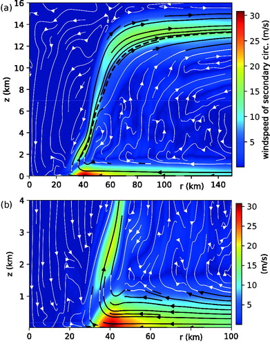
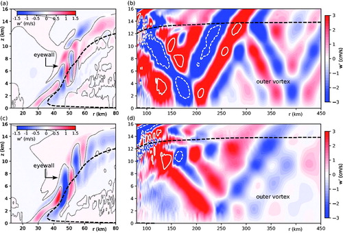
Figure 2 illustrates the secondary circulation of the basic state. The maximum wind speed ($\sqrt{u_b^2+w_b^2}=31$ m s⁻¹) of the surface inflow is relatively strong but not much greater than typical observations pertaining to major hurricanes (Zhang et al., 2011). The inflow intensity is greatest slightly outward of the corner flow region, where the streamlines rapidly turn upward into the eyewall cloud. Note that the azimuthal vorticity associated with the secondary circulation in the vicinity of the corner flow (Fig. 1e) is comparable in magnitude to the peak vertical and radial vorticities associated with the primary circulation. Note also that the streamline associated with the deep updraft and outflow passing through the location of v_bm is virtually congruent with the principal AM isoline. Such a condition is to be expected for a nearly equilibrated axisymmetric vortex. As usual, the secondary circulation in the eye is dominated by weak subsidence. The streamlines are somewhat less coherent at larger radii between the surface inflow and upper tropospheric outflow. Concerns that such incoherence may indicate a significant departure from equilibrium are alleviated by noting that the regional wind speeds are minute compared to peak values.

Fig. 2. The secondary circulation of the basic state. (a) Magnitude (colour) and streamlines of the velocity field (u_b, w_b) in the r-z plane. The streamlines are shaded white or black if the magnitude of the local velocity vector is respectively less than or greater than 5 m s⁻¹. The dashed black curve is the principal AM isoline. (b) Magnified view of the secondary circulation in (a) in the lower troposphere.

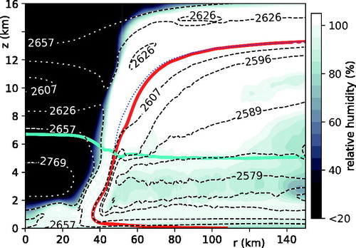
Figure 3 illustrates the moist-thermodynamic structure of the basic state. Contours of saturated pseudoadiabatic entropy ($s_{p*}$) are shown superimposed on the relative humidity distribution. Relative humidity is calculated with respect to liquid water if the absolute temperature satisfies $T>T_0\equiv 273.15$ K, but is otherwise calculated with respect to ice. It should come as no surprise that the eyewall and outflow regions are predominantly saturated or slightly supersaturated. The dashed black-and-white contours correspond to $s_{p*}$ for liquid-only condensate (Bryan, 2008). It is seen that the angular momentum and liquid-only $s_{p*}$ contours passing through the location of v_bm are congruent as they ascend along the eyewall up to the freezing level. At higher altitudes, the angular momentum contour appears to stay closer to the dotted-blue $s_{p*}$ contour calculated under the assumption of ice-only condensate (Hakim, 2011). The preceding observations suggest that the eyewall updraft region is in a state of approximate slantwise convective neutrality with respect to appropriately defined pseudoadiabatic thermodynamics. Such a state of affairs is consistent with the classical steady state theory expounded by Emanuel (1986).

Fig. 3. The moist-thermodynamic structure of the basic state, illustrated primarily by the distributions of relative humidity (shading) and $s_{p*}$ for liquid-only condensate (dashed black-and-white contours; J kg⁻¹ K^–1). The dotted blue curve is a selected contour of $s_{p*}$ computed under the assumption of ice-only condensate. The red curve is the principal AM isoline. The cyan curve traces the freezing/melting level across the vortex.

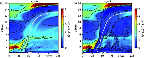
The cloud structure of the basic state is important to the linear model insofar as it determines the proportionality between $S_{\theta }^{\prime }$ and $w\prime$ in the local parameterisation of diabatic processes given by Equation (9(9a) $$\begin{array}{cc}\hfill & S{\prime }_{\theta }={\tilde{\chi }}_b{\partial }_z{\theta }_{\rho b}w\prime \hfill \\ \to \hfill & S_{\theta n}={\tilde{\chi }}_b{\partial }_z{\theta }_{\rho b}{w}_n.\hfill \end{array}$$(9a) b). When the aforementioned parameterisation is activated, there are two terms proportional to w_n on the right-hand side of Equation (3(3a) $$\begin{array}{l}\frac{\partial u_n}{\partial t}=-\frac{\partial u_b{u}_n}{\partial r}-in{\Omega }_b{u}_n-w_b\frac{\partial u_n}{\partial z}+{\xi }_b{v}_n-\frac{\partial u_b}{\partial z}{w}_n\\ -c_{pd}\frac{\partial {\Pi }_b}{\partial r}{\theta }_{\rho n}-\mu {\theta }_{\rho b}\frac{\partial }{\partial r}\left[\frac{{\Pi }_b}{{\theta }_{\rho b}}{\theta }_{\rho n}+\frac{{\Pi }_b}{{\rho }_b}{\rho }_n\right]+{\tilde{D}}_{un}\end{array}$$(3a) d) that may be unified as follows: (28a) $$-\frac{\partial {\theta }_{\rho b}}{\partial z}{w}_n+S_{\theta n}\to -\frac{{\theta }_{\rho b}}{g}{\tilde{N}}^2{w}_n,$$(28a) in which (28b) $${\tilde{N}}^2\equiv \left(1-{ϵ}_{\chi }{\tilde{\chi }}_b\right)\frac{g}{{\theta }_{\rho b}}\frac{\partial {\theta }_{\rho b}}{\partial z}.$$(28b) A typical value of ${ϵ}_{\chi }{\tilde{\chi }}_b$ between zero and one reduces ${\tilde{N}}^2$ and thereby diminishes the negative/positive Eulerian change in ${\theta }_{\rho }$ associated with a perturbative updraft/downdraft. While not precisely the conventionally defined moist static stability, ${\tilde{N}}^2$ has a similar significance. Figure 4 compares the distribution of ${\tilde{N}}^2$ in the approximate dry limit (${ϵ}_{\chi }=0$) to the moist variant with ${ϵ}_{\chi }=1$. It is seen that incorporating the cloud coverage of the basic state reduces ${\tilde{N}}^2$ up to an order of magnitude in the eyewall updraft. Significant reduction is also found over much of the depicted area within and underneath the upper outflow of the tropical cyclone. By contrast, ${\tilde{N}}^2$ exhibits minimal change in the virtually cloud-free region of the eye situated above the boundary layer.

Fig. 4. Distributions of ${\tilde{N}}^2$ for (a) ${ϵ}_{\chi }=0$ and (b) ${ϵ}_{\chi }=1$. The dashed white curves in (a) and (b) correspond to the principal AM isoline.

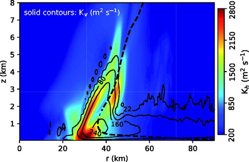
As explained earlier, the eddy diffusivities used by the linear model are linked to those regulating the basic state. Figure 5 shows the eddy diffusivities that are defined by Equation (16)(16) $$K_{h/v}^m=\max \left({ϵ}_k{K}_{h/v,\text{sm}}^m,K_{h/v,\text{min}}^m\right),$$(16) with ${ϵ}_k=1$. Choosing ${ϵ}_k=1$ lets $K_{h/v}^m=K_{h/v,\text{sm}}^m$ throughout much of the inner core. The maximum values are somewhat large but have orders of magnitude consistent with those inferred from observations (Zhang and Montgomery, 2012; Rogers et al., 2013). To reduce the potential for spurious or uninteresting small-scale instabilities where the eddy diffusivities in the CM1 simulation are exceptionally small, the lower limits $K_{h,\text{min}}^m=200$ m² s⁻¹ and $K_{v,\text{min}}^m=20$ m² s⁻¹ are imposed on the distributions.

Fig. 5. Horizontal (colour) and vertical (solid contours) momentum eddy diffusivities in the middle-to-lower tropospheric core of the simulated tropical cyclone. The dashed curve is the principal AM isoline.

5. Linear instability analysis of a mature tropical cyclone

The present section of this article examines the instability of the tropical cyclone described in Section 4. The primary objective is to elucidate the dependence of the dominant instability mode on the parameterisation of the perturbation of diabatic forcing. Sensitivity to the parameterisation of small-scale turbulence is also addressed. The analysis concludes with an assessment of the relevance of 2D instability theory.

A few preliminary remarks are warranted. Henceforth, the meaning of $F\prime$ is subtly changed from the exact difference $F-F_b$ to the first-order perturbation of the generic field F obtained from the linear model [Equations (3a)–(3e); Equation (20)(20) $$\frac{d{\mathbf{x}}_n}{dt}={\mathbf{M}}_n{\mathbf{x}}_n,$$(20) ]. The new meaning of $F\prime$ applies to both figures and text. Moreover, the amplitudes of displayed instability modes are invariably chosen to render the maximum value of $v\prime$ ($2\left|v_n\right|$) equal to one-tenth of v_bm. The preceding convention amounts to letting $\left|a_{\lambda }\right|=0.1v_{bm}/\left|2V_{\lambda }{e}^{{\lambda }_R{t}_s}\right|$, in which $V_{\lambda }$ is the azimuthal velocity element of ${\mathbf{X}}_{\lambda }$ with the greatest magnitude, and t_s is the time of the snapshot. In some cases, the second-order change to the mean vortex (${\mathbf{x}}_0$) that will have attended the creation of such a state from a weaker disturbance by way of Equation (24(24a) $$\frac{d{\mathbf{x}}_0}{dt}-{\mathbf{M}}_0{\mathbf{x}}_0={\mathbf{\beta }}_{\lambda }{e}^{2{\lambda }_{R}t},$$(24a) a) is found to have winds moderately stronger than $v\prime$ in certain areas of the flow. Such a result indicates that the arbitrarily chosen mode amplitude is slightly beyond the threshold for the quantitative accuracy of Equation (24(24a) $$\frac{d{\mathbf{x}}_0}{dt}-{\mathbf{M}}_0{\mathbf{x}}_0={\mathbf{\beta }}_{\lambda }{e}^{2{\lambda }_{R}t},$$(24a) a). Choosing a smaller amplitude for rigorous compliance with the assumptions of our theoretical framework would not change forthcoming depictions of the spatial structure of ${\mathbf{x}}_0$ or the dependent kinetic energy perturbation $\delta \text{KE}$ defined later.

Finally, although the physics parameterisations are varied, the domain size and peripheral sponge-layer of the linear model used to find the instability modes do not change from one calculation to the next. As in the CM1 simulation used to generate the basic state, the invariant domain of the linear model extends radially to $r_B=1061.25$ km and vertically to $z_B=29.5$ km. The sponge damping coefficient is given by $\gamma =\{2+\tanh [(r-r_{\gamma })/\delta r_{\gamma }]+\tanh [(z-z_{\gamma })/\delta z_{\gamma }]\}/2{\tau }_{\gamma }$, in which $r_{\gamma }=961.25$ km, $\delta r_{\gamma }=z_{\gamma }=25$ km, $\delta z_{\gamma }=0.75$ km and ${\tau }_{\gamma }=300$ s. Further computational details are provided in due course.

5.1. Sensitivity to the parameterisation of diabatic forcing

The dominant instability of the tropical cyclone under consideration is sensitive to the degree of diabatic forcing allowed in the linear model. The sensitivity is illustrated below by adjusting ${ϵ}_{\chi }$ in Equation (9(9a) $$\begin{array}{cc}\hfill & S{\prime }_{\theta }={\tilde{\chi }}_b{\partial }_z{\theta }_{\rho b}w\prime \hfill \\ \to \hfill & S_{\theta n}={\tilde{\chi }}_b{\partial }_z{\theta }_{\rho b}{w}_n.\hfill \end{array}$$(9a) b) for $S_{\theta n}$ while keeping turbulent transport consistently parameterized with ${ϵ}_k=1$. A value of the diabatic forcing parameter (${ϵ}_{\chi }$) in the neighbourhood of unity has some basic credibility (Section 2.2) but may not coincide with the best representation of reality. A smaller value between 0 and 1 seems plausible if, say, the eyewall were to become nonuniformly saturated around an azimuthal circuit. Values of ${ϵ}_{\chi }$ very close to 0 or appreciably greater than 1 seem difficult to justify on physical grounds, but are of theoretical interest.

The present method for computing the primary instability modes of the vortex follows the general procedure outlined in Section 3.2. The most unstable eigenmode (MUM) for a given ${ϵ}_{\chi }$ and azimuthal wavenumber n is provisionally equated to that which dominates a perturbation within 1 day of initialising the linear model [Equations (3a)–(3e)] with random noise in ${\theta }_{\rho }^{\prime }$. The absolute MUM (AMUM) is defined to be that which possesses the largest growth rate for all n in the closed interval between 0 and 8. The time integration is conducted on a grid (set of staggered grids) with double the resolution of the CM1 simulation that generated the basic state. The aforementioned grid is denoted G2 and holds $N_t=733,184$ values of the prognostic perturbation fields. All MUMs are confirmed to be solutions of the eigenproblem on a second grid (G4) with quadruple the resolution of the CM1 grid (G1). All eigenfrequencies and eigenfunctions shown in Section 5 of this paper are taken from the G4 solutions. For those interested, Appendix C discusses convergence of numerical results with increasing resolution.

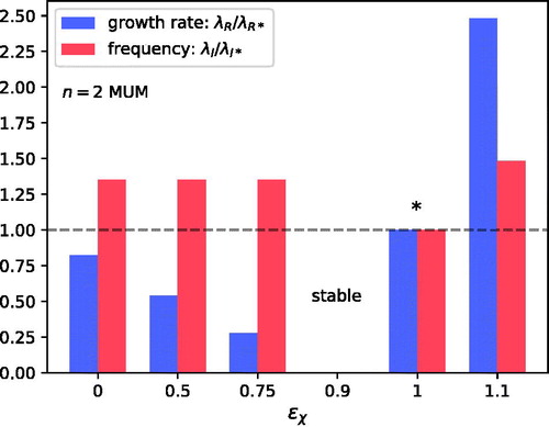
Extensive computations reveal that the AMUM corresponds to n = 2 for ${ϵ}_{\chi }\in \{0,0.5,1\}$. Despite its common dominance, the n = 2 MUM varies considerably with the allowed degree of diabatic forcing measured by ${ϵ}_{\chi }$. Figure 6 shows the variation of the complex eigenfrequency λ. The growth rate (λ_R) gradually decays with increasing ${ϵ}_{\chi }$ until apparently vanishing at 0.9. By contrast, the oscillation frequency (λ_I) changes little. The preceding behaviour is similar to that reported by SM07 for the n = 3 MUM of a cloudy vortex resembling a category-3 hurricane with no mean secondary circulation. On the other hand, increasing ${ϵ}_{\chi }$ from 0.9 to 1 introduces a new mode of instability that oscillates slower and grows faster than any of its predecessors. Further amplification of ${ϵ}_{\chi }$ to 1.1 substantially increases both λ_R and $\left|{\lambda }_I\right|$. One might reasonably speculate that high sensitivity to variation of ${ϵ}_{\chi }$ in the neighbourhood of unity is related to approximate slantwise convective neutrality with respect to pseudoadiabatic thermodynamics in the eyewall (Fig. 3).

Fig. 6. Complex eigenfrequency λ of the n = 2 MUM of the simulated tropical cyclone of Section 4 versus the diabatic forcing parameter ${ϵ}_{\chi }$. The real (blue) and imaginary (red) parts of the eigenfrequency are normalised to their respective values (${\lambda }_{R*}=7.89\times {10}^{-5}$ s⁻¹ and ${\lambda }_{I*}=-1.30\times {10}^{-3}$ s⁻¹) obtained for ${ϵ}_{\chi }=1$. The absence of a discernible instability precludes the plotting of data for ${ϵ}_{\chi }=0.9$. Note that the positive ratio ${\lambda }_I/{\lambda }_{I*}$ represents a nondimensional magnitude of the oscillation frequency; the actual value of λ_I is negative. All results depicted here and in Figs. 7–12 are for systems in which turbulent transport is parameterized with ${ϵ}_k=1$.

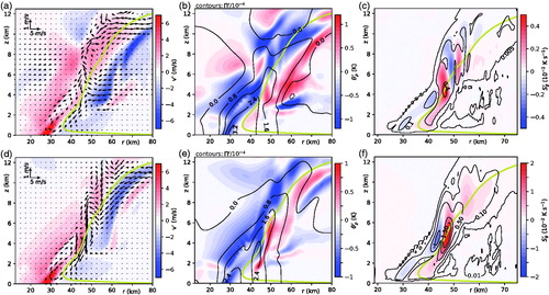
Figure 7 shows the basic inner-core structure of the n = 2 MUM for values of the diabatic forcing parameter below (${ϵ}_{\chi }=0.5$) and above (${ϵ}_{\chi }=1$) the apparent stability point. The left column shows selected views of the asymmetric velocity perturbation. The middle column illustrates the thermal structure of each mode in terms of ${\theta }_{\rho }^{\prime }$ and $\Pi \prime$. The right column shows the distributions of diabatic forcing. The velocity perturbations of the two modes are qualitatively similar near the surface but clearly differ aloft. Whereas the pressure perturbations seem only subtly distinct, disparities in ${\theta }_{\rho }^{\prime }$ are pronounced. Marked distinctions in the perturbations of the secondary circulation and potential temperature in the middle and upper troposphere coincide with substantial differences in $S_{\theta }^{\prime }$. Not only does $S_{\theta }^{\prime }$ have a greater amplitude in the MUM corresponding to ${ϵ}_{\chi }=1$, but the two spatial patterns diverge considerably above 4 km in the eyewall updraft region of the vortex.

Fig. 7. (a)–(c) Basic inner-core structure of the n = 2 MUM for ${ϵ}_{\chi }=0.5$. (a) Vertical slices of the velocity perturbations in the azimuthal direction (colour) and in the r-z plane (vectors). (b) Vertical slices of the perturbations of density potential temperature (colour) and the Exner function (contours). (c) Vertical slice of the perturbation to diabatic forcing (colour) and contours of its maximum value along an azimuthal circuit. (d)–(f) As in (a)–(c) but for ${ϵ}_{\chi }=1$. The yellow curve in each plot is the principal AM isoline. The slices in (a, b, d, e) are at an azimuth where $v\prime$ is maximised. The colour slices in (c) and (f) are at an azimuth where $S_{\theta }^{\prime }$ is maximised.

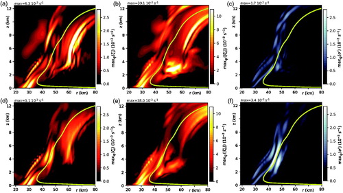
Figure 8 elaborates on the inner-core structure of each MUM. The left column shows the intensity of the vertical vorticity perturbation ${\zeta }_z^{\prime }$, as measured by its maximum value over $\phi$. In each MUM, the intensity peaks of ${\zeta }_z^{\prime }$ roughly coincide with a subset of regions where the radial gradient of basic state potential vorticity is locally enhanced (see Fig. 1c). The amplitudes of the peaks differ considerably between the two modes, especially in the middle-to-upper troposphere. The middle column depicts the maximum magnitude of the horizontal vorticity perturbation ${\mathbf{\zeta }}_h^{\prime }$ along an azimuthal circuit. In both MUMs, $\left|{\mathbf{\zeta }}_h^{\prime }\right|$ broadly exceeds the vertical vorticity perturbation. As before, differences between the two MUMs are mainly seen in the amplitudes of various peaks of the plotted field. The right column shows the circuit-maximum of the horizontal divergence, defined by $\sigma \prime \equiv \left[{\partial }_r(ru\prime )+{\partial }_{\phi }v\prime \right]/r$. In both MUMs, $\sigma \prime$ is broadly smaller than the vertical vorticity perturbation near the surface, but is far from negligible. In the middle tropospheric region of the eyewall cloud, the amplitudes of $\sigma \prime$ and ${\zeta }_z^{\prime }$ are comparable to each other. The MUM corresponding to ${ϵ}_{\chi }=1$ is distinguished by having a middle tropospheric peak of $\sigma \prime$ that slightly exceeds the inner core maximum of ${\zeta }_z^{\prime }$.

Fig. 8. (a)–(c) Maximum values over $\phi$ (${\max }_{\phi }$) of (a) the vertical vorticity perturbation, (b) the magnitude of the horizontal vorticity perturbation, and (c) the divergence of the horizontal velocity perturbation of the n = 2 MUM for ${ϵ}_{\chi }=0.5$. (d)–(f) As in (a)–(c) but for ${ϵ}_{\chi }=1$. The yellow curve in each plot is the principal AM isoline.

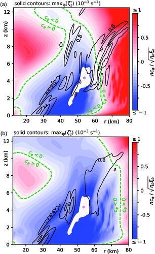
Figure 9 illustrates for each MUM how the azimuthal phase velocity minus the local angular velocity of the primary circulation ($c_{\phi }\equiv -{\lambda }_I/n-{\Omega }_b$) varies over the core of the tropical cyclone. The dashed green curves representing the zero contours of $c_{\phi }$ correspond to where the mode corotates with the mean flow. Negative/positive values of $c_{\phi }$ indicate locally retrograde/prograde wave propagation in the azimuthal direction. The superimposed vertical vorticity distribution (solid black contours) of the MUM corresponding to ${ϵ}_{\chi }=1$ is concentrated in the region of retrograde propagation. On the other hand, the MUM with weaker diabatic forcing has a middle-to-upper tropospheric swath of intense ${\zeta }_z^{\prime }$ that extends well into the region of prograde propagation. In both cases, the magnitude of the intrinsic frequency of the mode ($n{c}_{\phi }$) is less than the nominal inertial frequency ($\sqrt{{\eta }_b{\xi }_b}$) where the vorticity anomalies are peaked. While notable, such local slowness does not necessarily indicate that traditional asymmetric balance theory (Shapiro and Montgomery, 1993) would provide an accurate description of the wave dynamics. Bear in mind that the issue is complicated by the moist secondary circulation and the vertical shear in v_b. Moreover, even small deviations from balanced dynamics are potentially important to the instability mechanism.

Fig. 9. (a) Intrinsic frequency $n{c}_{\phi }$ of the n = 2 MUM normalised to the nominal inertial frequency $\sqrt{{\eta }_b{\xi }_b}$ for the case in which ${ϵ}_{\chi }=0.5$. The dashed green contours show where the intrinsic frequency is zero. The white area marked with an asterisk coincides with a region where ${\eta }_b{\xi }_b<0$ and the normalisation frequency is imaginary. The solid black contours of the amplitude (maximum over $\phi$) of ${\zeta }_z^{\prime }$ are shown for reference. (b) As in (a) but for ${ϵ}_{\chi }=1$.

Moving outward to where r exceeds 100 km, the MUMs acquire intrinsic frequencies that broadly satisfy ${\eta }_b{\xi }_b\ll {(n{c}_{\phi })}^2\ll {\tilde{N}}^2$ (not shown). The preceding condition suggests that the intrinsic frequency lies comfortably within the regime of inertia-gravity waves. Consistent with such waves, one finds that $\left|{\zeta }_{zn}\right|\ll \left|{\sigma }_n\right|$ beyond the core of the vortex, barring sporadic pockets of violation. The right panels in Fig. 10 convey the basic structure of the outer waves as represented by $w\prime$ in the two MUMs under consideration. Although both modes are normalised to have the same inner core maximum value of $v\prime$, the outer waves have appreciably stronger vertical velocities for the case in which ${ϵ}_{\chi }=0.5$. Whether such a distinction is relevant to the mechanism of modal growth is a question left for future analysis. In theory, seemingly weak inertia-gravity wave radiation may contribute significantly to the prevailing low-n instability of an intense tropical cyclone (Menelaou et al., 2016; Schecter and Menelaou, 2017). However, the author is unaware of any existing method for assessing the importance of inertia-gravity wave emission to the growth of a multifaceted instability mode of a convective vortex with the geometrical complexity of a realistic hurricane.

Fig. 10. (a, b) Slices of the vertical velocity perturbation of the n = 2 MUM in (a) the inner core and (b) the outer region of the vortex for the case in which ${ϵ}_{\chi }=0.5$. The dotted black contours in (a) correspond to $w\prime =0$. The solid (dashed) white contours in (b) correspond to $w\prime =7$ (−7) cm s⁻¹. Note that the units of the colorbar labels differ between (a) and (b). (c, d) As in (a, b) but for ${ϵ}_{\chi }=1$. In all plots, the dashed black contour corresponds to the principal AM isoline. The azimuth of the top (bottom) row of the figure is equivalent to that of Fig. 7a (7d).

Figures 11a,d show changes to the mean flow that attend the growth of each instability mode from an asymptotically small disturbance. The symmetric component of the perturbation is given by ${\mathbf{x}}_0={\mathbf{X}}_p{e}^{2{\lambda }_R{t}_s}$, with X_p given by Equation (24(24a) $$\frac{d{\mathbf{x}}_0}{dt}-{\mathbf{M}}_0{\mathbf{x}}_0={\mathbf{\beta }}_{\lambda }{e}^{2{\lambda }_{R}t},$$(24a) d). The growth of either instability mode modestly reduces the $\phi$-averaged azimuthal wind speed at the initial location of maximal intensity while accelerating the cyclonic rotation of the inner eye, at least in the lower troposphere. The middle tropospheric patterns of symmetric azimuthal acceleration and deceleration are clearly dissimilar inward of the principal AM isoline. Moreover, the MUM affected by weaker diabatic forcing (${ϵ}_{\chi }=0.5$) induces greater positive and negative azimuthal accelerations of the mean flow in the upper-outer part of the eyewall updraft. The perturbation of the symmetric secondary circulation $(u_0,w_0$) that emerges during the growth of either instability mode notably includes a band of eddies along the eyewall updraft. The bands associated with the two MUMs are distinguishable in part by having opposite rotational tendencies at various locations.

Fig. 11. (a) The symmetric velocity perturbation that attends the growth of the n = 2 MUM for the case in which ${ϵ}_{\chi }=0.5$. Colours depict v₀ whereas vectors depict (u₀, w₀). (b) The perturbation of kinetic energy density associated with the n = 2 MUM and the attendant symmetric modification of the vortex for the case in which ${ϵ}_{\chi }=0.5$. The perturbation is expressed as a positive or negative percentage of the local kinetic energy density of the basic state. The dotted black contours correspond to $\delta \text{KE}=0$. (c) The distribution of ${\text{KE}}_n$ associated with the n = 2 MUM for the case in which ${ϵ}_{\chi }=0.5$. The white and black contours correspond to ${\text{KE}}_n=[0.6,3.2,6.3,13,19]$ J m⁻³. (d)–(f) As in (a)–(c) but for ${ϵ}_{\chi }=1$. The yellow or red curve in each plot is the principal AM isoline. The thick black or blue line drawn from the location of v_bm to the surface [in all plots but (b) and (e)] shows where v_b is maximised with respect to variation of r in the boundary layer. The thin black curves in (a) and (d) trace the edges of the unperturbed eyewall updraft, where w_b is 2.5% of its maximum positive value.

Figures 11b,e show the perturbation of kinetic energy density $\delta \text{KE}$ associated with the growth of each MUM. To second-order in the asymmetric mode amplitude, (29) $$\begin{array}{cc}\delta \text{KE}\hfill & \equiv \overline{\frac{\rho }{2}\left(u^2+v^2+w^2\right)}-\frac{{\rho }_b}{2}\left(u_b^2+v_b^2+w_b^2\right)\hfill \\ \hfill & ={\rho }_b\left(u_b{u}_0+v_b{v}_0+w_b{w}_0\right)+{\rho }_b\left(|u_n{|}^2+|v_n{|}^2+|w_n{|}^2\right)\hfill \\ \hfill & +\frac{{\rho }_0}{2}\left(u_b^2+v_b^2+w_b^2\right)+2\mathfrak{R}\left[\left(u_b{u}_n+v_b{v}_n+w_b{w}_n\right){\rho }_n^{*}\right],\hfill \end{array}$$(29) in which the overline denotes an azimuthal average. It has been verified that the bottom line in the second equality involving the density perturbation is negligible (not shown). Moreover, it is seen that the distribution of $\delta \text{KE}$ — here divided by ${\text{KE}}_b\equiv {\rho }_b(u_b^2+v_b^2+w_b^2)/2$ —is similar to that of v₀ regardless of whether ${ϵ}_{\chi }$ is 0.5 or 1.

The contribution to $\delta \text{KE}$ from the asymmetric fields is well approximated by the following positive definite measure of local wave intensity: ${\text{KE}}_n\equiv {\rho }_b(|u_n{|}^2+|v_n{|}^2+|w_n{|}^2)$. Figures 11c,f show the spatial distributions of ${\text{KE}}_n$ for the two MUMs under present consideration. Both MUMs have their greatest values of ${\text{KE}}_n$ near the surface, inward of the radius of maximum wind, in the vicinity of where the vertical vorticity of the basic state (ζ_zb) has a pronounced maximum. The middle-to-upper tropospheric peaks of ${\text{KE}}_n$ are found in distinct locations. Above the surface perturbation, the distribution of ${\text{KE}}_n$ corresponding to ${ϵ}_{\chi }=0.5$ has relatively strong peaks outward of the central part of the eyewall. The instability mode that results from allowing greater diabatic forcing (${ϵ}_{\chi }=1$) has its principal middle tropospheric maximum of ${\text{KE}}_n$ well within the eyewall updraft.

Differences between the MUMs are also evident in various terms that formally contribute to the growth rate of ${\text{KE}}_n$. Equations (3a)–(3c) imply that (30a) $$\frac{\partial {\text{KE}}_n}{\partial t}=\text{PC}+\text{SC}+\text{BNC}+\text{AFX}+\text{PFX}+\text{TRB},$$(30a) in which (30b) $$\text{PC}\equiv -2{\rho }_{b}r\frac{\partial {\Omega }_b}{\partial r}\mathfrak{R}\left[u_n{v}_n^{*}\right]-2{\rho }_b\frac{\partial v_b}{\partial z}\mathfrak{R}\left[w_n{v}_n^{*}\right],$$(30b) (30c) $$\begin{array}{l}\text{SC}\equiv -2{\rho }_b\frac{\partial u_b}{\partial r}{\left|u_n\right|}^2-2{\rho }_b\frac{u_b}{r}{\left|v_n\right|}^2-2{\rho }_b\frac{\partial w_b}{\partial z}{\left|w_n\right|}^2\\ -2{\rho }_b\left(\frac{\partial u_b}{\partial z}+\frac{\partial w_b}{\partial r}\right)\mathfrak{R}\left[u_n{w}_n^{\ast }\right],\end{array}$$(30c) (30d) $$\text{BNC}\equiv \frac{2{\rho }_b\tilde{g}}{{\theta }_{\rho ba}}\mathfrak{R}\left[w_n{\theta }_{\rho n}^{*}\right]-2c_{pd}{\rho }_b\frac{\partial {\Pi }_b}{\partial r}\mathfrak{R}\left[u_n{\theta }_{\rho n}^{*}\right],$$(30d) (30e) $$\text{AFX}\equiv -\frac{1}{r}\frac{\partial \left(r{u}_b{\text{KE}}_n\right)}{\partial r}-\frac{\partial \left(w_b{\text{KE}}_n\right)}{\partial z}+\frac{{\text{KE}}_n}{{\rho }_b}\left[\frac{1}{r}\frac{\partial \left(r{\rho }_b{u}_b\right)}{\partial r}+\frac{\partial \left({\rho }_b{w}_b\right)}{\partial z}\right],$$(30e) (30f) $$\begin{array}{cc}\text{PFX}\equiv \hfill & -\frac{2c_{pd}}{r}\frac{\partial \left\{r{\rho }_b{\theta }_{\rho b}\mathfrak{R}\left[u_n{\check{\Pi }}_n^{*}\right]\right\}}{\partial r}-2c_{pd}\frac{\partial \left\{{\rho }_b{\theta }_{\rho b}\mathfrak{R}\left[w_n{\check{\Pi }}_n^{*}\right]\right\}}{\partial z}\hfill \\ \hfill & \hfill \\ \hfill & +2c_{pd}\mathfrak{R}\left\{\left[\frac{1}{r}\frac{\partial \left(r{\rho }_b{\theta }_{\rho b}{u}_n\right)}{\partial r}+\frac{in{\rho }_b{\theta }_{\rho b}{v}_n}{r}+\frac{\partial \left({\rho }_b{\theta }_{\rho b}{w}_n\right)}{\partial z}\right]{\check{\Pi }}_n^{*}\right\},\hfill \end{array}$$(30f) (30g) $$\text{TRB}\equiv 2{\rho }_b\mathfrak{R}\left[u_n{\tilde{D}}_{un}^{*}+v_n{\tilde{D}}_{vn}^{*}+w_n{\tilde{D}}_{wn}^{*}\right].$$(30g) The term labelled PC combines tendencies proportional to the radial and vertical shear of the primary circulation of the basic state. SC combines tendencies proportional to u_b and the spatial derivatives of the velocity fields of the secondary circulation. BNC is linked to the vertical and radial buoyancy accelerations. AFX primarily represents the convergence of the advective flux of ${\text{KE}}_n$. The included correction is attributable to the small but nonzero divergence of the momentum density of the basic state. PFX primarily represents the convergence of the flux vector associated with forcing by the perturbation of the pressure-gradient. The included correction is attributable to the small but nonzero divergence of the approximate momentum perturbation weighted by ${\theta }_{\rho b}$. TRB is associated with turbulent momentum transport and (to a lesser extent) sponge-damping near the upper and outer edges of the computational domain. It is worth pointing out that substantial cancellations of the tendency terms often result in a local value of ${\partial }_t{\text{KE}}_n=2{\lambda }_R{\text{KE}}_n$ that is much smaller than its individual parts.

Figure 12 illustrates how the value of the diabatic forcing parameter (${ϵ}_{\chi }$) affects the volume-integrals of the ${\text{KE}}_n$ tendency terms pertaining to the n = 2 MUM of the tropical cyclone. The volume integrals are over the entire domain of the linear model. The results are similar for all ${ϵ}_{\chi }\le 0.75$. The integral of PC provides the greatest positive contribution to the sum. The component of PC associated with the radial shear of the basic state is dominant. The integral of SC is smaller than that of PC, but often greater than the integral of all terms combined. The integrals of both BNC and TRB are negative and substantial. On the other hand, the integrals of AFX, PFX and their displayed sum are negligible. The budget corresponding to ${ϵ}_{\chi }=1$ has several distinctive features. The difference between the PC and SC integrals is appreciably reduced. Moreover, the BNC integral is positive. Of lesser significance, the combined integral of AFX and PFX is discernibly negative owing mostly to the corrective component of PFX. Increasing ${ϵ}_{\chi }$ to 1.1 moves the strongest peaks of the asymmetric kinetic energy density from the surface to the middle troposphere (not shown). The attendant structural change coincides with notable modifications to the global ${\text{KE}}_n$-budget. For example, the vertical shear component of the PC integral becomes dominant. Moreover, the integral of BNC becomes nearly equal to that of PC.

Fig. 12. Domain integrals of the individual contributions to ${\partial }_t{\text{KE}}_n$ [Equations (30b)–(30g)] and their sum for the n = 2 MUM with (left to right) ${ϵ}_{\chi }=0$ to 1.1. The value of each integral is normalised to that of ${\partial }_t{\text{KE}}_n$. The contributions from AFX and PFX are combined into APFX. The PC contribution is decomposed into the radial shear component proportional to ${\partial }_r{\Omega }_b$ (r, dark red) and the vertical shear component proportional to ${\partial }_z{v}_b$ (v, light red). The TRB contribution is decomposed into the primary part attributable to turbulent dissipation (dark cyan) and the much smaller part attributable to sponge damping (light cyan cap).

5.2. Sensitivity to the parameterisation of turbulent transport

The MUM associated with arbitrary n generally varies with the parameterisation of small-scale turbulence. Sensitivity to the intensity of turbulent transport is illustrated herein by reducing the value of ${ϵ}_k$ defined in Section 2.3. The minimum value of ${ϵ}_k$ to be considered will be 0.0625, which is slightly below the limit of 0.07 (0.08) that guarantees $K_h^m$ ($K_v^m$) will uniformly equal the value specified for $K_{h,\text{min}}^m$ ($K_{v,\text{min}}^m$) in Section 4.

Figure 13 shows how reducing ${ϵ}_k$ affects the complex eigenfrequencies of the MUM and the second most unstable eigenmode (SMUM) of linear systems with n = 2 and ${ϵ}_{\chi }\in \{0.5,1\}$. Results are shown for ${ϵ}_k=1$, 0.25 and 0.0625. As before, the MUM is provisionally equated to the prevailing instability mode that emerges during a time integration of the linear model initialised with a random distribution of ${\theta }_{\rho }^{\prime }$ on G2. The SMUM is provisionally equated to the prevailing instability mode of a continued integration that filters out the MUM [see Equation (26)(26) $${\mathbf{x}}_n(t=0)=\mathbf{Y}-\sum _{\alpha <\beta }\frac{〈{\mathbf{X}}_{{\lambda }^{(\alpha )}}^L,\mathbf{Y}〉}{〈{\mathbf{X}}_{{\lambda }^{(\alpha )}}^L,{\mathbf{X}}_{{\lambda }^{(\alpha )}}〉}{\mathbf{X}}_{{\lambda }^{(\alpha )}},$$(26) ]. Both modes are verified to solve the eigenproblem on G4. The displayed data are obtained from the G4 eigensolutions.

Fig. 13. Variation of the complex eigenfrequency λ of the n = 2 MUM and SMUM with the small-scale turbulence parameter ${ϵ}_k$ for systems with (top) ${ϵ}_{\chi }=0.5$ and (bottom) ${ϵ}_{\chi }=1$. The real (blue) and imaginary (red) parts of each eigenfrequency are normalised to their respective values (${\lambda }_{R*}=7.89\times {10}^{-5}$ s⁻¹ and ${\lambda }_{I*}=-1.30\times {10}^{-3}$ s⁻¹) obtained for the MUM when ${ϵ}_{\chi }={ϵ}_k=1$.

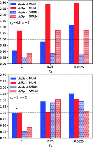
Consider first the group of linear systems that allow a medium degree of diabatic forcing (${ϵ}_{\chi }=0.5$). Section 5.1 thoroughly described the dominant MUM when ${ϵ}_k=1$. The corresponding SMUM has a lower oscillation frequency and is structurally distinct in having KE_n concentrated in the middle troposphere (not shown). Reducing ${ϵ}_k$ introduces a faster instability that overtakes both of the aforementioned eigenmodes. The greater growth rate (λ_R) of the new MUM coincides with a greater oscillation frequency ($\left|{\lambda }_I\right|$). The new MUM is also structurally distinct in having KE_n largely confined to a shallow layer near the surface (Fig. 14a). Moreover, the global KE_n budget is distinguished from that of the original MUM by having a greater vertical shear component of PC, and a minimal contribution from SC (Fig. 14b).

Fig. 14. (a) Spatial distribution of ${\partial }_t{\text{KE}}_n=2{\lambda }_R{\text{KE}}_n$ for the n = 2 MUM with ${ϵ}_{\chi }=0.5$ and ${ϵ}_k=0.0625$. The white and black contours correspond to ${\partial }_t{\text{KE}}_n=[0.1,0.5,1.0,2.0,4.0]$ ${10}^{-3}$ W m⁻³. (b) Domain integrals of the individual contributions to ${\partial }_t{\text{KE}}_n$ for the n = 2 MUM with ${ϵ}_{\chi }=0.5$ and ${ϵ}_k=0.0625$. (c, d) As in (a, b) but for ${ϵ}_{\chi }=1$ and ${ϵ}_k=0.0625$. (e, f) As in (a, b) but for the n = 3 MUM with ${ϵ}_{\chi }=1$ and ${ϵ}_k=0.25$. The red curves in (a, c, e) correspond to the principal AM isoline; the dashed green curves show where $c_{\phi }=0$; the blue lines show where v_b is maximised with respect to variation of r in the boundary layer. The plots in (b, d, f) are completely analogous to those in Fig. 12.

Consider next the set of linear systems that allow relatively strong diabatic forcing (${ϵ}_{\chi }=1$). As before, the reader may consult Section 5.1 for a thorough description of the dominant MUM when ${ϵ}_k=1$. The corresponding SMUM is similar to that of the equally diffusive system with ${ϵ}_{\chi }=0.5$. Reducing ${ϵ}_k$ to 0.25 modestly accelerates the instability associated with the original MUM and leads to the appearance of a new SMUM with nearly the same growth rate. Reducing ${ϵ}_k$ to 0.0625 switches the ordering of the preceding instability modes without changing their top-tier status. The new mode is distinguished by having a greater oscillation frequency and a dissimilar distribution of KE_n above the boundary layer (Fig. 14c). Moreover, the global ${\text{KE}}_n$ budget of the new mode is distinguished by having a greater vertical shear component of PC, and a negative contribution from BNC (Fig. 14d).

It is worth remarking that decreasing the eddy diffusivity often magnifies the importance of higher wavenumber MUMs. For example, reducing ${ϵ}_k$ to 0.25 in a system with ${ϵ}_{\chi }=1$ allows an n = 3 MUM (Figs. 14e,f) to challenge its n = 2 counterpart for dominance among instability modes with substantial KE_n near the surface. While the former oscillates approximately 1.6 times faster than the latter, both MUMs have growth rates of $1.1\times {10}^{-4}$ s⁻¹.

5.3. Relationship to 2D instability theory

It is common practice to explain the instability of the primary circulation of a tropical cyclone in the context of a two-dimensional nondivergent barotropic model (see Appendix D). The foregoing analysis casts doubt on the general adequacy of such an approach. That is to say, the preceding results suggest that the three-dimensionality of the tropical cyclone under present consideration has a major impact on the prevailing mode of instability. The evidence includes MUMs with substantial horizontal vorticity and divergence. The evidence also includes major contributions from SC and/or the vertical shear component of PC to the volume integrated time-derivative of asymmetric kinetic energy (${\text{KE}}_n$).

Further insight is gained by directly comparing 2D and 3D instability theory. The 2D analysis requires reduction of the basic state to a circular shear-flow characterised by a 1 D vertical vorticity profile ${\zeta }_b(r)$. Because the asymmetric kinetic energy density of the instability usually has greatest amplitude in the lower troposphere, ζ_b will be extracted from the ρ_b-weighted vertical average of ${\zeta }_{zb}(r,z)$ (Fig. 1d) between the sea-surface and z = 2 km. The kinematic viscosity $K_{2d}$ will be varied between 0 and 4000 m²s^–1. The upper limit is roughly 1.4 times the peak value of $K_h^m$ in the 3D model when ${ϵ}_k=1$ (Fig. 5).

The nonmonotonic radial variation of ζ_b facilitates a variety of algebraic and exponential instabilities. An algebraic instability is expected to dominate the n = 1 component of an arbitrary disturbance (Smith and Rosenbluth, 1990). The exponentially growing eigenmodes associated with greater azimuthal wavenumbers are readily obtained from a complete numerical solution to the eigenproblem on a stretched radial grid comparable to that of G2. For $K_{2d}=0$, the AMUM corresponds to n = 3, but all MUMs with $2\le n\le 5$ have growth rates within 8% of the maximum (Fig. 15a). Increasing $K_{2d}$ toward 4000 m² s⁻¹ diminishes the growth rate of each MUM with greater effect at larger n; ultimately, the exponential instabilities are confined to azimuthal wavenumbers 2 and 3. The preservation of n = 3 dominance (or shared dominance) with increasing viscosity appears to be at odds with the 3D model. For ${ϵ}_k=1$ and ${ϵ}_{\chi }\in \{0,0.5,1\}$, the wavenumber-3 instability modes of the 3D model were found to be subdominant.

Fig. 15. (a) Azimuthal wavenumber (n) dependence of the growth rate of the 2D MUM for several values of $K_{2d}$, as indicated in the legend. Computed MUMs with growth rates of order ${10}^{-6}$ s⁻¹ or less (at high n and appreciable $K_{2d}$) are excluded from the plot, because they are considered virtually neutral and have questionable accuracy. (b) $K_{2d}$ dependencies of the growth rates of the two most unstable 2D eigenmodes associated with an n = 2 perturbation. (c) As in (b) but for the oscillation frequencies. The extended blue ticks on the vertical axes of (b) and (c) mark the growth rate and oscillation frequency of the n = 2 MUM of the 3D system with ${ϵ}_{\chi }=0.5$ and ${ϵ}_k=1$; the red ticks are the same but for ${ϵ}_{\chi }={ϵ}_k=1$.

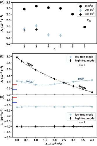
Figures 15b,c show how the complex eigenfrequencies of the two most unstable n = 2 eigenmodes vary with $K_{2d}$. The two modes are distinguished by their virtually invariant oscillation frequencies that differ roughly by a factor of 2. Decreasing the viscosity from its maximal value is seen to unleash the instability of the high-frequency mode, such that it transitions from SMUM to MUM status as $K_{2d}$ drops below 2500 m²s^–1. Despite the reordering of growth rates, neither the low-frequency mode (Fig. 16a) nor the high-frequency mode (Fig. 16b) radically changes structure with variation of $K_{2d}$ over the interval under consideration. Except for moderate radial smoothing of the vorticity wavefunction, the unshown modifications linked to greater viscosity are difficult to discern with a casual glance.

Fig. 16. (a) Vertical vorticity (red and blue), streamlines (black) and corotation circles (dashed green) of the low-frequency mode of the 2D system with $K_{2d}={10}^3$ m² s⁻¹. The streamline thickness is directly proportional to the local magnitude of the horizontal velocity perturbation $\mathbf{u}\prime$. (b) As in (a) but for the high-frequency mode. (c) As in (a) but for vertically averaged fields associated with the MUM of the 3D system with ${ϵ}_{\chi }=0.5$ and ${ϵ}_k=1$; the averaging is over a 2 km layer adjacent to the sea-surface. (d) As in (c) but with the streamlines corresponding to the irrotational component of $\mathbf{u}\prime$. (e, f) As in (c, d) but for ${ϵ}_{\chi }={ϵ}_k=1$; note that segments of the corotation circle can be found at the corners of both plots. In all subfigures, the axis labels x and y denote horizontal Cartesian coordinates measured from the center of the vortex.

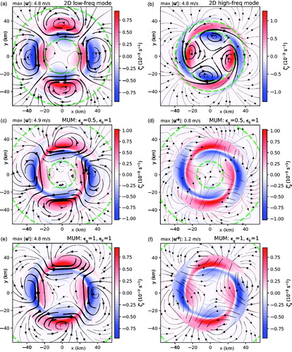
To some extent, the low-frequency mode of the 2D system that prevails under conditions of high viscosity resembles the lower tropospheric section of a typical 3D MUM that dominates under moderate diabatic forcing when turbulent transport is parameterized with ${ϵ}_k=1$. Figure 16c (16e) depicts the lower tropospheric structure of the 3D MUM corresponding to ${ϵ}_{\chi }=0.5$ (1). As in the low-frequency mode of the 2D system, the strongest perturbation eddies are centred on the outer edge of the main vorticity annulus. In similar agreement, the prominent inner and outer waves of ${\zeta }_z^{\prime }$ are close to being diametrically out of phase at azimuths where the amplitudes are peaked. On the other hand, seemingly subtle differences cannot be ignored. To begin with, the radii at which the 2D and 3D modes corotate with the circular shear flow (shown by the dashed green circles) do not coincide. In principle, even a slight displacement of a corotation radius can substantially affect the impact of locally enhanced (potential) vorticity stirring on the growth of an instability mode. The nature of any delicate imbalance of various growth and decay mechanisms may also be sensitive to small variations in the relative amplitudes and phases of the primary inner and outer vorticity waves. Moreover, the horizontal velocity perturbations associated with the depicted 3D instability modes have nonnegligible divergence. Figures 16d,f illustrate the divergent (irrotational) components of the modal flow fields obtained from a standard Helmholtz decomposition as explained in Appendix E. The maximum divergent wind speed for ${ϵ}_{\chi }=0.5$ (1) is an appreciable 16% (27%) of the maximum nondivergent wind speed.

It is notable that (for n = 2) the low-frequency instability modes of both the 2D system and the 3D systems studied in Section 5.2 are superceded by higher frequency modes as viscosity tends toward zero. The low-viscosity 3D MUM corresponding to ${ϵ}_{\chi }=0.5$ and ${ϵ}_k=0.0625$ (Fig. 14a) is fairly similar to its 2D counterpart (Fig. 16b). To begin with, the 3D MUM is confined to a shallow layer near the surface. Moreover, unshown analysis of the horizontal flow in the lower troposphere demonstrates that the strongest perturbation eddies are centred on the inner edge of the main vorticity annulus, and that a corotation radius lies in between the primary inner and outer vorticity waves. In good agreement with a key assumption of the 2D model, the maximum magnitude of the divergent component of the lower tropospheric velocity perturbation (averaged over a 2-km layer adjacent to the sea-surface) is merely 6% of the maximum nondivergent wind speed. On the other hand, the 2D model does not provide an entirely accurate picture of the low viscosity perturbation dynamics. The oscillation frequency of the 3D MUM is 0.8 times that of the 2D MUM, and the growth rate is 0.4 (0.6) times that predicted by the 2D model with $K_{2d}=0$ (1000 m²s^–1). Greater facilitation of diabatic forcing (${ϵ}_{\chi }=1$) at low viscosity (${ϵ}_k=0.0625$) leads to much greater disparity between the 3D and 2D MUMs. The 3D MUM (Fig. 14c) exhibits complex vertical structure deep into the free troposphere, and the perturbation fields near the surface have more features in common with the low-frequency SMUM of the 2D model (Fig. 16a). Consistently, the oscillation frequency of the 3D MUM is 0.5 times that of the 2D MUM.

6. Comparison of linear instability theory to NS14

Reducing the general uncertainty of linear instability theory will require refinement of the physics parameterisations. Such refinement will require a comprehensive comparison of theory to state-of-the-art cloud resolving numerical simulations. While a comprehensive refinement effort is beyond the scope of this paper, a comparison of our linear model to the results of one of our earlier simulations is easy and worth reporting.

The simulation considered for illustrative purposes corresponds to the three-dimensional moist experiment of NS14 distinguished from others by the following ratio of surface-exchange coefficients: $C_e/C_d\approx 0.3$. The experiment examined the evolution of a random perturbation of an initially axisymmetric category-2 hurricane in CM1. The disturbance followed an initial pattern of development similar to that found in all simulations of the study, including those with larger values of $C_e/C_d$ and stronger vortices. Specifically, the perturbation spurred asymmetric wave growth energetically concentrated near the surface, and the wave growth engendered a ring of five well-defined mesovortices (Figs. 3 and 6 of NS14). The physics parameterisations utilised in the experiment differed from those described in Section 4 in several notable ways. To begin with, the microphysics parameterisation excluded ice. So as to keep the ratio of surface-exchange coefficients constant over the entire ocean, the drag coefficient was held fixed (along with C_e) at $C_d=0.005$. Perhaps of greatest significance, $K_h^{m/\theta }$ was an order of magnitude smaller in the vicinity of maximum wind speed. The reader may consult NS14 for further details.

For better compatibility with the model configuration of NS14, the physics parameterisations used presently in computing the linear instability modes differ somewhat from those used previously. Diabatic forcing is given by Equation (9(9a) $$\begin{array}{cc}\hfill & S{\prime }_{\theta }={\tilde{\chi }}_b{\partial }_z{\theta }_{\rho b}w\prime \hfill \\ \to \hfill & S_{\theta n}={\tilde{\chi }}_b{\partial }_z{\theta }_{\rho b}{w}_n.\hfill \end{array}$$(9a) b), but ${\tilde{\chi }}_b$ is calculated under the assumption of liquid-only condensate. The drag coefficient is simplified to $C_d=0.005{ϵ}_k$. The variables $K_{h,\text{sm}}^m$ and $K_{v,\text{sm}}^m$ in Equation (16)(16) $$K_{h/v}^m=\max \left({ϵ}_k{K}_{h/v,\text{sm}}^m,K_{h/v,\text{min}}^m\right),$$(16) are obtained as before, but from the simulation used to generate the basic state of the NS14 vortex. Typical values of both $K_{h,\text{sm}}^m$ and $K_{v,\text{sm}}^m$ are between 100 and 200 m² s⁻¹ where the pertinent instability modes are concentrated. The lower limits of the eddy diffusivities are given by $K_{h,\text{min}}^m=100$ m² s⁻¹ and $K_{v,\text{min}}^m=40$ m² s⁻¹.

Figure 17 compares wave growth in the CM1 simulation to that predicted by linear instability theory. The squares show (a) the growth rates and (b) the oscillation frequencies of the primary Fourier components of the asymmetric radial velocity field ($\delta u\equiv u-\overline{u}$) in the simulation. The measurements are made by a straightforward procedure. To begin with, δu is vertically averaged over the interval $0<z<1.0$ km and expanded into a discrete Fourier series with respect to the azimuthal coordinate $\phi$. The wavenumber-n Fourier coefficient of the vertically averaged field is denoted $\delta u_n(r,t)$. Time series of the amplitude and phase of $\delta u_n$ (for all n between 1 and 8) are obtained from three probes placed 10-km apart on a radial line segment that is centred roughly at the radius of maximum wind. Each time series is taken over the interval $0\le t\le 90$ min. Data during the initial adjustment period and near the end of the interval (when incipient mesovortices take form) are generally discarded. The growth rate is obtained from an exponential curve fit to the amplitude data, whereas the oscillation frequency is obtained from a linear regression of the phase data (over 1 oscillation period). The plotted growth rates and oscillation frequencies correspond to their respective means among the three probe measurements; each error bar covers the full range of probe values. The preceding measurements are sensibly associated with the complex eigenfrequencies of MUMs provided that a single growing wave dominates $\delta u_n$. Such a condition appears to be satisfied quite well for $4\le n\le 7$. The greater error bars shown for n = 3 and n = 8 indicate that the probe signals are not as clean. Because the time series for n = 1 and n = 2 do not closely resemble those of a single growing wave, they are excluded from the plots.

Fig. 17. Comparison between the prevailing instability modes of a tropical cyclone simulated with CM1 and two theoretical predictions. (a) Growth rate versus azimuthal wavenumber n as determined by (circles) 2D instability theory, (diamonds) 3D instability theory, and (squares) the pertinent 3D CM1 simulation of NS14. (b) As in (a) but for the oscillation frequency. The error bars are explained in the main text.

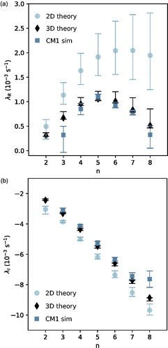
Fig. B1. Scatter plot of the complex eigenfrequencies of the n = 2 MUM in linear systems with (pink) and without (black) acoustic filtering. Different symbol shapes correspond to different combinations of ${ϵ}_{\chi }$ and ${ϵ}_k$ as shown in the legend in the lower left corner of the graph.

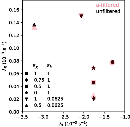
Fig. C1. Scatter plot of the complex eigenfrequencies of the MUMs of the tropical cyclone of Section 4 as determined by the 3D linear model with ${ϵ}_{\chi }={ϵ}_k=1$. The number associated with each data point denotes the value of the azimuthal wavenumber (n) of the MUM. Data is included for computations on G1 (small blue), G2 (medium green) and G4 (large red). Dark (light) symbols indicate modes with ${\text{KE}}_n$ maximised in the lower (middle) troposphere. Note that the G4 data correspond to eigenfrequencies nearest to those of the G2 MUMs, but the associated modes were not verified to dominate time-asymptotic perturbations on G4.

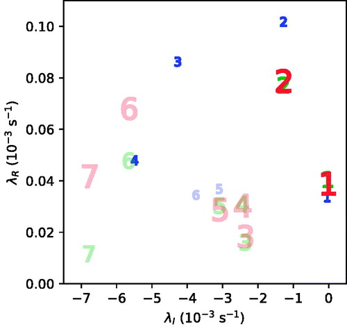
The diamonds in Fig. 17 show the growth rates and oscillation frequencies of the 3D MUMs predicted by the linear model for the tropical cyclone simulated in NS14. The MUMs were first identified as perturbations dominating solutions of the initial value problem with ${ϵ}_{\chi }={ϵ}_k=1$ on a grid $\widetilde{\mathrm{G}2}$ with double the resolution of that used in NS14. The diamonds are centred on values of λ_R and λ_I obtained by recomputing the eigenmodes on a grid $\widetilde{\mathrm{G}4}$ with double the resolution of $\widetilde{\mathrm{G}2}$. Further sensitivity to grid spacing was examined by repeating the computations on the original NS14 grid. Sensitivity to the parameterisations of diabatic forcing and small-scale turbulence were separately examined by reducing ${ϵ}_{\chi }$ to 0 and ${ϵ}_k$ to 0.0625 on $\widetilde{\mathrm{G}2}$ and $\widetilde{\mathrm{G}4}$. The error bar on each diamond covers the full range of values for λ_R or λ_I obtained from all configurations of the linear model; the smallness of the error bars indicates robust results. Note that the plotted eigenfrequencies are confined to n between 2 and 8, which correspond to eigenmodes energetically concentrated near the surface (not shown); a slower growing middle-tropospheric MUM associated with n = 1 is excluded from present consideration.

Figure 17 clearly demonstrates that the eigenfrequencies of the theoretical and simulated 3D MUMs are in good agreement where the latter are inferred from the cleanest monochromatic signals ($4\le n\le 7$). On the other hand, both the growth rates and oscillation frequencies are smaller than those of the MUMs associated with an analogous 2D vortex (circles). The 2D vortex under consideration is modelled after the primary circulation of the NS14 tropical cyclone averaged in z over a layer of thickness d adjacent to the surface. The plotted 2D data points correspond to the means taken from 6 configurations in which $d\in \{1,2,3\}$ km and $K_{2d}\in \{0,{10}^3\}$ m²s^–1. As usual, the error bars extend from the minimum to maximum values of the data set for each n.

In this particular case study, the insensitivity of 3D linear instability theory to the degree of diabatic forcing allowed in the model is consistent with the concentration of modal wave activity inward of the eyewall cloud (NS14). Insensitivity to the reduction of ${ϵ}_k$ seems reasonable given the short e-folding times of the MUMs (15-20 min) relative to the minimum applicable time scale for turbulent diffusion, ${\tau }_k\equiv \min (l_h^2/K_h,l_v^2/K_v)$, in which $l_{h/v}$ is the horizontal/vertical lengthscale relevant to the mode and $K_{h/v}$ is the horizontal/vertical eddy diffusivity. Taking $K_{h/v}\le 200$ m²s^–1 and $l_{h/v}\ge {10}^3$ m yields ${\tau }_k\ge 83$ min.

7. Conclusion

This paper has proposed a method to account for diabatic forcing and inhomogeneous eddy diffusivities in predicting and analysing the dominant instability modes of numerically simulated tropical cyclones. Excluding explicit moisture equations from the linearised model necessitated a partly intuitive parameterisation of the diabatic forcing $S_{\theta }^{\prime }$. The parameterisation considered herein set $S_{\theta }^{\prime }$ proportional to $w\prime$ with the modulating coefficient ${ϵ}_{\chi }{\tilde{\chi }}_b{\partial }_z{\theta }_{\rho b}$ dependent on the local moist thermodynamic conditions of the basic state. A more general parameterisation scheme [Equation (10)(10) $$S{\prime }_{\theta }(r,\phi ,z,t)=\sum _{F,j}\iiint d\tilde{r}d\tilde{\phi }d\tilde{z}\tilde{r}{G}_j^F(\tilde{r},\tilde{\phi },\tilde{z};r,\phi ,z){\widehat{L}}_j^F[F\prime (\tilde{r},\tilde{\phi },\tilde{z},t\left)\right],$$(10) ] was presented for future consideration.

The instability analysis was illustrated for a mature tropical cyclone representative of a category 4 hurricane. The basic state was generated by an axisymmetric numerical simulation with two-moment cloud microphysics and typical settings for the parameterisation of subgrid turbulence. Initial consideration was given to linear systems having vertical and horizontal eddy diffusivities comparable to those regulating the basic state. With the diabatic forcing parameter ${ϵ}_{\chi }$ set to a value between 0 and 1, perturbation growth was commonly dominated by a slowly growing n = 2 eigenmode with deep structure but maximal intensity (${\text{KE}}_n$) in the lower tropospheric region of the inner core. The complex eigenfrequency, spatial structure and energetics of the n = 2 MUM were sensitive to variation of ${ϵ}_{\chi }$. Increasing ${ϵ}_{\chi }$ from 0 to 0.9 gradually stabilised the mode. Further amplification of ${ϵ}_{\chi }$ to 1 introduced a new MUM distinguished in part by having a larger growth rate than any of its predecessors, and by having a slightly positive buoyancy-related contribution to the production of integrated ${\text{KE}}_n$.

Reducing the eddy diffusivities with ${ϵ}_{\chi }$ fixed at either 0.5 or 1 generally changed the nature of the n = 2 instability. For ${ϵ}_{\chi }=0.5$, the original MUM was ultimately replaced by a faster surface-concentrated instability mode whose growth of ${\text{KE}}_n$ involved a much smaller fractional contribution from the term directly linked to the secondary circulation. For ${ϵ}_{\chi }=1$, the original MUM was replaced by a faster instability mode whose growth of ${\text{KE}}_n$ distinctly involved a negative contribution from the buoyancy term and a relatively large positive contribution from the tendency associated with the vertical shear of the primary circulation.

Sensitivity of the foregoing analysis to the parameterisations of diabatic forcing and turbulent transport attests to the importance of details in predicting and understanding tropical cyclone instabilities. Improving the predictive skill of the linear model will require reducing the present degree of uncertainty in the aforementioned parameterisations. Refinements of $S_{\theta }^{\prime }$ and $D{\prime }_{\alpha }$ will come through a combination of theoretical advancements and testing of the linear model against perturbation growth found in state-of-the-art cloud resolving models.

An initial test of our linear model produced encouraging results. The instability analysis showed very good quantitative agreement with the perturbation growth that leads to mesovortex formation slightly inward of the eyewall cloud in a previously conducted CM1 simulation with relatively low diffusivity (NS14). Such agreement helped validate the dynamical core of the linear model. On the other hand, questions regarding the parameterisation schemes were left unresolved. The instability was theoretically too fast for reasonable variants of turbulent transport to have an appreciable effect on its early development. Moreover, the perturbation seemed largely detached from moist processes (NS14). Accordingly, the instability predicted by the linear model showed little sensitivity to switching ${ϵ}_{\chi }$ between 0 and 1.

Acknowledgements

The author thanks Dr. Konstantinos Menelaou and an anonymous reviewer for their comments on this study prior to publication. The author also expresses his gratitude to Dr. George Bryan for providing the cloud resolving model (CM1) used to generate the tropical cyclones whose instabilities were analysed herein. The NS14 study re-examined in Section 6 was made possible through computing allocations from XSEDE and the National Center for Atmospheric Research as noted in the original article.

Disclosure statement

No potential conflict of interest was reported by the author.

Additional information

Funding

Preparation of this paper was partly supported by the National Science Foundation under grant AGS-1743854.

Appendix A. Notes on $S_{\theta }^{\prime }$

The parameterisation of diabatic forcing given by Equation (9(9a) $$\begin{array}{cc}\hfill & S{\prime }_{\theta }={\tilde{\chi }}_b{\partial }_z{\theta }_{\rho b}w\prime \hfill \\ \to \hfill & S_{\theta n}={\tilde{\chi }}_b{\partial }_z{\theta }_{\rho b}{w}_n.\hfill \end{array}$$(9a) b) requires formulas for the partial pressure derivatives of ${\theta }_{\rho }^u$ and ${\theta }_{\rho }^s$ appearing in the definition of χ [Equation (7)(7) $$\chi =H(q_t-q_{v*}){\left(\frac{\partial {\theta }_{\rho }^s}{\partial p}\right)}_{s_m,q_t}+H(q_{v*}-q_t){\left(\frac{\partial {\theta }_{\rho }^u}{\partial p}\right)}_{s_m,q_t},$$(7) ]. SM07 derives the following formulas for the special case of a system with liquid-only condensate: (A1a) $${\left(\frac{\partial {\theta }_{\rho }^u}{\partial p}\right)}_{s_m,q_t}=-\frac{T{R}_d}{c_{pd}p}{\left(\frac{p_a}{p}\right)}^{R_d/c_{pd}}\frac{1+q_t/ϵ}{1+q_t}\left(1-\frac{1+q_t/ϵ}{1+q_t{c}_{pv}/c_{pd}}\right),$$(A1a) (A1b) $$\begin{array}{c}{\left(\frac{\partial {\theta }_{\rho }^s}{\partial p}\right)}_{s_m,q_t}=\hfill \\ -\frac{T{R}_d}{c_{pd}p}{\left(\frac{p_a}{p}\right)}^{R_d/c_{pd}}\frac{1+q_{v*}/ϵ}{1+q_t}\left[1+\frac{c_{pd}{q}_{v*}}{ϵR_d}-\frac{\left(1+\frac{q_{v*}}{ϵ}\right){\left(1+\frac{L_v{q}_{v*}}{R_{d}T}\right)}^2}{1+\frac{q_{v*}{c}_{pv}}{c_{pd}}+\frac{(q_t-q_{v*})c_l}{c_{pd}}+\frac{L_v^2{q}_{v*}(1+q_{v*}/ϵ)}{R_v{c}_{pd}{T}^2}}\right],\hfill \end{array}$$(A1b) in which c_pv is the isobaric specific heat of water vapour, $L_v(T)$ is the latent heat of vapourisation, and c_l is the specific heat of liquid water. For a system with ice-only condensate, the same two equations apply with the following modifications to the saturated air formula: the latent heat of sublimation L_s replaces L_v, and the specific heat of ice c_i replaces c_l. As in the main text, the variable $q_{v*}(p,T)$ represents the vapour mixing ratio at saturation with respect to either liquid or ice, depending on the allowed condensate.

As in reality, the simulated tropical cyclone providing the basic state of Section 4 is complicated by having 3 phases of moisture. To keep the working estimate of $S{\prime }_{\theta }$ relatively simple, the definition of χ that assumes liquid-only (ice-only) condensate is used where $T>T_0$ ($T<T_0$), in which $T_0\equiv 273.15$ K. The temporal averaging of χ that produces χ_b (see Section 4) helps smooth discontinuities at cloud edges and the freezing level. Of further note, the value of q_t substituted into the definition of χ arbitrarily excludes contributions from relatively fast falling hydrometeors such as rain, graupel and snow. The very subtle change to the distribution of ${\tilde{N}}^2$ [Equation (28(28a) $$-\frac{\partial {\theta }_{\rho b}}{\partial z}{w}_n+S_{\theta n}\to -\frac{{\theta }_{\rho b}}{g}{\tilde{N}}^2{w}_n,$$(28a) b)] resulting from such exclusion is minimal compared to the effect of adjusting ${ϵ}_{\chi }$ as in Section 5.1 of the main text.

Section 2.2 indirectly suggested that the condition $\chi \prime {\dot{p}}_b\ll {\chi }_b\dot{p}\prime$ would help justify the assumed proportionality between $S_{\theta }^{\prime }$ and $w\prime \approx -\dot{p}\prime /{\rho }_{b}g$, at least in a system governed by reversible moist-adiabatic thermodynamics. Upon considering the lowest order terms in a multivariable Taylor expansion of $\chi \prime$, one may formulate a stronger version of the preceding inequality for single-wavenumber perturbations as follows: (A2) $$\Gamma \equiv {\left[{\left(\frac{\partial \chi }{\partial p}\right)}_b\frac{\left|p_n\right|{\dot{p}}_b}{{\chi }_b\left|{\dot{p}}_n\right|},{\left(\frac{\partial \chi }{\partial T}\right)}_b\frac{\left|T_n\right|{\dot{p}}_b}{{\chi }_b\left|{\dot{p}}_n\right|},{\left(\frac{\partial \chi }{\partial q_t}\right)}_b\frac{\left|q_{tn}\right|{\dot{p}}_b}{{\chi }_b\left|{\dot{p}}_n\right|}\right]}_{\text{mx}}\ll 1,$$(A2) in which ${[\dots ]}_{\text{mx}}$ denotes the maximum order of magnitude among the bracketed items. Violation of inequality (A2) evaluated with the basic state and perturbation fields of our linear model would cast doubt on the adequacy of having formulated $S_{\theta }^{\prime }$ as a linear function solely of $w\prime$. The forthcoming evaluation will take perturbation amplitudes from the n = 2 MUM of the linear system with ${ϵ}_{\chi }={ϵ}_k=1$, as displayed in Section 5.1. A conservative estimate will be used for the order-of-magnitude of $\left|q_{tn}\right|$ that is not explicitly provided by the linear model.

The following analysis is restricted to the interior region of the eyewall updraft, defined to be where $w_b\ge 2.6$ m s⁻¹. In this saturated region of the tropical cyclone, $\chi ={({\partial }_p{\theta }_{\rho }^s)}_{s_m,q_t}$. The partial derivatives of χ at $(p,T,q_t)=(p_b,T_b,q_{tb})$ are accurately obtained from basic finite differencing without the need to derive lengthy analytical formulas. The pressure variables appearing in (A2) are given by (A3a) $$p_n=\left(\frac{{\theta }_{\rho n}}{{\theta }_{\rho b}}+\frac{{\rho }_n}{{\rho }_b}\right)\frac{c_{pd}}{c_{vd}}{p}_b,$$(A3a) (A3b) $${\dot{p}}_n={\partial }_t{p}_n+u_b{\partial }_r{p}_n+in{\Omega }_b{p}_n+w_b{\partial }_z{p}_n+u_n{\partial }_r{p}_b+w_n{\partial }_z{p}_b,$$(A3b) (A3c) $${\dot{p}}_b=u_b{\partial }_r{p}_b+w_b{\partial }_z{p}_b.$$(A3c) Linearising the relation $T=(1+q_t)\Pi {\theta }_{\rho }/[1+q_{v*}(p,T)/ϵ]$ for air that remains precisely saturated— and using standard formulas (Emanuel, 1994) for the partial derivatives of $q_{v*}$ —yields (A4) $$\begin{array}{c}{T}_n=\frac{T_b}{1+L_b{q}_{v*b}/R_d{T}_b}\left[\left(\frac{R_d}{c_{pd}}+\frac{q_{v*b}}{ϵ}\right)\frac{p_n}{p_b}+\frac{{\theta }_{\rho n}}{{\theta }_{\rho b}}+\frac{q_{tn}}{1+q_{tb}}\right]\hfill \\ \to \left|T_n\right|\sim {\left[\left|{\kappa }_p\frac{p_n}{p_b}+{\kappa }_{\theta }\frac{{\theta }_{\rho n}}{{\theta }_{\rho b}}\right|,\frac{{\kappa }_{\theta }\left|q_{tn}\right|}{1+q_{tb}}\right]}_{\text{mx}},\hfill \end{array}$$(A4) in which ${\kappa }_{\theta }\equiv T_b/(1+L_b{q}_{v*b}/R_d{T}_b)$, ${\kappa }_p\equiv {\kappa }_{\theta }[(R_d/c_{pd})+(q_{v*b}/ϵ)]$, $q_{v*b}=q_{v*}(p_b,T_b)$ and L_b is either $L_v(T_b)$ or L_s if T_b is greater or less than T₀. For simplicity, let us suppose that (A5) $$\left|q_{tn}\right|\sim {ϵ}_q{q}_{tb},$$(A5) in which ${ϵ}_q$ is tentatively set to 0.5, so as to equal 10 times the maximum of $\left|v_n\right|/v_{bm}$.

Two estimates of Γ have been calculated. ${\Gamma }_1$ (${\Gamma }_2$) is obtained by evaluating all 5 variables in each bracketed item of (A2) with their maximum (average) absolute values in the interior region of the eyewall. The marginally reassuring results are ${\Gamma }_1=0.3$ and ${\Gamma }_2=0.2$; smaller values are obtained as ${ϵ}_q\to 0$.

Appendix B. Acoustic filtering

It is common practice to use an anelastic approximation of the equations of motion when acoustic waves are deemed unimportant to the instabilities of interest (NM02; Hodyss and Nolan, 2008). The effect of acoustic filtering is considered herein by implementing the following approximation of Equation (3(3a) $$\begin{array}{l}\frac{\partial u_n}{\partial t}=-\frac{\partial u_b{u}_n}{\partial r}-in{\Omega }_b{u}_n-w_b\frac{\partial u_n}{\partial z}+{\xi }_b{v}_n-\frac{\partial u_b}{\partial z}{w}_n\\ -c_{pd}\frac{\partial {\Pi }_b}{\partial r}{\theta }_{\rho n}-\mu {\theta }_{\rho b}\frac{\partial }{\partial r}\left[\frac{{\Pi }_b}{{\theta }_{\rho b}}{\theta }_{\rho n}+\frac{{\Pi }_b}{{\rho }_b}{\rho }_n\right]+{\tilde{D}}_{un}\end{array}$$(3a) e): (B1) $$\frac{in{\rho }_b{v}_n}{r}=-\frac{1}{r}\frac{\partial r{\rho }_b{u}_n}{\partial r}-\frac{\partial {\rho }_b{w}_n}{\partial z}.$$(B1) Details of the implementation are provided below.

Recall from Section 3 that the unfiltered linearised equations of motion can be written $d{\mathbf{x}}_n/dt={\mathbf{M}}_n{\mathbf{x}}_n$, in which x_n is a vector representation of all prognostic perturbation fields at all grid points. Let ${\mathbf{y}}_n^F$ denote the subvector of x_n representing field F_n. The acoustically filtered system consists of three prognostic equations of the form (B2a) $$\frac{d{\mathbf{y}}_n^F}{dt}=\sum _{\tilde{F}\in \{u,v,w,{\theta }_{\rho },\rho \}}{\mathbf{M}}_n^{F\tilde{F}}{\mathbf{y}}_n^{\tilde{F}},$$(B2a) in which $F\in \{u,w,{\theta }_{\rho }\}$ and ${\mathbf{M}}_n^{F\tilde{F}}$ is the submatrix of M_n accounting for the tendency of ${\mathbf{y}}_n^F$ directly dependent on ${\mathbf{y}}_n^{\tilde{F}}$. The equations for the perturbations of azimuthal velocity and density are diagnostic. The azimuthal velocity equation is given by (B2b) $${\mathbf{y}}_n^v=\sum _{\tilde{F}\in \{u,w\}}{\mathbf{V}}_n^{\tilde{F}}{\mathbf{y}}_n^{\tilde{F}},$$(B2b) in which ${\mathbf{V}}_n^u$ and ${\mathbf{V}}_n^w$ are the coefficient matrices relating ${\mathbf{y}}_n^v$ to ${\mathbf{y}}_n^u$ and ${\mathbf{y}}_n^w$ according to the discretization of Equation (B1)(B1) $$\frac{in{\rho }_b{v}_n}{r}=-\frac{1}{r}\frac{\partial r{\rho }_b{u}_n}{\partial r}-\frac{\partial {\rho }_b{w}_n}{\partial z}.$$(B1) . The density equation is given by (B2c) $$\begin{array}{c}[{\mathbf{M}}_n^{v\rho }-\sum _{F\in \{u,w\}}{\mathbf{V}}_n^F{\mathbf{M}}_n^{F\rho }]{\mathbf{y}}_n^{\rho }=-\sum _{F\in \{u,w,{\theta }_{\rho }\}}{\mathbf{M}}_n^{vF}{\mathbf{y}}_n^F-\sum _{F\in \{u,w\}}{\mathbf{M}}_n^{vv}{\mathbf{V}}_n^F{\mathbf{y}}_n^F\hfill \\ +\sum _{F\in \{u,w\}\tilde{F}\in \{u,w,{\theta }_{\rho }\}}{\mathbf{V}}_n^F{\mathbf{M}}_n^{F\tilde{F}}{\mathbf{y}}_n^{\tilde{F}}+\sum _{F\in \{u,w\}\tilde{F}\in \{u,w\}}{\mathbf{V}}_n^F{\mathbf{M}}_n^{Fv}{\mathbf{V}}_n^{\tilde{F}}{\mathbf{y}}_n^{\tilde{F}}.\hfill \end{array}$$(B2c) The preceding formula for ${\mathbf{y}}_n^{\rho }$ is obtained by substituting (B2b) and (B2a) for $F\in \{u,w\}$ into the prognostic azimuthal velocity equation of the unfiltered system. Note that the foregoing acoustically filtered model applies only for $n\ge 1$, owing to a derivation from equations where v_n and ρ_n are multiplicatively coupled to n. An alternative formulation valid for $n\ge 0$ would seem possible by (say) switching the roles of w_n and v_n as prognostic and diagnostic variables.

As suggested earlier, acoustic filtering is expected to have minimal consequence on the primary inner core instability of a tropical cyclone. Consider the tropical cyclone of Section 4. The unfiltered n = 2 MUM is described in Section 5 for various combinations of ${ϵ}_{\chi }$ and ${ϵ}_k$ in the linear model. The acoustically filtered MUM is here found (on G2) by initialising Equations (B2(B2a) $$\frac{d{\mathbf{y}}_n^F}{dt}=\sum _{\tilde{F}\in \{u,v,w,{\theta }_{\rho },\rho \}}{\mathbf{M}}_n^{F\tilde{F}}{\mathbf{y}}_n^{\tilde{F}},$$(B2a) a)–(B2c) with ${\mathbf{y}}_n^u,{\mathbf{y}}_n^w$ and ${\mathbf{y}}_n^{{\theta }_{\rho }}$ of the unfiltered MUM and integrating forward in time over several e-folding periods. Under ordinary circumstances, the perturbation is quickly dominated by the filtered MUM. Figure B1 verifies that the complex eigenfrequencies of the filtered and unfiltered instability modes hardly differ, regardless of the selected parameters regulating the strengths of diabatic forcing and turbulent transport.

Appendix C. Sensitivity of MUMs to the computational grid

In Section 5, a MUM was provisionally equated to the eigenmode that dominates a perturbation within 1 day of initialising the linear model [Equation (20)(20) $$\frac{d{\mathbf{x}}_n}{dt}={\mathbf{M}}_n{\mathbf{x}}_n,$$(20) ] with random noise on a grid (G2) having double the resolution— in both r and z —of the CM1 grid used to generate the basic state (G1). The MUMs of G1 are readily found by a similar procedure. Figure C1 displays the complex eigenfrequencies associated with the MUMs of both G1 (blue) and G2 (green) for $0<n<8$ when the linear model is parameterized with ${ϵ}_{\chi }={ϵ}_k=1$. Note that no discernible instabilities could be seen for n = 0 or n = 8. Also shown are solutions to the eigenproblem on a grid (G4, red) with quadruple the resolution of G1. Each G4 data point is obtained from an algorithm that seeks a solution for the complex eigenfrequency (λ) closest to that of the G2 MUM.

The system under present consideration exhibits a somewhat complicated sensitivity to grid spacing. The n = 1 mode is virtually invariant with increasing resolution. The oscillation frequency (λ_I) of the n = 2 mode is also robust, but the growth rate on G1 exceeds that on G4 by 29%. The values of λ_R (for n = 2) on G2 and G4 are deemed closer to the continuum limit based on their modest 2% difference. All of the modes on G1 that are shown for $1\le n\le 4$ have maximal ${\text{KE}}_n$ near the surface. Whereas the properties of the modes with n = 1 and n = 2 are fairly insensitive to increasing resolution, the n = 3 and 4 modes on G1 are fragile and superceded by middle tropospheric instabilities on G2 and G4. All of the dominant instabilities at higher wavenumbers have maximal ${\text{KE}}_n$ in the middle troposphere. It is notable that increasing the resolution for cases in which n exceeds 5 markedly accelerates the instabilities. Moreover, the resolution required to establish less than 10% uncertainty in λ_R at high-n appears to be greater than that of G4.

Appendix D. The 2D eigenproblem

The equations of motion governing a nondivergent 2D vortex with kinematic viscosity $K_{2d}$ are given below: (D1a) $${\partial }_t\zeta +\mathbf{u}·{\nabla }_h\zeta =K_{2d}{\nabla }_h^2\zeta ,$$(D1a) (D1b) $$\mathbf{u}=\widehat{z}\times {\nabla }_h\psi ,$$(D1b) (D1c) $${\nabla }_h^2\psi =\zeta ,$$(D1c) in which ζ is the vertical vorticity (the subscript z is unnecessary and dropped in this appendix) associated with the horizontal velocity field $\mathbf{u}$, ψ is the streamfunction, and ${\nabla }_h$ is the horizontal gradient operator. Nonzero viscosity will cause the gradual diffusion of an arbitrary axisymmetric state that is characterised by the vorticity distribution ${\zeta }_b(r)$. A linearised model for asymmetric perturbation growth is justifiable if axisymmetric diffusion occurs much more slowly than the instability. Extension of the linearised model to values of $K_{2d}$ where axisymmetric diffusion and asymmetric perturbation growth have commensurate time scales is technically improper, but is deemed reasonable for the purpose of illustrating modal sensitivity to the magnitude of viscosity.

The asymmetric ($n\ge 1$) eigenmodes of an axisymmetric vortex are perturbations of the form $\zeta \prime =Z(r)e^{in\phi +\lambda t}+c.c.$, in which $c.c.$ denotes the complex conjugate of the preceding term. Substituting the eigenmode solution into the linearised equations of motion derived from Equations (D1(D1a) $${\partial }_t\zeta +\mathbf{u}·{\nabla }_h\zeta =K_{2d}{\nabla }_h^2\zeta ,$$(D1a) a)–(D1c) yields (D2a) $$(i\lambda -n{\Omega }_b)Z+\frac{n}{r}\frac{d{\zeta }_b}{dr}\Psi -i{K}_{2d}{\nabla }_n^{2}Z=0,$$(D2a) in which ${\Omega }_b(r)$ is the angular velocity corresponding to ζ_b, ${\nabla }_n^2\Psi =Z,{\nabla }_n^2\equiv {\partial }_{rr}+r^{-1}{\partial }_r-n^2/r^2$, and ${\partial }_{rr}\equiv {\partial }_r{\partial }_r$. A formal solution for the wavefunction of $\psi \prime$ consistent with regularity at the origin and $u\prime =0$ at r = r_B is (D2b) $$\Psi \left(r\right)=-\frac{1}{2n}{\int }_0^{r_B}d\tilde{r}\tilde{r}{\left(\frac{r_{<}}{r_{>}}\right)}^n\left[1-{\left(\frac{r_{>}}{r_B}\right)}^{2n}\right]Z\left(\tilde{r}\right),$$(D2b) in which $r_{<}$ ($r_{>}$) is the lesser (greater) of $\tilde{r}$ and r (Schecter et al., 2000). The second outer boundary condition ${\partial }_r(v\prime /r)=0$ combined with $u\prime =0$ amounts to $Z=2r^{-1}d\Psi /dr$ at r = r_B. Substituting (D2b) into both (D2a) and the preceding outer boundary condition eliminates $\Psi$ from the eigenproblem. Subsequent discretization of the radial coordinate yields a standard matrix eigenproblem of the form $\mathbf{M}\mathbf{x}=\lambda \mathbf{x}$, in which $\mathbf{x}$ is a vector containing the values of Z on each grid point. The 2D results of Section 5.3 and 6 correspond to solutions of the preceding eigenproblem; the outer boundary condition on $v\prime$ is obviated for computations in which $K_{2d}=0$. Selected results were successfully cross-checked against independent solutions of the 3D model set up with a thin barotropic vortex sandwiched in between rigid free-slip walls at z = 0 and 0.5 km.

Appendix E. The Helmholtz decomposition

The Fourier transform of the horizontal velocity perturbation associated with a 3D instability mode can be decomposed into the following sum of irrotational (superscript-$\varphi$) and nondivergent (superscript-ψ) components: (E1a) $$\left[\begin{array}{c}{u}_n\\ v_n\end{array}\right]=\left[\begin{array}{c}{u}_n^{\varphi }+u_n^{\psi }\\ v_n^{\varphi }+v_n^{\psi }\end{array}\right]$$(E1a) in which (E1b) $$\left[\begin{array}{c}{u}_n^{\varphi }\\ v_n^{\varphi }\end{array}\right]=\left[\begin{array}{c}{\partial }_r{\varphi }_n\\ in{\varphi }_n/r\end{array}\right],\left[\begin{array}{c}{u}_n^{\psi }\\ v_n^{\psi }\end{array}\right]=\left[\begin{array}{c}-in{\psi }_n/r\\ {\partial }_r{\psi }_n\end{array}\right],$$(E1b) and (E1c) $${\nabla }_n^2\left[\begin{array}{c}{\varphi }_n\\ {\psi }_n\end{array}\right]=\left[\begin{array}{c}{\sigma }_n\\ {\zeta }_{zn}\end{array}\right].$$(E1c)

The boundary conditions at the origin are regularity of the velocity potential ${\varphi }_n$ and streamfunction ψ_n; the implemented boundary conditions at r_B consistent with u_n = 0 are ${\partial }_r{\varphi }_n=0$ and ${\psi }_n=0$. The velocity fields depicted in Figs. 16d,f correspond to $\mathbf{u}\prime {}^{\varphi }=\mathbf{u}\prime -\mathbf{u}\prime {}^{\psi }$, in which $\mathbf{u}\prime =(u_n,v_n)e^{in\phi }+c.c.$ and $\mathbf{u}\prime {}^{\varphi /\psi }=(u_n^{\varphi /\psi },v_n^{\varphi /\psi })e^{in\phi }+c.c.$

References

- Antkowiak, A. and Brancher, P. 2004. Transient energy growth for the Lamb-Oseen vortex. Phys. Fluids 16, L1–L4. doi:10.1063/1.1626123
- Bryan, G. 2008. On the computation of pseudoadiabatic entropy and equivalent potential temperature. Mon. Wea. Rev. 136, 5239–5245. doi:10.1175/2008MWR2593.1
- Bryan, G. H. and Fritsch, J. M. 2002. A benchmark simulation for moist nonhydrostatic numerical models. Mon. Wea. Rev. 130, 2917–2928. doi:10.1175/1520-0493(2002)130<2917:ABSFMN>2.0.CO;2
- Bryan, G. H. and Rotunno, R. 2009. The maximum intensity of tropical cyclones in axisymmetric numerical model simulations. Mon. Wea. Rev. 137, 1770–1789. doi:10.1175/2008MWR2709.1
- Donelan, M. A., Haus, B. K., Reul, N., Plant, W. J., Stiassnie, M. and co-authors. 2004. On the limiting aerodynamic roughness of the ocean in very strong winds. Geophys. Res. Lett. 31, L18306. 1–5.
- Drennan, W. M., Zhang, J. A., French, J. R., McCormick, C. and Black, P. G. 2007. Turbulent fluxes in the hurricane boundary layer. Part II: Latent heat flux. J. Atmos. Sci. 64, 1103–1115. doi:10.1175/JAS3889.1
- Dunion, J. P. 2011. Rewriting the climatology of the tropical North Atlantic and Caribbean Sea atmosphere. J. Climate 24, 893–908. doi:10.1175/2010JCLI3496.1
- Durran, D. R. and Klemp, J. B. 1982. On the effects of moisture on the Brunt-Väisälä frequency. J. Atmos. Sci. 39, 2152–2158. doi:10.1175/1520-0469(1982)039<2152:OTEOMO>2.0.CO;2
- Eliassen, A. 1951. Slow thermally or frictionally controlled meridional circulation in a circular vortex. Astrophysica Norvegica 5, 19–60.
- Emanuel, K. A. 1986. An air sea interaction theory for tropical cyclones. Part I: Steady state maintenance. J. Atmos. Sci. 43, 585–604. doi:10.1175/1520-0469(1986)043<0585:AASITF>2.0.CO;2
- Emanuel, K. A. 1994. Atmospheric Convection. Oxford University Press, New York, p. 580.
- Fairall, C. W., Bradley, E. F., Hare, J. E., Grachev, A. A. and Edson, J. B. 2003. Bulk parameterization of air-sea fluxes: Updates and verification for the COARE algorithm. J. Climate 16, 571–591. doi:10.1175/1520-0442(2003)016<0571:BPOASF>2.0.CO;2
- Gall, R. L. 1983. A linear analysis of the multiple vortex phenomenon in simulated tornadoes. J. Atmos. Sci. 40, 2010–2024. doi:10.1175/1520-0469(1983)040<2010:ALAOTM>2.0.CO;2
- Hakim, G. J. 2011. The mean state of axisymmetric hurricanes in statistical equilibrium. J. Atmos. Sci. 68, 1364–1376. doi:10.1175/2010JAS3644.1
- Hendricks, E. A. and Schubert, W. H. 2010. Adiabatic rearrangement of hollow PV towers. J. Adv. Model. Earth Syst. 2, 1–19.
- Hendricks, E. A., Schubert, W. H., Chen, Y-h., Kuo, H.-C. and Peng, M. S. 2014. Hurricane eyewall evolution in a forced shallow water model. J. Atmos. Sci. 71, 1623–1643. doi:10.1175/JAS-D-13-0303.1
- Hodyss, D. and Nolan, D. S. 2008. The Rossby-inertia-buoyancy instability in baroclinic vortices. Phys. Fluids 20, 096602. 1–21.
- Kossin, J. P. and Schubert, W. H. 2001. Mesovortices, polygonal flow patterns, and rapid pressure falls in hurricane-like vortices. J. Atmos. Sci. 58, 2196–2209. doi:10.1175/1520-0469(2001)058<2196:MPFPAR>2.0.CO;2
- Kwon, Y. C. and Frank, W. M. 2005. Dynamic instabilities of simulated hurricane-like vortices and their impacts on the core structure of hurricanes. Part I: Dry experiments. J. Atmos. Sci. 62, 3955–3973. doi:10.1175/JAS3575.1
- Lahaye, N. and Zeitlin, V. 2016. Understanding instabilities of tropical cyclones and their evolution with a moist convective rotating shallow-water model. J. Atmos. Sci. 73, 505–523. doi:10.1175/JAS-D-15-0115.1
- Menelaou, K., Schecter, D. A. and Yau, M. K. 2016. On the relative contribution of inertia-gravity wave radiation to asymmetric instabilities in tropical cyclone-like vortices. J. Atmos. Sci. 73, 3345–3370. doi:10.1175/JAS-D-15-0360.1
- Montgomery, M. T. and Shapiro, L. J. 1995. Generalized Charney-Stern and Fjortoft theorems for rapidly rotating vortices. J. Atmos. Sci. 52, 1829–1833. doi:10.1175/1520-0469(1995)052<1829:GCAFTF>2.0.CO;2
- Morrison, H., Curry, J. A. and Khvorostyanov, V. I. 2005. A new double-moment microphysics parameterization for application in cloud and climate models. Part I: Description. J. Atmos. Sci. 62, 1665–1677. doi:10.1175/JAS3446.1
- Morrison, H., Thompson, G. and Tatarskii, V. 2009. Impact of cloud microphysics on the development of trailing stratiform precipitation in a simulated squall line: Comparison of one-and two-moment schemes. Mon. Wea. Rev. 137, 991–1007. doi:10.1175/2008MWR2556.1
- Naylor, J. and Schecter, D. A. 2014. Evaluation of the impact of moist convection on the development of asymmetric inner core instabilities in simulated tropical cyclones. J. Adv. Model. Earth Syst. 6, 1027–1048. doi:10.1002/2014MS000366
- Nolan, D. S. 2013. Three-dimensional instabilities in tornado-like vortices with secondary circulations. J. Fluid Mech. 711, 61–100.
- Nolan, D. S. and Farrell, B. F. 1999. Generalized stability analysis of asymmetric disturbances in one- and two-celled vortices maintained by radial inflow. J. Atmos. Sci. 56, 1282–1307. doi:10.1175/1520-0469(1999)056<1282:GSAOAD>2.0.CO;2
- Nolan, D. S. and Montgomery, M. T. 2002. Nonhydrostatic, three-dimensional perturbations to balanced, hurricane-like vortices. Part I: linearized formulation, stability, and evolution. J. Atmos. Sci. 59, 2989–3020. doi:10.1175/1520-0469(2002)059<2989:NTDPTB>2.0.CO;2
- Rogers, R., Aberson, S., Aksoy, A., Annane, B., Black, M. and coauthors. 2013. NOAA’s hurricane intensity forecasting experiment: A progress report. Bull. Am. Meteor. Soc. 94, 859–882. doi:10.1175/BAMS-D-12-00089.1
- Rotunno, R. 1978. A note on the stability of a cylindrical vortex sheet. J. Fluid Mech. 87, 761–771. doi:10.1017/S0022112078001871
- Rozoff, C. M., Kossin, J. P., Schubert, W. H. and Mulero, P. J. 2009. Internal control of hurricane intensity variability: The dual nature of potential vorticity mixing. J. Atmos. Sci. 66, 133–147. doi:10.1175/2008JAS2717.1
- Schecter, D. A., Dubin, D. H. E., Cass, A. C., Driscoll, C. F., Lansky, I. M. and co-authors. 2000. Inviscid damping of asymmetries on a two-dimensional vortex. Phys. Fluids 12, 2397–2412. doi:10.1063/1.1289505
- Schecter, D. A. and Menelaou, K. 2017. Note on analyzing perturbation growth in a tropical cyclone-like vortex radiating inertia-gravity waves. J. Atmos. Sci. 74, 1561–1571. doi:10.1175/JAS-D-16-0289.1
- Schecter, D. A. and Montgomery, M. T. 2003. On the symmetrization rate of an intense geophysical vortex. Dyn. Atmos. Oceans 37, 55–88. doi:10.1016/S0377-0265(03)00015-0
- Schecter, D. A. and Montgomery, M. T. 2004. Damping and pumping of a vortex Rossby wave in a monotonic cyclone: critical layer stirring versus inertia-buoyancy wave emission. Phys. Fluids 16, 1334–1348. doi:10.1063/1.1651485
- Schecter, D. A. and Montgomery, M. T. 2007. Waves in a cloudy vortex. J. Atmos. Sci. 64, 314–337. doi:10.1175/JAS3849.1
- Schubert, W. H., Montgomery, M. T., Taft, R. K., Guinn, T. A., Fulton, S. R. and co-authors. 1999. Polygonal eyewalls, asymmetric eye contraction, and potential vorticity mixing in hurricanes. J. Atmos. Sci. 56, 1197–1223. doi:10.1175/1520-0469(1999)056<1197:PEAECA>2.0.CO;2
- Shapiro, L. J. and Montgomery, M. T. 1993. A three-dimensional balance theory for rapidly rotating vortices. J. Atmos. Sci. 50, 3322–3335. doi:10.1175/1520-0469(1993)050<3322:ATDBTF>2.0.CO;2
- Smith, R. A. and Rosenbluth, M. N. 1990. Algebraic instability of hollow electron columns and cylindrical vortices. Phys. Rev. Lett. 64, 649–652. doi:10.1103/PhysRevLett.64.649
- Walko, R. and Gall, R. 1984. A two-dimensional linear stability analysis of the multiple vortex phenomenon. J. Atmos. Sci. 41, 3456–3471. doi:10.1175/1520-0469(1984)041<3456:ATDLSA>2.0.CO;2
- Zhang, J. A. and Montgomery, M. T. 2012. Observational estimates of the horizontal eddy diffusivity and mixing length in the low-level region of intense hurricanes. J. Atmos. Sci. 69, 1306–1316. doi:10.1175/JAS-D-11-0180.1
- Zhang, J. A., Rogers, R. F., Nolan, D. S. and Marks, F. D. Jr, 2011. On the characteristic height scales of the hurricane boundary layer. Mon. Wea. Rev. 139, 2523–2535. doi:10.1175/MWR-D-10-05017.1
Appendix A. Notes on