Large-scale secondary circulations in a limited area model – the impact of lateral boundaries and resolution

Abstract

Within their domain, regional climate and weather forecasting models deviate from the driving data. Small-scale deviations are a desired effect of adding regional details. There are, however, also deviations of the large-scale circulation, which can be caused by orographic effects and depend on the large-scale flow condition. These ‘secondary circulations’ (SCs) are confined to the model domain due to the prescribed boundary conditions. Here, the impact of different regional model configurations on the SC is analysed in a case study for the European region using an ensemble approach. It is shown that at 500 hPa, vortices of the SC have diameters on the order of several thousand kilometres and are related to wind speed anomalies of more than 5 m/s and geopotential height anomalies of more than 5 dam. The spatial structure and the amplitude of the SC strongly depend on the location of the lateral boundaries. The impact of the boundary location on the anomalies is on the same order of magnitude as the anomalies themselves. The resolution of the regional model, as well as the application of spectral nudging and a smoothed topography, affects mainly the amplitude of the SC, but not the spatial structure.

Keywords:

• Limited area model
• regional climate model
• COSMO-CLM
• secondary circulation
• boundary effects
• orographic effects

1. Introduction

Regional climate models (RCMs) or, more general, limited area models are used to downscale atmospheric states to resolutions on the order of 1 to 50 km. This process involves the interpolation of the output data of the coarser resolved driving model to the RCM grid, which is then used as the initial state at the start of a simulation on the whole domain and prescribed at the lateral boundaries while integrating the model equations. This method is referred to as the one-way nesting technique. As a simulation is run, an RCM develops the atmospheric states on its finer grid, for example due to the influence of better resolved orography or due to other finer scale processes not represented in the coarser driving data. To damp spurious reflections of smaller scale waves at the lateral boundaries, a relaxation of the boundary conditions is applied, which ensures a smooth transition between the driving data and the interior of the RCM domain within a buffer zone of several grid boxes at the boundaries (Davies, 1976). However, RCMs do not only add variability on smaller scales, but they also deviate from the driving data on larger scales, which are also resolved in the data prescribed at the boundaries (e.g. Miguez-Macho et al., 2004; Becker et al., 2015).

It is discussed whether large-scale deviations of RCMs from the driving data are desired or not (von Storch et al., 2000). While RCMs generally perform better for the medium spatial scales, this is not always the case for the larger spatial scales (Feser et al., 2011). However, it was shown that RCMs are also able to improve the large scales of the driving data, if the model domain is sufficiently large (Diaconescu and Laprise, 2013). On the other hand, large-scale deviations between RCM and driving data can lead to artificial gradients and instabilities at the lateral boundaries of the RCM. For example, Jones et al. (1995) find significant distortions at the grid points adjacent to the buffer zone. A common suggestion is thus to exclude grid boxes near the lateral boundaries when analysing RCM data. As another effect, RCMs can develop an internal circulation which considerably differs from that of the driving model (Becker et al., 2015).

To prevent an RCM from deviating too much from the driving data on larger scales in the inner model domain, a spectral nudging approach has been suggested by von Storch et al. (2000). Here, the driving data additionally influence the large-scale part of the spatial spectrum within the whole model domain, while the small-scale part can freely develop. In idealised experiments, the spectral nudging approach can reduce biases in RCM simulations by removing imbalances caused by large‐scale features in the centre of the domain, which disagree with the solution imposed at the boundaries (Radu et al., 2008). However, spectral nudging assumes that the large scales in the driving data are correct and that there is no strong feedback from the small to the large scales.

While the relaxation of the lateral boundary conditions helps to damp spurious reflections of smaller scale waves at the lateral boundaries, there is no mechanism to handle interactions between larger scale waves with the boundary. For example, Miguez-Macho et al. (2004) find large-scale anomalies in the upper-tropospheric wind fields in RCM simulations covering North America. They assume that these anomalies are caused by synoptic-scale waves, which are initiated by the Rocky Mountains within the RCM domain and which are subsequently reflected at the lateral boundaries. This is consistent with other studies showing that mountains affect the large-scale atmospheric circulation, for example by modulating the phase and amplitude of planetary waves (Broccoli and Manabe, 1992) or by blocking the large-scale flow (Kljun et al., 2001)

Becker et al. (2015) find similar anomalies as Miguez-Macho et al. (2004) in an RCM simulation covering the European region. Here, the Alps are responsible for modifications of the large-scale flow. These large-scale modifications relative to the driving data, caused by the better resolved topography, cannot exit the lateral boundaries due to the prescribed boundary conditions. That leads to the development of large-scale secondary circulations (SCs) in the RCM wind fields relative to the driving data. Vortices in the SC fields are referred to as ‘secondary vortices’. Becker et al. (2015) suppose that the SC directly links the ‘desired’ effects caused by a higher resolved topography within the domain with ‘non-desired’, artificial effects caused by the lateral boundaries. While they show that the SC depends strongly on the direction and strength of the large-scale flow conditions in the Alpine region, it remains an open question how the SC is affected by the specific location of the lateral boundaries.

In general, the specific location and the size of the RCM domain are properties that can strongly influence the result of an RCM simulation, which has been shown in several studies (e.g. Jones et al., 1995; Bhaskaran et al., 1996; Goswami et al., 2012; Larsen et al., 2013). For example, the large-scale anomalies in the upper-tropospheric wind fields found by Miguez-Macho et al. (2004) change their amplitude and shape if the domain is shifted, which could be a direct effect of the SC.

The aim of this work is to study the impact of the model domain configuration on the SC. This is done by simulating a specific atmospheric flow condition with a north-westerly flow crossing the Alps, which induces an intense SC in the RCM, as shown in Becker et al. (2015). In most studies, which analyse the impact of domain size on RCM simulations, all model boundaries are moved simultaneously. Here, the effect of moving individual boundaries is analysed. Furthermore, the impact of the RCM resolution and the application of spectral nudging and a smoothed topography on the SC is analysed.

This article is organised as follows: in Section 2, the experimental set-up and the computation of the ensemble statistics are described. The results of the simulations are analysed in Section 3 concerning the impact of the experimental set-up of the RCM on the characteristics of the SC. Section 4 contains a discussion and in Section 5 final conclusions and recommendations are presented.

2. Models and experimental set-up

The RCM COSMO-CLM (CCLM; Rockel et al., 2008; Doms et al., 2011) version 4.8 is used to perform a series of ensemble simulations with different locations of the lateral boundaries, resolutions and other configurations. The CCLM is a non-hydrostatic model, based on the Local Model (LM) of the German Weather Service, developed by the Consortium of Small-scale Modelling (COSMO) and the Climate Limited-area Modelling-Community (CLM-Community).

The set-up of the CCLM domain used in this work as a reference set-up is equal to the one described in Hollweg et al. (2008) and has been used in several other studies afterwards (e.g. Kunz et al., 2010; Costa et al., 2012; Reyer et al., 2014, Becker et al. 2015). The domain size is similar to the EURO-CORDEX domain. The horizontal resolution is 0.165° in a rotated spherical coordinate system, corresponding to a grid spacing of about 18 km. A height-based terrain-following hybrid vertical coordinate system with 32 layers is used, with the highest vertical layer at approximately 21 km height. Above a height of approximately 11 km, a damping layer is applied, where the RCM variables are partly relaxed to the driving data to prevent the reflection of gravity waves at the model top.

As in Hollweg et al. (2008), a simulation with the coupled atmosphere–ocean global climate model fifth-generation European Centre/Hamburg (ECHAM)/Max-Planck Institute ocean model (Jungclaus et al., 2006) is used to provide the initial and lateral boundary conditions for the CCLM simulations. The ECHAM simulation was carried out for the Fourth Assessment Report of the Intergovernmental Panel on Climate Change (Roeckner et al., 2006) and has a horizontal resolution of T63 (1.875°). It was initialised from a pre-industrial control run and forced with observed CO₂ concentrations for the time period 1860–2000. The 6-hourly ECHAM output is used to force the CCLM using the one-way nesting approach.

To study the effect of different model configurations on the SC, it is necessary to select an appropriate time period for the simulations. An ensemble of long-term climate simulations with a large set of different model configurations is computationally infeasible. Therefore, we selected a time period with a persistent large-scale flow creating a strong and robust pattern in the SC. The longest period with similar flow conditions and a strong SC (as identified by Becker et al., 2015 in the ECHAM model run) consists of a period with a length of 108 h. Subsequently, we focus on this single period, referred to as the ‘analysis period’.

The analysis period is simulated with the CCLM using different model configurations, which are summarised in Table 1. The reference simulation (REF) has the grid configuration as used in Hollweg et al. (2008) and Becker et al. (2015), with a horizontal resolution of 0.165° and 257 × 271 grid boxes. REF covers Europe as well as parts of the North Atlantic and North Africa. Based on REF, a series of simulations are performed with incremental shifts of the northern, eastern, southern and western model boundary. Furthermore, additional simulations are computed with a very large domain, with different horizontal resolutions, with the use of spectral nudging and with a smoothed topography of the CCLM.

Table 1. Model configurations used for CCLM simulations. The shifts of the model boundaries are given as number of grid boxes, with positive values indicating a shift away from the centre of the domain.

Name	Horizontal resolution	Shift of lateral boundaries				Domain size	Filtered orography	Spectral nudging
		North	East	South	West
REF	0.165°	0	0	0	0	257 × 271	no	no
N − 64	0.165°	−64	0	0	0	257 × 207	no	no
N − 32	0.165°	−32	0	0	0	257 × 239	no	no
N + 32	0.165°	+32	0	0	0	257 × 303	no	no
N + 64	0.165°	+64	0	0	0	257 × 335	no	no
E − 64	0.165°	0	−64	0	0	193 × 271	no	no
E − 32	0.165°	0	−32	0	0	225 × 271	no	no
E + 32	0.165°	0	+32	0	0	289 × 271	no	no
E + 64	0.165°	0	+64	0	0	321 × 271	no	no
S − 64	0.165°	0	0	−64	0	257 × 207	no	no
S − 32	0.165°	0	0	−32	0	257 × 239	no	no
S + 32	0.165°	0	0	+32	0	257 × 303	no	no
S + 64	0.165°	0	0	+64	0	257 × 335	no	no
W − 64	0.165°	0	0	0	−64	193 × 271	no	no
W − 32	0.165°	0	0	0	−32	225 × 271	no	no
W + 32	0.165°	0	0	0	+32	289 × 271	no	no
W + 64	0.165°	0	0	0	+64	321 × 271	no	no
LARGE	0.165°	+125	+125	+125	+125	507 × 521	no	no
RES33	0.330°	0	0	0	0	129 × 136	no	no
RES66	0.660°	0	0	0	0	65 × 68	no	no
SN	0.165°	0	0	0	0	257 × 271	no	yes
FILT	0.165°	0	0	0	0	257 × 271	yes	no

For each configuration listed in Table 1, an ensemble of five CCLM simulations is computed. Each of the five ensemble members covers the 108 h of the selected analysis period, but each member has a different spin-up time of 10, 15, 20, 25 and 30 days prior to the first time step of the analysis period. For the following analysis, the ensemble mean and ensemble standard deviation are calculated for different model variables using the temporal average of all 6-hourly time steps within the analysis period.

The ensemble mean wind vector differences between CCLM and ECHAM, which we call the SC, are as follows: (1) $${\Delta \overrightarrow{v}}_{\mathit{\text{mean}}}=\left(\genfrac{}{}{0pt}{}{\frac{1}{N}{\sum }_{i=1}^N{u}_{\mathit{\text{CCLM}},i}-u_{\mathit{\text{ECHAM}}}}{\frac{1}{N}{\sum }_{i=1}^N{v}_{\mathit{\text{CCLM}},i}-v_{\mathit{\text{ECHAM}}}}\right),$$(1) where $N$ is the total number of ensemble members, $u_{\mathit{\text{CCLM}},i}$ is the zonal and $v_{\mathit{\text{CCLM}},i}$ the meridional component of the wind vector of the $i^{th}$ CCLM ensemble member and $u_{\mathit{\text{ECHAM}}}$ and $v_{\mathit{\text{ECHAM}}}$ are the respective wind components of ECHAM. The ensemble mean of the norm of the wind vector differences between CCLM and ECHAM, representing the intensity of the SC, is calculated as follows: (2) $${\Delta \Vert \overrightarrow{v}\Vert }_{\mathit{\text{mean}}}=\frac{1}{N}{\sum }_{i=1}^N\Vert {\overrightarrow{v}}_{\mathit{\text{CCLM}},i}-{\overrightarrow{v}}_{\mathit{\text{ECHAM}}}\Vert ,$$(2) where ${\overrightarrow{v}}_{\mathit{\text{CCLM}},i}$ is the horizontal wind vector of the $i^{th}$ CCLM ensemble member and ${\overrightarrow{v}}_{\mathit{\text{ECHAM}}}$ is the horizontal wind vector of ECHAM. The ensemble standard deviation of the norm of the wind vector differences between CCLM and ECHAM is calculated as follows: (3) $${\Delta \Vert \overrightarrow{v}\Vert }_{std}=\sqrt{\frac{{\sum }_{i=1}^N{\left[\Vert {\overrightarrow{v}}_{\mathit{\text{CCLM}},i}-{\overrightarrow{v}}_{\mathit{\text{ECHAM}}}\Vert -{\Delta \Vert \overrightarrow{v}\Vert }_{\mathit{\text{mean}}}\right]}^2}{N-1}}.$$(3)

The ensemble mean of the differences between a scalar variable $\mathrm{\Phi }$ in CCLM and ECHAM is calculated as follows: (4) $${\Delta \mathrm{\Phi }}_{\mathit{\text{mean}}}=\frac{1}{N}{\sum }_{i=1}^N\left({\mathrm{\Phi }}_{\mathit{\text{CCLM}},i}-{\mathrm{\Phi }}_{\mathit{\text{ECHAM}}}\right),$$(4) where ${\mathrm{\Phi }}_{\mathit{\text{CCLM}},i}$ is the value of the $i^{th}$ CCLM ensemble member and ${\mathrm{\Phi }}_{\mathit{\text{ECHAM}}}$ is the value of ECHAM. The ensemble standard deviation of the differences between a scalar variable $\mathrm{\Phi }$ in CCLM and ECHAM is calculated as follows: (5) $${\Delta \mathrm{\Phi }}_{std}=\sqrt{\frac{{\sum }_{i=1}^N{\left[\left({\mathrm{\Phi }}_{\mathit{\text{CCLM}},i}-{\mathrm{\Phi }}_{\mathit{\text{ECHAM}}}\right)-{\Delta \mathrm{\Phi }}_{\mathit{\text{mean}}}\right]}^2}{N-1}}.$$(5)

3. Results

3.1. Reference configuration

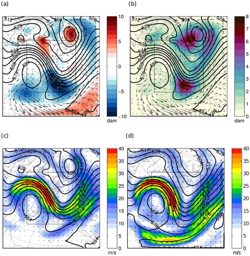
The ECHAM geopotential height field at 500 hPa is averaged over all time steps of the analysis period. Within the domain of the reference set-up (REF), it shows a ridge over the North Atlantic and a trough over Eastern Europe (Fig. 1a–d, contour lines) with a strong north-westerly flow crossing Central Europe and the Alpine region. Upstream of the Alps the wind speeds at 500 hPa reach 40 m/s (Fig. 1a).

Fig. 1. Results of the reference configuration REF based on temporal averages of the analysis period at the 500 hPa level. (a) ECHAM geopotential height (contour lines), wind vectors (arrows) and wind speeds (colours). (b) ECHAM geopotential height (contour lines), ensemble mean wind vector differences (arrows) and wind speed differences (colours) between CCLM and ECHAM. (c) ECHAM geopotential height (contour lines), ensemble mean wind vector differences (arrows) and geopotential height differences (colours) between CCLM and ECHAM. Green rectangles indicate region A (dashed green line) and B (solid green line). (d) ECHAM geopotential height (contour lines), ensemble mean wind vector differences (arrows) and ensemble standard deviation of geopotential height differences between CCLM and ECHAM (colours). The longest vector in b–d is 7.8 m/s.

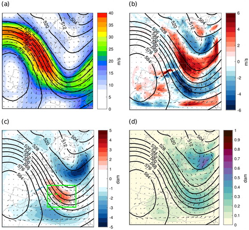
The ensemble mean difference of the wind speeds between CCLM and ECHAM at 500 hPa is calculated using Eq. 4(4) $${\Delta \mathrm{\Phi }}_{\mathit{\text{mean}}}=\frac{1}{N}{\sum }_{i=1}^N\left({\mathrm{\Phi }}_{\mathit{\text{CCLM}},i}-{\mathrm{\Phi }}_{\mathit{\text{ECHAM}}}\right),$$(4) . It shows a reduction of wind speed in the CCLM downstream of the Alps, where the ensemble mean wind speeds in the CCLM are more than 6 m/s lower than in ECHAM (Fig. 1b). This is a reduction of more than 20% compared to ECHAM. This reduction can be explained by orographic drag effects, which appear to be stronger in CCLM. East of the Alps the wind speeds are about 6 m/s higher in CCLM than in ECHAM.

The ensemble mean difference of the geopotential height at 500 hPa between CCLM and ECHAM (${\mathrm{\Delta }Z}_{\mathit{\text{mean}}}$) is calculated using Eq. 4(4) $${\Delta \mathrm{\Phi }}_{\mathit{\text{mean}}}=\frac{1}{N}{\sum }_{i=1}^N\left({\mathrm{\Phi }}_{\mathit{\text{CCLM}},i}-{\mathrm{\Phi }}_{\mathit{\text{ECHAM}}}\right),$$(4) . It shows a tripole pattern similar to the one observed in Becker et al. (2015). A positive geopotential height anomaly of more than 3 dam (decametres) is found in CCLM downstream of the Alps (Fig. 1c). Negative geopotential height anomalies are located north-east and south-west of the positive one. The northerly anomaly is the strongest, reaching −4.75 dam.

The ensemble standard deviation of the geopotential height differences between CCLM and ECHAM (${\mathrm{\Delta }Z}_{std}$) is computed using Eq. 5(5) $${\Delta \mathrm{\Phi }}_{std}=\sqrt{\frac{{\sum }_{i=1}^N{\left[\left({\mathrm{\Phi }}_{\mathit{\text{CCLM}},i}-{\mathrm{\Phi }}_{\mathit{\text{ECHAM}}}\right)-{\Delta \mathrm{\Phi }}_{\mathit{\text{mean}}}\right]}^2}{N-1}}.$$(5) . Compared to ${\mathrm{\Delta }Z}_{\mathit{\text{mean}}}$, the values of ${\mathrm{\Delta }Z}_{std}$ are very low, with local maxima between 0.3 and 0.7 dam in the areas of the three geopotential height anomalies (Fig. 1d). In general, ${\mathrm{\Delta }Z}_{std}$ is about one order of magnitude smaller than ${\mathrm{\Delta }Z}_{\mathit{\text{mean}}}$, suggesting that the geopotential height anomalies are robust features, which only weakly depend on the spin-up time of the CCLM simulations. There is no systematic dependence of the amplitude and spatial structure of the geopotential height anomalies on the spin-up time (not shown).

The ensemble mean wind vector differences between CCLM and ECHAM, representing the SC, are computed using Eq. 1(1) $${\Delta \overrightarrow{v}}_{\mathit{\text{mean}}}=\left(\genfrac{}{}{0pt}{}{\frac{1}{N}{\sum }_{i=1}^N{u}_{\mathit{\text{CCLM}},i}-u_{\mathit{\text{ECHAM}}}}{\frac{1}{N}{\sum }_{i=1}^N{v}_{\mathit{\text{CCLM}},i}-v_{\mathit{\text{ECHAM}}}}\right),$$(1) . As in Becker et al. (2015), they show cyclonic and anticyclonic vortices centred over the negative and positive geopotential height anomalies, respectively (Fig. 1b–d, arrows). The vectors of the SC are aligned approximately parallel to the isolines of ${\mathrm{\Delta }Z}_{\mathit{\text{mean}}}$, suggesting that the SC is close to geostrophic balance. At the southern and eastern boundaries, where the geopotential height anomalies extend towards the buffer zone, the SC shows boundary-parallel flow patterns.

The tripole pattern in the SC and the related geopotential height anomalies, which is shown here only at the 500 hPa layer, extends vertically through the whole troposphere (not shown), as in Becker et al. (2015). The geopotential height anomalies appear above 2 km height and reach up to 15 km. Below 2 km, small-scale anomalies due to direct topographic effects dominate. Above 15 km, where the damping layer begins to have a noticeable effect, the anomalies are close to zero.

3.1.1. Shifted model boundaries

This section focuses on the impact of the location of the individual model boundaries on the SC and the related geopotential height anomalies, which were observed in the reference simulation. Each model boundary is shifted individually by 32 and 64 grid points (576 and 1,152 km) inward and outward, relative to the reference simulation. Inward and outward shifts are noted using minus and plus signs, respectively. For example, W-64 denotes an inward (easterly) shift of the western boundary by 64 grid points.

Figure 2 shows the spatial maps of ${\mathrm{\Delta }Z}_{\mathit{\text{mean}}}$ as well as the SC for shifts of the eastern and western boundary by 64 grid points. Figure 3 shows the same for the northern and southern boundary. Two regions are defined for a more detailed analysis. Region A (green dashed rectangle) is used to compute the area mean of ${\Delta \Vert \overrightarrow{v}\Vert }_{\mathit{\text{mean}}}$ and ${\Delta \Vert \overrightarrow{v}\Vert }_{std}$ downstream of the Alps (note that in S-64 the domain is only partly included in region A). 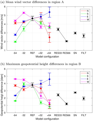Region B (green solid rectangle) is used to identify the positive maximum of ${\mathrm{\Delta }Z}_{\mathit{\text{mean}}}$ and ${\mathrm{\Delta }Z}_{std}$, which is found in the centre of the anticyclonic secondary vortex downstream of the Alpine region. The values obtained for region A and B are summarised for all model configurations in Fig. 4, showing the standard deviations as error bars.

Fig. 2. As Fig. 1c, but for model configurations with shifted (a,c) eastern and (b,d) western model boundaries. Five vertical solid black straight lines (including the outermost boundary) represent the five different locations of each lateral boundary with a distance of 32 grid boxes.

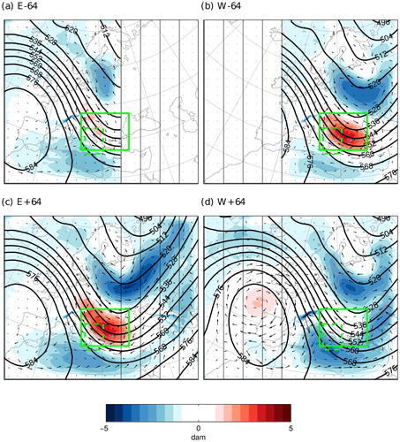
Fig. 3. As Fig. 1c, but for model configurations with shifted (a,b) northern and (c,d) southern model boundaries. Five horizontal solid black straight lines (including the outermost boundary) represent the five different locations of each lateral boundary with a distance of 32 grid boxes.

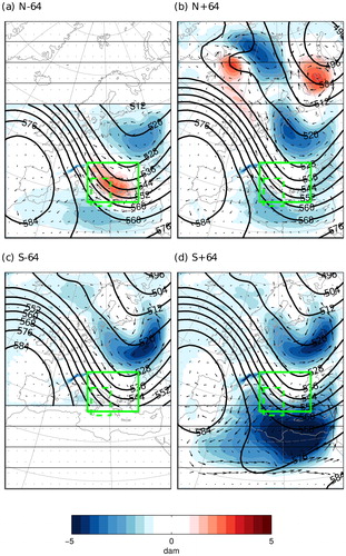
Fig. 4. (a) Area mean of region A of the ensemble mean (points) and standard deviation (error bars) of the norm of the of wind vector differences between CCLM and ECHAM and (b) area maximum of region B of the ensemble mean and standard deviation of the geopotential height differences between CCLM and ECHAM at 500 hPa for different model configurations.

3.1.2. Eastern boundary

An inward shift of the eastern model boundary leads to a reduction of the domain size and brings the boundary closer to the Alps. In E-64, this reduces amplitudes of the geopotential height anomalies below 2.5 dam and leads to a weakened SC, because the CCLM has less space to develop large-scale deviations from the driving data downstream of the Alps (Fig. 2a). If the eastern boundary is shifted outwards and the domain size increases, the amplitude of the positive geopotential height anomaly continuously increases up to 4.5 dam in E + 64 (Fig. 4b). Also, the strength of the SC downstream of the Alps increases continuously from below 3 m/s in E-64 to above 5 m/s in E + 64 (Fig. 4a). The ensemble standard deviations (error bars in Fig. 4) show that the impact of the spin-up time on the geopotential height anomalies and the SC is small compared to the impact of the shifted boundaries. Spatially, in E + 64, the positive geopotential height anomaly and the related anticyclonic vortex in the SC do not extend further eastward than the Black Sea and Turkey. However, the northern negative anomaly and the related cyclonic vortex in the SC extend further eastward, compared to REF, where it was limited by the eastern boundary.

3.1.3. Western boundary

While in the case of the eastern boundary, the strongest SC and geopotential height anomaly were found in the largest domain (E + 64), in the case of the western boundary the anomalies are largest in the smallest domain (W-64, Fig. 2b). Contrary to the eastern boundary, an outward shift of the western boundary from W-64 to W + 64 leads to a continuous reduction of the amplitude of the positive geopotential height anomaly from 4.6 dam to 1.3 dam (Fig. 4a). While the northern negative anomaly shrinks in size, the southern negative anomaly intensifies and extends towards the Black Sea in W + 64 (Fig. 2d). In W + 64, the western boundary extends far into the North Atlantic. The long-wave ridge, which steers the jet stream into Central Europe, is almost completely included within the domain. Within this ridge, an anticyclonic vortex develops in the SC field. Between the centre of this vortex and the Alps, a strong SC crosses the area of France from north to south, which does not occur in the other domains. Apparently, if the western boundary is located further away from the Alps, the RCM has more freedom to modify the flow approaching the Alps. This is sometimes referred to as spatial spin-up (Matte et al., 2017). As a consequence, also the SC pattern downstream of the Alps differs strongly from the other domain configurations, where the inflow boundary is located closer to the Alps. Again, the ensemble spread is relatively small compared to the mean anomalies (Fig. 4).

3.1.4. Northern boundary

While the shift of the western and eastern boundary caused a continuous, almost linear change in the amplitude of the positive geopotential height anomaly, a shift of the northern boundary does not result in such a regular pattern (Fig. 4b). In N-64 and N + 32, the positive geopotential height anomaly is reduced to values below 2 dam and in N + 64 even below 1 dam.

3.1.5. Southern boundary

The shift of the southern boundary has almost no impact on the northern negative geopotential height anomaly, which shows an almost constant amplitude of around −4.5 dam (Fig. 3c and d). On the contrary, the positive and the southern negative geopotential height anomalies depend strongly on the location of the southern boundary. For example, in S + 64, the positive geopotential height anomaly is reduced to 1.1 dam, compared to 3.7 dam in REF (Fig. 4b). Furthermore, the southern negative geopotential height anomaly and the surrounding cyclonic vortex in the SC expand together with the shift of the southern boundary. The negative geopotential height anomaly reaches −5.8 dam in S + 64 in the area of northern Libya. Additionally, the strength of the SC downstream of the Alps is reduced to values below 2 m/s. In S + 64, a strong eastward SC occurs parallel to the southern boundary. Here, the SC reaches more than 12 m/s, while the wind speeds in ECHAM are around 17 m/s in the same region (ECHAM wind speeds are not shown).

3.2. Large domain

In model configuration LARGE, all boundaries are shifted outwards by 125 grid boxes, making the domain approximately twice as large as REF in both x and y directions. The SC in LARGE shows a cyclonic vortex associated with a large negative geopotential height anomaly downstream of the Alps. This negative anomaly has some similarity to the one observed in S + 64, but with an amplitude of more than 10 dam it is approximately twice as strong (Fig. 5a). The amplitudes of the geopotential height anomalies in LARGE are in general much larger than in the model set-ups analysed before. Due to the large domain, the CCLM has more freedom to develop internal variability and deviates stronger from the driving data. This is also shown by the large values of ${\mathrm{\Delta }Z}_{std}$, which reaches 8 dam downstream of the Alps (Fig. 5b). While in REF ${\mathrm{\Delta }Z}_{std}$ was one order of magnitude smaller than ${\mathrm{\Delta }Z}_{\mathit{\text{mean}}}$, in LARGE ${\mathrm{\Delta }Z}_{std}$ and ${\mathrm{\Delta }Z}_{\mathit{\text{mean}}}$ have a similar order of magnitude. This indicates that in LARGE, the results depend strongly on the spin-up time.

Fig. 5. (a) As Fig. 1c, but for model configuration LARGE. (b) As Fig. 1d, but for model configuration LARGE. (c) ECHAM fields as Fig. 1a, but for the domain of model configuration LARGE. (d) Variables as in Fig. 1a, but for the ensemble mean of the CCLM configuration LARGE. The area covered by the model configuration REF is indicated by rectangle in solid black lines.

In the southern part of the LARGE domain, the SC shows an interesting behaviour. While north of approximately 20° latitude the SC vectors are oriented parallel to the isolines of ${\mathrm{\Delta }Z}_{\mathit{\text{mean}}}$, south of 20° latitude (e.g. West Africa) the SC vectors are not parallel but approximately at an angle of 45° to the isolines of the ${\mathrm{\Delta }Z}_{\mathit{\text{mean}}}$, directed from negative towards positive anomalies. The wind speeds in ECHAM are below 5 m/s in this area (Fig. 5c), while the CCLM generates a strong jet with velocities of more 35 m/s (Fig. 5d). Thus, the SC reaches values of more than 30 m/s.

3.3. Horizontal resolution

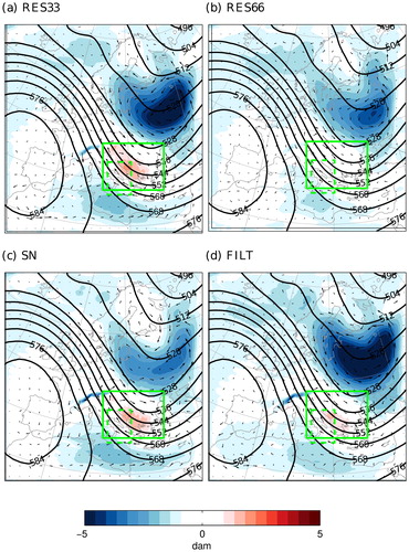
In addition to the REF simulation with a horizontal resolution of 0.165°, two other CCLM set-ups RES33 and RES66 are used, which cover approximately the same domain as REF, but with a horizontal resolution of 0.33° and 0.66°, respectively. The spatial structure of the SC and the geopotential height anomalies in RES33 and RES66 is similar to the spatial structure observed in REF, showing the tripole pattern in the geopotential height anomalies (Fig. 6a and b). However, the intensity of the SC and of ${\mathrm{\Delta }Z}_{\mathit{\text{mean}}}$ depends strongly on the resolution. For example, the strength of the SC in region A decreases with increasing RCM grid size (and decreasing downscaling factor) from 4.5 m/s in REF down to 1.8 m/s in RES66 (Fig. 4a). This can be explained by the coarser resolved topography, which decreases the orographic drag effects compared to REF. Also, the amplitudes of the geopotential height anomalies decrease steadily with increasing grid sizes, except for the northern negative anomaly, which is largest in RES33 (Fig. 6a).

Fig. 6. As Fig. 1c, but for model configurations with different resolutions, spectral nudging and smoothed topography.

3.4. Spectral nudging

In the model set-up SN, the same configuration as in REF is used, but with additional spectral nudging. The spectral nudging is applied to the zonal and meridional wind components above 850 hPa, with the strength of the nudging increasing with height as in von Storch et al. (2000).

The use of spectral nudging reduces the SC and geopotential height anomalies by 30 to 40% compared to REF, whereas the spatial structure of the secondary vortices remains similar (Fig. 6c). In case of the anticyclonic and southern cyclonic secondary vortex, this reduction is comparable to the effect of reducing the resolution to 0.33° degrees, while in case of the northern cyclonic vortex, the reduction is comparable to the 0.66° resolution.

3.5. Filtered topography

The INT2LM, which is a pre-processing tool for the CCLM, provides an option to apply a low-pass filter (Raymond, 1988) to the surface height field before running the CCLM. In the simulation FILT, this filter was applied to smooth the small-scale structure of the CCLM topography, while keeping the large-scale structure similar to REF (the INT2LM configuration is eps_filter =10.000 and norder_filter =5).

The smoothing of the topography leads to a reduction of the amplitude of the positive geopotential height anomaly and the wind vector differences downstream of the Alps by approximately 50%, compared to REF (Fig. 4a and b). In contrast, the spatial structure of the SC and the amplitude of the northern negative geopotential height anomaly are not strongly affected by the smoothing (Fig. 6d). Thus, the impacts of a smoothed topography on the SC are comparable to the impacts of a reduced model resolution.

4. Discussion

Becker et al. (2015) have shown that SCs exist in the climatologies of RCM simulations relative to the driving data prescribed at the lateral boundaries. They argue that the SC is caused by mass flux modifications within the RCM domain, which cannot exit the domain due to the prescribed boundary conditions. Instead, these modifications have to be balanced within the area of the domain and form closed secondary vortices. It was supposed that the location of the RCM boundaries would have a large impact on the characteristics of the SC, also in the inner part of the model domain.

Here, we performed a series of RCM ensemble simulations with different model configurations, including successive shifts of the individual model boundaries, which were compared to a reference configuration. For the simulations, a time period of 108 h was selected, which is characterised by a persistent north-westerly flow crossing the Alps, leading to a pronounced anticyclonic SC, related to a positive geopotential height anomaly downstream of the Alps. For each model configuration, an ensemble of five RCM simulations with different spin-up times prior to the analysis period was computed.

It was shown that the location of each of the four individual lateral boundaries has a large impact on the shape and amplitude of the SC and the related geopotential height anomalies. However, the way the model reacted to shifts of the boundaries was different for each of the four boundaries. In the investigated configurations, an eastward extension of the domain leads to a systematic increase of the amplitude of the anticyclonic circulation anomaly downstream of the Alps. In case of the other boundaries, an outward extension of the domain leads to decreasing amplitudes of the anomaly. The southward extension of the domain leads to the appearance of a dominating cyclonic circulation anomaly that, apparently, suppressed the anticyclonic circulation observed before. In general, the impact of the boundary location on the amplitude and structure of the SC was relatively large. In fact, the changes of the SC induced by the shifting of the boundary had the same order of magnitude as the SC itself. In contrast, the impact of the spin-up time on the amplitude and structure of the SC was relatively small, that is on average one order of magnitude smaller than the SC itself.

The downscaling factor of the reference model set-up was 11.4, which is relatively large, but still within the range suggested by Denis et al. (2003). In practice, much higher downscaling factors are used, as for example in the EURO-CORDEX project (Jacob et al., 2014). Our simulations with different RCM resolutions showed that, in general, a smaller downscaling factor (that means a coarser RCM resolution) leads to a weaker SC with smaller geopotential height anomalies. This can be explained by a reduction of the orographic drag effect with decreasing RCM resolution. The experiment with filtered topography showed that the removal of small-scale topography weakens the anticyclonic secondary vortex downstream of the Alps, similar to a reduced RCM resolution.

In this work, a realistic setting was chosen as a first step, to show the significant impact of the model boundaries on the SC. However, the different factors contributing the characteristics of the SC are difficult to determine and to separate in an RCM setting using the full model with realistic topography. Furthermore, other systematic biases, for example caused by the parameterisation schemes, could be superimposed to the signal of the SC. In future work, idealised test cases with simplified model set-ups could help to separate the impacts of boundary conditions, topography, dynamics and parameterisations on the SC. For example, this could include simulations with idealised topography. As shown in Becker et al. (2015), the shape of the SC depends strongly on the large-scale flow condition. In this work, we focus on one single time period with a specific flow conditions over Europe. One can expect that the amplitude and spatial pattern of the SC are different for other large-large scale flow conditions. In general, large-scale biases are common in RCMs and they occur in different variables at different vertical levels (e.g. Jaeger et al., 2008). These large-scale biases in RCMs are often attributed to the parameterisation schemes (Jacob et al., 2007; Giorgi et al., 2012). For example, in winter a negative bias of total cloud cover and total precipitation was found in central and eastern Europe in CCLM simulations (Jaeger et al., 2008). As precipitation and cloud cover depends strongly on the large-scale circulation (e.g. Lorenzo et al., 2008), we suspected relevant impacts of the SC on these parameterised variables. Therefore, we made additional analyses of precipitation and cloud cover and found mostly small and rather random changes with changing boundary locations (not shown). We found no evidence for a relationship of these changes with the more systematic changes in circulation discussed earlier. However, this could be due to the relatively small ensemble size, which was large enough to generate robust results for the large-scale circulation, but might not be sufficient to capture a relationship with precipitation, which is characterised by a higher randomness and spatial variability.

The domain of model configuration LARGE is comparable to domain sizes used in so-called Big-Brother Experiments (BBE; Denis et al., 2002; Denis et al., 2003; Koltzow et al., 2008). The BBE, as described in Denis et al. (2002), is a ‘perfect-prognosis’ approach. First, a reference climate is generated by running a large-domain high-resolution RCM simulation (called the Big-Brother). The Big-Brother is degraded by filtering small scales that are commonly unresolved in GCMs. The filtered Big-Brother is used to drive a nested RCM simulation (the Little-Brother) with a smaller domain, but with the same resolution as the Big-Brother. If the Little-Brother is able to reproduce the small scales in the unfiltered Big-Brother, this can be declared as added value. The differences between the Little-Brother and the unfiltered Big-Brother can be directly attributed to the nesting and downscaling technique. It should be mentioned here that the specific BBE approach is not adequate to study the SC. The SC arises in our RCM simulations, because small-scale topography has an impact on the large-scale flow. In our GCM, the impact of small-scale topography on the large-scale flow is parameterised and apparently not as strong as in our RCM, which leads to the large-scale circulation anomalies. However, in the Big-Brother (both filtered and unfiltered), the impact of small-scale topography on the large-scale flow is already captured, because it runs at the same high resolution as the Little-Brother. Thus, the conditions that cause the SC are not present in the BBE setting.

5. Conclusions

We showed that the structure and amplitude of large-scale SCs, which occur in one-way nested RCM simulations relative to the driving data, strongly depend on the location of the lateral boundaries. These SCs can be regarded as a superposition of ‘desired’ and ‘undesired’ effects. The desired effect of RCMs, usually named ‘added value’, is a more realistic representation of small-scale effects on the atmospheric conditions, for example the impacts of a higher resolved topography on the large-scale flow. On the other hand, undesired effects or, in other words, model artefacts are caused for example by the presence of the lateral boundaries in an RCM. It is often (implicitly) assumed that the lateral boundaries of an RCM cause artefacts mainly within a limited area in the outer part of the domain, which can be handled by excluding a certain amount of grid boxes from the analysis. This work shows, however, that the location of the lateral boundaries can affect the circulation within the whole model domain. There is no clear systematic dependency between the location of the boundaries and the structure, amplitude and sign of the anomalies. But, in general, the impact of the boundary location on the anomalies is on the same order of magnitude as the amplitude of the anomalies themselves. The largest regional anomalies found in the different investigated configurations amounted more than 30 m/s in horizontal wind speeds at the 500 hPa level, occurring in the largest domain of the regional model. It should be noted that shifts in the inflow and outflow boundary affect the SC with a similar magnitude. Thus, boundary effects propagate both downstream and upstream through the model domain.

In summary, this article clearly points out that significant large-scale anomalies in both wind speed and geopotential heights are caused by using the one-way nesting technique with prescribed boundary conditions. As expected, the anomalies were reduced by applying a smoothed orography, spectral nudging or a coarser resolution of the RCM, but they were still present in all of these cases. Since alternative approaches for dynamical downscaling (e.g. two-way nesting) are often not feasible, in many cases one-way nesting is still the most appropriate option. However, we recommend taking into account the uncertainty arising from the specific choice of the RCM domain. This can be achieved by systematically testing and comparing the impact of different boundary locations on the simulation results. This is particularly relevant when simulating specific case studies with domains including complex topography and strong orographic forcing, because such conditions may lead to strong SCs. That the use of domain shifting techniques is a valuable tool for estimating uncertainties in RCM ensemble simulations, has been shown in several studies (e.g. Pardowitz et al., 2016; Mazza et al., 2017; Noyelle et al., 2018).

Given the potential relevance of the induced anomalies for regional climate and climate change studies, the characteristics of the SC should be analysed in different RCMs. Furthermore, we suggest to explore the mechanisms of the SC and of their implications using model set-ups that are more idealised than those in the present study.

Acknowledgements

We thank the CLM-Community for the support and for making available the CCLM source code. We would also like to acknowledge the high-performance computing service of the ZEDAT of the Freie Universität Berlin for providing allocations of computing time. We thank the editor and two anonymous reviewers for their comments, which helped us to improve the manuscript.

Disclosure statement

No potential conflict of interest was reported by the authors.

Additional information

Funding

This work was supported by the Helmholtz Association in the framework of the Helmholtz Graduate Research School for Explorative Simulation in Earth Sciences (GEOSIM) under Grant VH-KO-408, which is gratefully acknowledged.

References

- Becker, N., Ulbrich, U. and Klein, R. 2015. Systematic large-scale secondary circulations in a regional climate model. Geophys. Res. Lett. 42, 4142–4149. DOI: 10.1002/2015GL063955.
- Bhaskaran, B., Jones, R. G., Murphy, J. M. and Noguer, M. 1996. Simulations of the Indian summer monsoon using a nested regional climate model: domain size experiments. Clim. Dynam. 12, 573–587. DOI: 10.1007/BF00216267.
- Broccoli, A. J. and Manabe, S. 1992. The effects of orography on midlatitude northern hemisphere dry climates. J. Climate. 5, 1181–1201. DOI: 10.1175/1520-0442(1992)005 < 1181:TEOOOM>2.0.CO;2.
- Costa, A. C., Santos, J. A. and Pinto, J. G. 2012. Climate change scenarios for precipitation extremes in Portugal. Theor. Appl. Climatol. 108, 217–234. DOI: 10.1007/s00704-011-0528-3.
- Davies, H. C. 1976. A lateral boundary formulation for multi-level prediction models. Q. J. Roy. Meteor. Soc. 102, 405–418.
- Denis, B, Laprise, R., Caya, D. and Côté, J. 2002. Downscaling ability of one-way nested regional climate models: the big-brother experiment. Clim. Dyn. 18, 627–646. DOI: 10.1007/s00382-001-0210-0.
- Denis, B., Laprise, R. and Caya, D. 2003. Sensitivity of a regional climate model to the resolution of the lateral boundary conditions. Clim. Dyn. 20, 107–126. DOI: 10.1007/s00382-002-0264-6.
- Diaconescu, E. P. and Laprise, R. 2013. Can added value be expected in RCM-simulated large scales? Clim. Dyn. 41, 1769–1800. DOI: 10.1007/s00382-012-1649-9.
- Doms, G., Förstner, J., Heise, R., Herzog, H.-J., Mironov, D. and co-authors. 2011. A Description of the Nonhydrostatic Regional COSMO Model – Part II: Physical Parameterization. Deutscher Wetterdienst, Offenbach, Germany.
- Feser, F., Rockel, B., von Storch, H., Winterfeldt, J. and Zahn, M. 2011. Regional climate models add value to global model data: a review and selected examples. Bull. Amer. Meteor. Soc. 92, 1181–1192. DOI: 10.1175/2011BAMS3061.1.
- Giorgi, F., Coppola, E., Solmon, F., Mariotti, L., Sylla, M. B. and co-authors. 2012. RegCM4: model description and preliminary tests over multiple CORDEX domains. Clim. Res. 52, 7–29. DOI: 10.3354/cr01018.
- Goswami, P., Shivappa, H. and Goud, S. 2012. Comparative analysis of the role of domain size, horizontal resolution and initial conditions in the simulation of tropical heavy rainfall events. Met. Apps. 19, 170–178. DOI: 10.1002/met.253.
- Hollweg, H. D., Boehm, U., Fast, I., Hennemuth, B. Keuler, K. and co-authors. 2008. Ensemble simulations over Europe with the regional climate model CLM forced with IPCC AR4 global scenarios. M & D Tech. Rep. 3, 154.
- Jacob, D., Bärring, L., Christensen, O. B., Christensen, J. H., De Castro, M, and co-authors. 2007. An inter-comparison of regional climate models for Europe: model performance in present-day climate. Clim. Chang. 81, 31–52. DOI: 10.1007/s10584-006-9213-4.
- Jacob, D., Petersen, J., Eggert, B., Alias, A., Christensen, O. B. and co-authors. 2014. EURO-CORDEX: new high-resolution climate change projections for European impact research. Reg. Environ. Change 14, 563–578. DOI: 10.1007/s10113-013-0499-2.
- Jaeger, E. B., Anders, I., Lüthi, D., Rockel, B., Schär, C. and co-authors. 2008. Analysis of ERA40‐driven CLM simulations for Europe. Metz. 17, 349–367. DOI: 10.1127/0941-2948/2008/0301.
- Jones, R. G., Murphy, J. M. and Noguer, M. 1995. Simulation of climate change over Europe using a nested regional-climate model. I: Assessment of control climate, including sensitivity to location of lateral boundaries. QJ. Royal Met. Soc. 121, 1413–1449. DOI: 10.1002/qj.49712353802.
- Jungclaus, J. H., Keenlyside, N., Botzet, M., Haak, H., Luo, J.-J. and co-authors. 2006. Ocean circulation and tropical variability in the coupled model ECHAM5/MPI-OM. J. Climate 19, 3952–3972. DOI: 10.1175/JCLI3827.1.
- Kljun, N., Sprenger, M. and Schär, C. 2001. Frontal modification and lee cyclogenesis in the Alps: a case study using the ALPEX reanalysis data set. Meteorol. Atmos. Phys. 78, 89–105. DOI: 10.1007/s007030170008.
- Koltzow, M., Iversen, T. and Haugen, J. E. 2008. Extended big-brother experiments: the role of lateral boundary data quality and size of integration domain in regional climate modelling. Tellus A 60, 398–410. DOI: 10.1111/j.1600-0870.2008.00309.x.
- Kunz, M., Mohr, S., Rauthe, M., Lux, R. and Kottmeier, C. 2010. Assessment of extreme wind speeds from regional climate models-part 1: estimation of return values and their evaluation. Nat. Hazards Earth Syst. Sci. 10, 907. DOI: 10.5194/nhess-10-2010.
- Larsen, M. A. D., Thejll, P., Christensen, J. H., Refsgaard, J. C. and Jensen, K. H. 2013. On the role of domain size and resolution in the simulations with the HIRHAM region climate model. Clim. Dyn. 40, 2903–2918. DOI: 10.1007/s00382-012-1513-y.
- Lorenzo, M. N., Taboada, J. J. and Gimeno, L. 2008. Links between circulation weather types and teleconnection patterns and their influence on precipitation patterns in Galicia (NW Spain). Int. J. Climatol. 28, 1493–1505. DOI: 10.1002/joc.1646.
- Matte, D., Laprise, R., Thériault, J. M. and Lucas-Picher, P. 2017. Spatial spin-up of fine scales in a regional climate model simulation driven by low-resolution boundary conditions. Clim. Dyn. 49, 563–574. DOI: 10.1007/s00382-016-3358-2.
- Mazza, E., Ulbrich, U. and Klein, R. 2017. The tropical transition of the October 1996 medicane in the western Mediterranean Sea: a warm seclusion event. Mon. Wea. Rev. 145, 2575–2595. DOI: 10.1175/MWR-D-16-0474.1.
- Miguez-Macho, G., Stenchikov, G. L. and Robock, A. 2004. Spectral nudging to eliminate the effects of domain position and geometry in regional climate model simulations. J. Geophys. Res.-Atmos. 109, D13104. DOI: 10.1029/2003JD004495.
- Noyelle, R., Ulbrich, U., Becker, N. and Meredith, E. P. 2018. Assessing the impact of SSTs on a simulated medicane using ensemble simulations. Nat. Hazards Earth Syst. Sci. Discuss. DOI: 10.5194/nhess-2018-230, in review.
- Pardowitz, T., Befort, D. J., Leckebusch, G. C. and Ulbrich, U. 2016. Estimating uncertainties from high resolution simulations of extreme wind storms and consequences for impacts. Metz. 25, 531–541. DOI: 10.1127/metz/2016/0582.
- Radu, R., Déqué, M. and Somot, S. 2008. Spectral nudging in a spectral regional climate model. Tellus A 60, 898–910. DOI: 10.1111/j.1600-0870.2008.00341.x.
- Raymond, W. H. 1988. High-order low-pass implicit tangent filters for use in finite area calculations. Mon. Wea. Rev. 116, 2132–2141. DOI: 10.1175/1520-0493(1988)116 < 2132:HOLPIT >2.0.CO;2.
- Reyer, C., Lasch-Born, P., Suckow, F., Gutsch, M., Murawski, A. and co-authors. 2014. Projections of regional changes in forest net primary productivity for different tree species in Europe driven by climate change and carbon dioxide. Ann. Forest Sci. 71, 211–225. DOI: 10.1007/s13595-013-0306-8.
- Rockel, B., Castro, C. L., Pielke, R. A., V., Storch, H. and Leoncini, G. 2008. Dynamical downscaling: assessment of model system dependent retained and added variability for two different regional climate models. J. Geophys. Res.-Atmos. 113, D21107. DOI: 10.1029/2007JD009461.
- Roeckner, E., Brokopf, R., Esch, M., Giorgetta, M., Hagemann, S. and co-authors. 2006. Sensitivity of simulated climate to horizontal and vertical resolution in the ECHAM5 atmosphere model. J. Climate. 19, 3771–3791. DOI: 10.1175/JCLI3824.1.
- von Storch, H., Langenberg, H. and Feser, F. 2000. A spectral nudging technique for dynamical downscaling purposes. Mon. Wea. Rev. 128, 3664–3673. DOI: 10.1175/1520-0493(2000)128h3664:ASNTFDi2.0.CO;2.