Gaussian approximations in filters and smoothers for data assimilation

Abstract

We present mathematical arguments and experimental evidence that suggest that Gaussian approximations of posterior distributions are appropriate even if the physical system under consideration is nonlinear. The reason for this is a regularizing effect of the observations that can turn multi-modal prior distributions into nearly Gaussian posterior distributions. This has important ramifications on data assimilation (DA) algorithms in numerical weather prediction because the various algorithms (ensemble Kalman filters/smoothers, variational methods, particle filters (PF)/smoothers (PS)) apply Gaussian approximations to different distributions, which leads to different approximate posterior distributions, and, subsequently, different degrees of error in their representation of the true posterior distribution. In particular, we explain that, in problems with ‘medium’ nonlinearity, (i) smoothers and variational methods tend to outperform ensemble Kalman filters; (ii) smoothers can be as accurate as PF, but may require fewer ensemble members; (iii) localization of PFs can introduce errors that are more severe than errors due to Gaussian approximations. In problems with ‘strong’ nonlinearity, posterior distributions are not amenable to Gaussian approximation. This happens, e.g. when posterior distributions are multi-modal. PFs can be used on these problems, but the required ensemble size is expected to be large (hundreds to thousands), even if the PFs are localized. Moreover, the usual indicators of performance (small root mean square error and comparable spread) may not be useful in strongly nonlinear problems. We arrive at these conclusions using a combination of theoretical considerations and a suite of numerical DA experiments with low- and high-dimensional nonlinear models in which we can control the nonlinearity.

Keywords:

• data assimilation
• Gaussian approximation
• ensemble Kalman filter
• particle filter
• variational data assimilation

1. Introduction

Probabilistic geophysical state estimation uses Bayes’ rule to merge prior information about the system’s state with information from noisy observations. Gaussian approximations to prior and posterior distributions in geophysical state estimation are widely used, e.g. in ensemble Kalman filters (EnKF, see, e.g. Evensen, 2006; Tippet et al., 2003) or variational methods (see, e.g. Talagrand and Courtier, 1987; Poterjoy and Zhang, 2015). Application of Gaussian approximations to different objects in different DA algorithms (ensemble Kalman filters/smoothers, variational methods, particle filters (PF)/smoothers (PS)) leads to different approximate posterior distributions, and, subsequently, different degrees of error in their representation of the true posterior. Therefore, not all Gaussian approximations are equal. We explore the use of Gaussian approximations in different DA algorithms using a combination of theoretical considerations and numerical experiments in which we can control the nonlinearity. Our focus is on ramifications of our findings on contemporary DA algorithms in numerical weather prediction (NWP), where the goals is to find an initial condition for a forecast that can be made in real time.

We consider and contrast smoothing algorithms, which estimate the state before observation time, and filtering algorithms, which estimate the state at (or after) observation time. Mathematical arguments and numerical experiments suggest that, within identical problem setups, Gaussian approximations in a smoother can be appropriate even if the model is nonlinear and the filtering prior is not at all Gaussian (e.g. multi modal). We find that this effect arises in regimes of ‘medium’ nonlinearity due to a regularizing effect of the observations (see Bocquet, 2011; Metref et al., 2014; and Section 3 for definitions of mild, medium and strong nonlinearity). In this regime, PS and variational methods tend to outperform the EnKF, while PF require substantially larger numbers of ensemble members to be competitive (even when localized with contemporary methods, see also Poterjoy et al., 2018). In short, the reasons are that (i) smoothers make use of nearly Gaussian smoothing priors and posteriors, while PFs make no assumption about the underlying problem structure even though, in this situation, exploring near Gaussianity is beneficial; (ii) the EnKF implicitly makes a Gaussian approximation of a filtering prior, which, in the regime of medium nonlinearity, is less amenable to Gaussian approximation than the smoothing prior and posterior.

The examples suggest that a fully non-Gaussian approach (e.g. the PF) is worthwhile only if Gaussian approximations to posterior distributions are not appropriate. This happens, for example, if posterior distributions are multi-modal and/or have long and heavy tails. In this case, large ensemble sizes are needed for accurate probabilistic inference. Moreover, state estimation by an (approximate) posterior mean is not meaningful in this situation and computing root mean squared errors (RMSE) and average standard deviations (spread) may be insufficient to assess the performance of a DA algorithm in a strongly nonlinear problem. Thus, the usual indicators of performance of a DA algorithm need to be re-evaluated in strongly nonlinear problems.

High-dimensional problems in NWP require localization. Generally, localization means to reduce errors due to a small ensemble size. In NWP, localization often means to delete ensemble based covariances that suggest unphysical long-range correlations. Localization is well-understood in the EnKF, see, e.g. Hamill et al. (2001); Houtekamer and Mitchell (2001), but localization of PFs is less straightforward and is a current research topic, see, e.g. Lei and Bickel (2011); Reich (2013); Penny and Miyoshi (2015); Tödter and Ahrens (2015); Lee and Majda (2016); Poterjoy (2016); Poterjoy and Anderson (2016); Poterjoy et al. (2017, 2018); Robert and Künsch (2017); Farchi and Bocquet (2018). The various localization techniques proposed over the past years introduce errors and biases, which at this point in time, are not fully understood. We provide numerical examples where additional errors caused by localization of the PF are more severe than errors due to Gaussian approximations in PS.

Metref et al. (2014) also discuss the importance of choosing the appropriate DA algorithm based on the degree of nonlinearity of the model. In fact, our paper can be viewed as an extension of the work by Metref et al. (2014): in addition to considering mild, medium and strong nonlinear test cases, we describe the regularizing effects of observations, discuss the importance of subtle differences between filters and smoothers in problems with medium nonlinearity, and consider advantages and disadvantages of Gaussian approximations compared to localized PFs in high-dimensional problems. There are also connections of our work to iterative ensemble smoothers, recently reviewed by Evensen (2018), as well as the work on iterative ensemble Kalman filters and smoothers, see, e.g. Sakov et al. (2012); Bocquet and Sakov (2013, 2014); Bocquet (2016). In these references, it was found that smoothers can outperform filters and that RMSE can be small even if the smoothers do not sample the ‘true’ posterior distribution. Our work, the numerical examples and the mathematical formulations, corroborate these two points.

2. Background

2.1. Notation, problem setup and assumptions

We set up the notation used throughout this paper and state our assumptions. We use bold face lower case for vectors, bold face capital letters for matrices and italic lower case for scalars. We use N with an index to denote dimension. For example, $N_{\mathrm{x}}$ is the dimension of the vector $\mathbf{x}.$ $N_{\mathrm{e}}$ is ensemble size. The $N_{\mathrm{x}}$ components of a vector $\mathbf{x}$ are denoted by ${[\mathbf{x}]}_j,j=1,\dots ,N_{\mathrm{x}}.$ We write ${\mathbf{I}}_{N_{\mathrm{x}}}$ for the $N_{\mathrm{x}}\times N_{\mathrm{x}}$ identity matrix and $\mathbf{x}\sim \mathcal{N}(\mathbf{m},\mathbf{A})$ for an $N_{\mathrm{x}}$-dimensional Gaussian random vector $\mathbf{x}$ whose mean is $\mathbf{m}$ and whose covariance matrix is $\mathbf{A}.$ We use the shorthand notation ${\mathbf{y}}_{1:n}$ for the set of vectors $\{{\mathbf{y}}_1,\dots ,{\mathbf{y}}_n\}.$

We consider numerical models of the form (1) $${\mathbf{x}}_n=\mathcal{M}\left({\mathbf{x}}_{n-1}\right),$$(1) where $\mathcal{M}:{\mathcal{R}}^{N_{\mathrm{x}}}\to {\mathcal{R}}^{N_{\mathrm{x}}}$ is a function connected to the numerical model and $n=1,2,3,\dots$ is a time index. The observations are (2) $${\mathbf{y}}_n=\mathbf{H}{\mathbf{x}}_n+{\eta }_n,\hspace{1em}{\eta }_n\sim \mathcal{N}(0,{\mathbf{R}}_n),$$(2) where $\mathbf{H}$ is a $N_{\mathrm{y}}\times N_{\mathrm{x}}$ matrix and where R_n are $N_{\mathrm{y}}\times N_{\mathrm{y}}$ symmetric positive definite covariance matrices. Note that the observation error covariance can change over time and that the function $\mathcal{M}$ may involve running a discretized numerical model for several time steps. Thus, our assumptions can be summarized as

1. deterministic model;

2. linear observation function;

3. Gaussian observation errors.

Our assumptions are met by many ‘test-problems’ in the DA literature and are perhaps not too far from NWP reality.

2.2. Probability distributions in filters and smoothers

We define the distributions that arise when a DA algorithm is configured as a filter or a smoother. A filter estimates the state at or after observation time while a smoother uses the current observation to estimate a state in the past. Examples of filters include the EnKF or the PF, smoothers include the ensemble Kalman smoother (EnKS) and the PS. We use the term smoother broadly and also interpret a variational or hybrid DA method as a smoother. There are subtle but important differences between filters and smoothers, which have been discussed in many studies. For example, Weir et al. (2013) have shown that the PS collapses less drastically than the PF. The iterative ensemble Kalman filter (IEnKF) and iterative ensemble Kalman smoother (IEnKS), see, e.g. Sakov et al. (2012); Bocquet and Sakov (2013, 2014); Bocquet (2016), and the variational PS (varPS, see Morzfeld et al., 2018) are also based on the idea of exploring subtle differences between smoothing and filtering.

2.2.1. Prior and posterior distributions of a filter

In the Bayesian framework, one way to combine information from the model and observations is through a filtering posterior distribution, viz. (3) $$p_f\left({\mathbf{x}}_n\right|{\mathbf{y}}_{1:n})\propto p({\mathbf{y}}_n\left|{\mathbf{x}}_n\right)p\left({\mathbf{x}}_n\right|{\mathbf{y}}_{1:n-1}).$$(3)

This filtering posterior distribution describes the probability of the state at observation time n, given the observations up to time n and is the object being approximated in, e.g. the EnKF and the PF. Filters estimate the state based on the posterior mean of ${\mathbf{x}}_n|{\mathbf{y}}_{1:n},$ see, e.g. Evensen (2006). We call the distribution $p({\mathbf{x}}_n|{\mathbf{y}}_{1:n-1}),$ which describes the probability of the current state given the past observations, the filtering prior distribution. The filtering prior is the proposal distribution in the ‘standard PF’ (see, e.g. Doucet et al., 2001) and is also used to generate the forecast ensemble in the EnKF. The distribution $p({\mathbf{y}}_n|{\mathbf{x}}_n)$ is a likelihood, describing the probability of the observations given a model state at time n.

2.2.2. Prior and posterior distributions of a smoother

Another way to combine information within a Bayesian framework is to consider the (lag-one) smoothing posterior distribution (4) $$p_s\left({\mathbf{x}}_{n-1}\right|{\mathbf{y}}_{1:n})\propto p({\mathbf{y}}_n\left|{\mathbf{x}}_{n-1}\right)p\left({\mathbf{x}}_{n-1}\right|{\mathbf{y}}_{1:n-1}).$$(4)

The smoothing posterior distribution describes the state at time n – 1 given the observations up to time n. The likelihood, $p({\mathbf{y}}_n|{\mathbf{x}}_{n-1}),$ is equivalent to the likelihood $p({\mathbf{y}}_n|{\mathbf{x}}_n)$ in the filtering posterior distribution since ${\mathbf{x}}_n=\mathcal{M}({\mathbf{x}}_{n-1}),$ i.e. the state at time n is a deterministic function of the state at time n – 1. We emphasize that the smoothing prior, $p({\mathbf{x}}_{n-1}|{\mathbf{y}}_{1:n-1}),$ is equal to the filtering posterior of the previous cycle. For this reason, we will compare the forecast of a smoother with the analysis of a filter in our numerical experiments below (see also Section 5.1).

We note that we only describe smoothing distributions that ‘walk back’ one observation (lag-one smoothing). It is also possible to use a ‘window’ of L > 1 observations in time (lag-L smoothing). The extension is straightforward and we can make our main points with the simpler lag-1 smoothing and, for that reason, do not discuss lag-L smoothing further.

2.2.3. Nonlinearity

We define what we mean by mild, medium and strong nonlinearity:

• Mild nonlinearity: the model is nonlinear, but the filtering prior is nearly Gaussian.

• Medium nonlinearity: the model is nonlinear, the filtering prior is not nearly Gaussian (e.g. multi-modal) but the filtering and smoothing posterior distributions are nearly Gaussian.

• Strong nonlinearity: the model is nonlinear and the filtering and/or smoothing posterior distributions are not nearly Gaussian (e.g. multi-modal).

These definitions align with what is called mild, medium and strong nonlinearity in Bocquet (2011); Metref et al. (2014) in the context of the Lorenz’63 model (see Section 5).

2.3. Numerical DA algorithms

We list the DA algorithms we consider in numerical experiments and point out where Gaussian approximations are used. This will become important in Sections 4 and 5.

2.3.1. Ensemble Kalman filters and smoothers

There are two common implementations of EnKFs, the ‘stochastic’ EnKF and the ‘square root’ EnKF. The stochastic EnKF operates as follows. Given an ensemble at time n – 1 and a new observation at time n, the forecast model is used to generate an ensemble at time n. Assuming the ensemble at time n – 1 is distributed according to the posterior distribution at time n – 1, the forecast ensemble is distributed according to the filtering prior. The forecast mean and forecast covariance are computed from this ensemble and a Kalman step, performed for each ensemble member, transforms the forecast ensemble into an analysis ensemble. Thus, the EnKF makes use of a Gaussian approximation of the filtering prior because higher moments of the filtering prior are not computed. The EnKF analysis ensemble is approximately distributed according to the filtering posterior if the problem is linear and Gaussian. For a discussion of how the EnKF approximates non-Gaussian distributions, see; Hodyss et al. (2016). The square root EnKF computes the analysis ensemble as a linear combination of the prior ensemble, see, e.g. Tippet et al. (2003); Evensen (2006). The computations only consider the forecast mean and covariances, thus also implicitly making Gaussian approximations of the filtering prior. The square root EnKF and the stochastic EnKF are equivalent if the problem is linear and Gaussian, and if, in addition, the ensemble size is infinite. In all other situations (small/finite ensemble size or nonlinear problem), the stochastic EnKF and square root filters lead to (slightly) different results. For that reason, we consider both implementations of the EnKF in the numerical examples below.

The EnKS uses the prior ensemble to compute covariances through time so that the observation at time n can be used to estimate the state at time n – 1. Since only covariances (of the forecast ensemble through time) are used, but higher moments are neglected, some of the nonlinear effects of the numerical model may be lost. The result of an assimilation with the EnKS is an analysis ensemble. In linear problems, the analysis ensemble approximates the smoothing posterior distribution. An approximation of the filtering posterior can be obtained by propagating the analysis ensemble from this smoother to the observation time via the model.

We note that the distribution of the EnKS or EnKF analysis ensembles in nonlinear problems is not fully understood. It is known, however, that the distribution of the analysis ensemble of deterministic and stochastic EnKFs is not the posterior distribution, see, e.g. Hodyss and Campbell (2013a); Posselt et al. (2014). Nonetheless, the goal of data assimilation (DA) is to produce a sensible probabilistic forecast and, therefore, we assess the quality of EnKF and EnKS in the numerical example below by comparing the distributions of their analysis ensembles to the posterior distribution.

2.3.2. Particle filters

The ‘standard’ PF works as follows. Given an ensemble $\left\{{\mathbf{x}}_{n-1}^j\right\},j=1,\dots N_{\mathrm{e}}$ distributed according to the filtering posterior at time n – 1, $p({\mathbf{x}}_{n-1}|{\mathbf{y}}_{1:n-1}),$ one applies the model to each ensemble member to generate a forecast ensemble ${\mathbf{x}}_n^j=\mathcal{M}({\mathbf{x}}_{n-1}^j)$ at time n. For each ensemble member we then compute a weight $w^j\propto p({\mathbf{y}}^n|{\mathbf{x}}_n^j).$ The weights are subsequently normalized so that their sum is equal to one. This weighted ensemble $\{{\mathbf{x}}_n^j,w^j\}$ is distributed according to the filtering posterior distribution at time n, $p({\mathbf{x}}_n|{\mathbf{y}}_{1:n}).$ The weighted ensemble is typically resampled, i.e. ensemble members with a small weight are deleted and ensemble members with a large weight are duplicated. The above steps are then repeated to incorporate new observations. The standard PF is described in more detail in many papers, e.g. in Doucet et al. (2001).

This PF (and many other PFs for that matter) suffer from the curse of dimensionality and ‘collapse’ when the dimension of the problem is large, see, e.g. Bengtsson et al. (2008); Bickel et al. (2008); Snyder et al. (2008); Snyder (2011); Snyder et al. (2015); Morzfeld et al. (2017). This issue can be overcome by localizing the PF (see below).

A second issue is that the PF using a finite number of ensemble members and a deterministic model will collapse over time regardless of the dimension of the problem. The reason is that it is inevitable that a few ensemble members will be deleted during the resampling step at each observation time. This means that the ensemble collapses to a single ensemble member given enough time. Application of ‘jittering’ algorithms can ameliorate this issue. The purpose of jittering is to increase ensemble spread in a way that does not destroy the overall probability distributions. Several strategies for jittering are described in Doucet et al. (2001). In the numerical examples below, we use a very simple jittering strategy that relies on a Gaussian approximation of the filtering posterior. That is, we use the ‘analysis ensemble’ (after resampling) to compute a mean and covariance matrix. The covariance can be localized and inflated as in the EnKF. We then use this Gaussian to draw a new ensemble that is distributed according to the Gaussian approximation of the filtering posterior distribution. This technique is expected to ‘work well’ in problems with mild or medium nonlinearity. We do not claim that the Gaussian resampling we describe here is new or particularly appropriate. It is, however, a simple strategy that is good enough in the examples we consider and that allows us to make our points. We emphasize that this version of the standard PF, which we call the PF-GR (PF with Gaussian replenishing) is not a fully non-Gaussian DA method as it now makes a Gaussian approximation of the posterior.

We also consider localized versions of the PF. Specifically, we use the ‘local PF’ of Poterjoy (2016) which, in addition to the localization, also incorporates a step similar to covariance inflation in the EnKF. We further use another localized PF, which we call the ‘PF with partial resampling and Gaussian replenishing’ (PF-PR-GR). The idea here is to use a localization scheme for the PF that is similar to how localization is done in the local ensemble transform Kalman filter (LETKF), see, e.g. Hunt et al. (2007). The procedure is as follows. As in the PF, the PF-GR, the EnKF or the EnKS, we begin by generating a forecast ensemble ${\mathbf{x}}_n^j=\mathcal{M}({\mathbf{x}}_{n-1}^j).$ For each component of each ensemble member ${[{\mathbf{x}}_n^j]}_i,i=1,\dots ,N_{\mathrm{x}}$ we compute weights $w^j(i)\propto p({\mathbf{y}}_n^{k(i)}|{\mathbf{x}}^j),$ where k(i) defines the observations in the ‘neighborhood’ of ${[{\mathbf{x}}_n^j]}_i.$ In the numerical examples below we consider the case where we use L observations ‘to the right and to the left’ of the ${[{\mathbf{x}}_n^j]}_i,$ where L is a tunable constant (the numerical example is defined on a 1 D spatial domain, see Section 5.3). We then perform resampling for each component ${[{\mathbf{x}}_n^j]}_i,$ independently of all other components, and based on the local weights $w^j(i).$ After cycling through all components of ${\mathbf{x}}_n^j,$ this procedure generates an ‘analysis’ ensemble. We inflate this analysis ensemble using Gaussian replenishing as described above, i.e. we compute the ensemble mean and covariance, localize and inflate the covariance as in the EnKF, and finally generate a new ensemble that is used for the next assimilation cycle. We do not claim that this localization or inflation scheme is optimal in any way or in fact a particularly appropriate way to localize the PF. For example, the independent (partial) resampling of the components of the state may destroy important model balances. Nonetheless, this localization scheme is perhaps a natural attempt to localize PFs (see also Farchi and Bocquet, 2018), is similar to the localized PF of the German Weather Service (DWD, see Potthast et al., 2018) and will help us make our points about localization in connection with Gaussian approximations. Other localization schemes for the PF are described by Lei and Bickel (2011); Reich (2013); Penny and Miyoshi (2015); Tödter and Ahrens (2015); Lee and Majda (2016); Robert and Künsch (2017).

2.3.3. 4D-Var, ensemble of data assimilation (EDA) and variational PS

A variational DA method (4D-var) assumes a Gaussian background, i.e. the smoothing prior $p({\mathbf{x}}_{n-1}|{\mathbf{y}}_{1:n-1})$ is approximated by a Gaussian with mean μ and covariance matrix $\mathbf{B}.$ One then optimizes the cost function (5) $$J=\frac{1}{2}\left|\right|{\mathbf{B}}^{-1/2}(\mu -{\mathbf{x}}_{n-1})|{|}^2+\frac{1}{2}|\left|{\mathbf{R}}^{-1/2}\right({\mathbf{y}}_n-\mathcal{M}\left({\mathbf{x}}_{n-1}\right)\left)\right|{|}^2,$$(5) typically by a Gauss-Newton method. The inverse of the Gauss-Newton approximate Hessian of the cost function at its minimizer is often used to construct a Gaussian approximation of the smoothing posterior.

Ensemble formulations of 4D-var use an ensemble to update the background covariance and background. In the EDA method, this is done as follows, see, e.g. Bonavita et al. (2012). The optimization is done $N_{\mathrm{e}}$ times to generate an ensemble ${\mathbf{x}}_{n-1}^j,j=1,\dots ,N_{\mathrm{e}},$ but during each optimization a perturbed version of the optimization problem is considered. Specifically, to compute ensemble member j, one optimizes the cost function (6) $$J^j=\frac{1}{2}\left|\right|{\mathbf{B}}^{-1/2}({\tilde{\mu }}^j-{\mathbf{x}}_0)|{|}^2+\frac{1}{2}|\left|{\mathbf{R}}^{-1/2}\right({\tilde{\mathbf{y}}}_n^j-\mathcal{M}\left({\mathbf{x}}_0\right)\left)\right|{|}^2,$$(6) where ${\tilde{\mu }}^j$ is a sample from the Gaussian $\mathcal{N}(\mu ,\mathbf{B})$ and where ${\tilde{\mathbf{y}}}_n^j$ is a sample from the Gaussian $\mathcal{N}({\mathbf{y}}_n,\mathbf{R}).$ The ensemble is then propagated to time n by using the numerical model, ${\mathbf{x}}_n^j=\mathcal{M}({\mathbf{x}}_{n-1}^j).$ The ensemble at time n is used to compute an ensemble covariance, which can be localized and inflated. This localized and inflated covariance replaces the background covariance $\mathbf{B}$ for the next cycle. In the numerical examples of Section 5, we update the background mean by propagating the optimizer of the unperturbed optimization problem (5) to time n.

Note that the ensembles (at time n – 1 and at time n), generated by EDA, are not Gaussian. In fact, the method can be viewed as a version of the ‘randomize-then-optimize’ sampler described by Bardsley et al. (2014) or as an iterative smoother, see, e.g. Evensen (2018). The method, however, relies on a Gaussian approximation of the smoothing prior (background mean and covariance). Other ensemble formulations of 4D-var are also possible, but we only consider EDA. For more detail about ensemble formulations of 4D-var and for comparisons of the various methods see, e.g. Buehner (2005); Liu et al. (2008); Kuhl et al. (2013); Lorenc et al. (2015); Poterjoy and Zhang (2015).

We consider the variational particle smoother (varPS) described in Morzfeld et al. (2018). The method assumes a Gaussian smoothing prior (as in EDA) and solves the unperturbed optimization problem (5). We denote the minimizer by ${\mathbf{x}}_{n-1}^{*}$ and the Gauss-Newton approximation of the Hessian of the cost function J, evaluated at ${\mathbf{x}}_{n-1}^{*}$ by $\mathbf{J}.$ The Gaussian proposal distribution of the varPS is given by $q=\mathcal{N}({\mathbf{x}}_{n-1}^{*},{\mathbf{J}}^{-1})$ and samples from it define the ensemble $\left\{{\mathbf{x}}_{n-1}^j\right\},j=1,\dots ,N_{\mathrm{e}}.$ The ensemble is weighted by the ratio of target and proposal distribution, i.e. $w^j\propto \hspace{0.17em}\text{exp}\hspace{0.17em}(-J({\mathbf{x}}_{n-1}^j))/q({\mathbf{x}}_{n-1}^j).$ The weighted ensemble is distributed according to the distribution $p\propto \hspace{0.17em}\text{exp}\hspace{0.17em}(-J({\mathbf{x}}_{n-1}^j)),$ i.e. to an approximation of the smoothing posterior that relies on a Gaussian approximation of the smoothing prior (just as EDA). The weighted or resampled ensemble is then propagated to time n by using the numerical model, ${\mathbf{x}}_n^j=\mathcal{M}({\mathbf{x}}_{n-1}^j).$ The ensemble at time n is used to compute an ensemble covariance that is localized and inflated as in the EnKF. As in EDA, we update the background mean by propagating the optimizer of the unperturbed optimization problem (5) to time n.

In addition to localizing the ensemble covariance at time n, the weights of the varPS have to be localized when the dimension of the problem is large. Alternatively, one can simply neglect the weights, i.e. use the varPS proposal distribution as an approximation of the target distribution. This can give results similar to what one obtains by localizing the weights, as reported by Morzfeld et al. (2018), and is appropriate when the smoothing posterior is nearly Gaussian. We refer to this technique, which essentially amounts to a Laplace approximation of the smoothing posterior, as the varPS-nw (where the nw indicates that ‘no weights’ are used). Finally, we note that the varPS and in particular the varPS-nw has connections with IEnKS (see, e.g. Sakov et al., 2012; Bocquet and Sakov, 2013, 2014; Bocquet, 2016), which are explained in detail in Morzfeld et al. (2018).

2.3.4. Summary

In Table 1, we summarize how the various DA algorithms deploy Gaussian approximations. We remind the reader that all methods require localization and inflation in high-dimensional problems, but this does not affect how the algorithms make use of Gaussian approximations (hence localization is not emphasized in the table).

Table 1. Gaussian approximations in DA algorithms.

	Targeted posterior	Gauss. app. of filtering prior?	Gauss. app. of filtering posterior?	Gauss. app. of smoothing prior?	Gauss. app. of smoothing posterior?
PF	Filtering	No	No	–	–
PF-GR	Filtering	No	Yes	–	–
EnKF	Filtering	Yes	No	–	–
EnKS	Smoothing	–	No	Yes	No
4D-Var	Smoothing	–	No	Yes	Yes/No
EDA	Smoothing	–	No	Yes	No
varPS	Smoothing	–	No	Yes	No
varPS-nw	Smoothing	–	No	Yes	Yes

The “-” means “not applicable”. Smoothing algorithms can produce approximations of the filtering posterior by the smoother ensemble and the numerical model. The resulting representation of the filtering posterior is not Gaussian. For that reason, smoothing algorithms do not utilize Gaussian approximations of the filtering posterior. Whether or not 4D-Var makes a Gaussian approximation of the smoothing posterior depends on its implementation (see text for more detail).

Recall that smoothers and variational methods target the smoothing posterior while filters target the filtering posterior. Smoothers and variational methods, however, can also produce approximations of the filtering posterior because the smoother’s analysis ensemble, at time n – 1, can be propagated to observation time n via the numerical model. If this model is nonlinear, the ensemble at time n is not Gaussian distributed, even if the variational methods makes use of a Gaussian approximation of the smoothing posterior (e.g. the varPS-nw). For that reason, we include in Table 1 that the smoothing algorithms do not utilize Gaussian approximations of the filtering posterior.

Finally, we emphasize that whether or not 4D-Var makes a Gaussian approximation of the smoothing posterior depends on what type of 4D-Var is implemented. In Section 2.3.3, we describe a ‘simple’ 4D-Var that does make a Gaussian approximation of the smoothing posterior (similar to the proposal distribution in the varPS-nw). There are, however, other ways to implement a 4D-Var and these techniques may not require Gaussian approximations of the smoothing posterior. In this paper, we consider EDA as a representative method of this class of 4D-Var techniques, but other methods have also been successfully applied, e.g. Kuhl et al. (2013).

3. Regularization through observations

We discuss basic properties of the various distributions in filters and smoothers. We then show, under simplifying assumptions (including Gaussian observation errors), that observations have a regularizing effect in the sense that multiplication of a non-Gaussian prior distribution by the likelihood leads to a posterior distribution that is amenable to Gaussian approximation. We provide several simple illustrations of these ideas.

3.1. Connections between the distributions of smoothers and filters

First we note that the smoothing prior at the nth cycle, $p({\mathbf{x}}_{1:n-1}|{\mathbf{y}}_{1:n-1}),$ is the filtering posterior of the previous cycle. Since observations reduce variance, i.e. posterior variances are typically smaller than prior variances, this implies that the smoothing prior is likely to have a smaller variance than the filtering prior at the same cycle. Similarly, the smoothing posterior, $p({\mathbf{x}}_{1:n}|{\mathbf{y}}_{1:n+1}),$ includes more observations than the filtering posterior at the same time, $p({\mathbf{x}}_{1:n}|{\mathbf{y}}_{1:n}).$ Thus, the smoothing posterior has smaller variance than the filtering posterior if we assume that more observations lead to greater error reduction and that smaller errors also results in smaller variances. We can make these statements precise under additional simplifying assumptions (see Appendix). 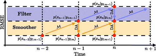Moreover, in a well-tuned DA algorithm, the spread, defined as the square root of the trace of the posterior covariance divided by $N_{\mathrm{x}},$ is comparable to the RMSE. Thus, we can connect the statements about the posterior covariances of filtering and smoothing distributions directly to RMSE: a smaller variance implies a smaller RMSE (and vice versa). This leads to the cartoon in Fig. 1. In addition to illustrating that smoothers operate on lower RMSE levels, Fig. 1 also illustrates how the various distributions are connected. In particular it shows that the filtering posterior at time n is the smoothing prior at the same cycle.

Fig. 1. A simplified schematic diagram of the RMSE of filters and smoothers. Diagonal arrows represent the model and vertical (downward) arrows represent assimilation of observations. The purple and orange regions illustrate the RMSE that the filter and smoother produce.

Intuitively, distributions with a smaller variance are more amenable to Gaussian approximations than distributions with larger variance. For example, a bi-modal distribution with two (identical) well separated modes has a larger variance than a distribution that contains only one of these two modes; a distribution with significant skew typically (but not always) has a larger variance than the same distribution with the skew removed. Our considerations above thus suggest that Gaussian approximations in smoothers are more appropriate than Gaussian approximations in filters. We present simple examples below and further numerical evidence in Section 5 that suggest that this is indeed the case when the nonlinearity is ‘medium’. In strongly nonlinear problems, however, it is generally not true that Gaussian approximations in smoothers are more appropriate than in filters. This is shown by specific numerical examples below and in Section 5.

3.2. Regularization of posterior distributions by observations

We have argued above that observations reduce variance and that a small variance leads to good Gaussian approximations. Here, we make these arguments more precise under the following assumptions. We assume that n = 1 and that $p({\mathbf{x}}_0)$ is Gaussian. Without loss of generality we consider the prior $p({\mathbf{x}}_0)\sim \mathcal{N}(0,{\mathbf{I}}_{N_{\mathrm{x}}}).$ Finally, we assume that the model $\mathcal{M}$ is invertible, i.e. that there exists a function ${\mathcal{M}}^{-1}$ such that ${\mathcal{M}}^{-1}\left(\mathcal{M}(\mathbf{x})\right)=\mathbf{x}.$ Using a change of variables, we can write the filtering prior as (7) $$p\left({\mathbf{x}}_1\right)\propto \hspace{0.17em}\text{exp}\hspace{0.17em}\left(-\frac{1}{2}\left|\right|{\mathcal{M}}^{-1}\left({\mathbf{x}}_1\right)|{|}^2\right)\left|\det \left(\frac{\mathrm{d}{\mathbf{x}}_0}{\mathrm{d}{\mathbf{x}}_1}\right)\right|,$$(7) where $\mathrm{d}{\mathbf{x}}_0/\mathrm{d}{\mathbf{x}}_1$ is the Jacobian matrix of the inverse function ${\mathcal{M}}^{-1}.$ Since $\mathrm{d}{\mathbf{x}}_0/\mathrm{d}{\mathbf{x}}_1={(\mathrm{d}{\mathbf{x}}_1/\mathrm{d}{\mathbf{x}}_0)}^{-1}$ and $\det ({\mathbf{A}}^{-1})=1/\det (\mathbf{A})$ for any nonsingular matrix $\mathbf{A},$ we can re-write the filtering prior as (8) $$p\left({\mathbf{x}}_1\right)\propto \hspace{0.17em}\text{exp}\hspace{0.17em}\left(-\frac{1}{2}\left|\right|{\mathcal{M}}^{-1}\left({\mathbf{x}}_1\right)|{|}^2-\hspace{0.17em}\text{log}\hspace{0.17em}|\det \left(\mathcal{M}\prime \left({\mathcal{M}}^{-1}\left({\mathbf{x}}_1\right)\right)\right)|\right),$$(8) where $\mathcal{M}\prime =\mathrm{d}{\mathbf{x}}_1/\mathrm{d}{\mathbf{x}}_0$ is shorthand notation for the Jacobian of the model $\mathcal{M}.$ The likelihood is (9) $$p\left({\mathbf{y}}_1\right|{\mathbf{x}}_1)\propto \hspace{0.17em}\text{exp}\hspace{0.17em}\left(-\frac{1}{2}\left|\right|{\mathbf{R}}^{-1/2}(\mathbf{H}{\mathbf{x}}_1-{\mathbf{y}}_1)|{|}^2\right)$$(9)

We can thus write the filtering posterior as $p_f({\mathbf{x}}_1|{\mathbf{y}}_1)\propto \hspace{0.17em}\text{exp}\hspace{0.17em}\left(-F_f({\mathbf{x}}_1))\right)$ where (10) $$F_f\left({\mathbf{x}}_1\right)=\frac{1}{2}\left|\right|{\mathbf{R}}^{-1/2}(\mathbf{H}{\mathbf{x}}_1-{\mathbf{y}}_1)|{|}^2+\frac{1}{2}|\left|{\mathcal{M}}^{-1}\right({\mathbf{x}}_1\left)\right|{|}^2+\hspace{0.17em}\text{log}\hspace{0.17em}\left|\det \left(\mathcal{M}\prime \left({\mathcal{M}}^{-1}\left({\mathbf{x}}_1\right)\right)\right)\right|.$$(10)

Note that if F_f is quadratic, then the filtering posterior is Gaussian and vice versa. This happens when the model, $\mathcal{M},$ is linear, so that the second term is quadratic and the third term is a constant. The first term, however, is quadratic even if $\mathcal{M}$ is not linear. This means that (under our assumptions) the observations always have a regularizing effect on the function F_f, making it ‘more quadratic’, which in turn implies that the filtering posterior distribution is ‘more Gaussian’ than the filtering prior. Recall that the observation error covariance matrix $\mathbf{R}$ controls the reduction in variance from filtering prior to posterior, or, equivalently, the strength of the regularization in (10). Large $\mathbf{R}$ lead to a modest reduction in variance and a mild regularizing effect, but with accurate observations and small $\mathbf{R}$ the regularization can be strong and the reduction in variance is large.

So far, we focused on the case of a fixed number of observations, varying their effect on an analysis by varying observation error covariances (because it is mathematically straightforward). One can also consider scenarios in which one holds observation error variances constant and considers large or small numbers of observations. In this case, observation networks with a larger number of observations will lead to more regularization than a observation networks with a smaller number of observations (mathematically, the 2-norm of the observation term in (10) increases with the dimension of $\mathbf{y}$). From a practical perspective, one can expect that a large number of good quality observations result in nearly Gaussian filtering posterior distributions.

An example, suppose that (11) $$\mathcal{M}\left({\mathbf{x}}_0\right)={\mathbf{x}}_0+\epsilon g\left({\mathbf{x}}_0\right),\hspace{1em}{\mathcal{M}}^{-1}\left({\mathbf{x}}_1\right)={\mathbf{x}}_1+\epsilon f\left({\mathbf{x}}_1\right),$$(11) i.e. the model and its inverse are a linear function with an added, small nonlinear term (one can think of the above as a truncation of the Taylor expansions of the nonlinear model and its inverse). Then, equation (10)(10) $$F_f\left({\mathbf{x}}_1\right)=\frac{1}{2}\left|\right|{\mathbf{R}}^{-1/2}(\mathbf{H}{\mathbf{x}}_1-{\mathbf{y}}_1)|{|}^2+\frac{1}{2}|\left|{\mathcal{M}}^{-1}\right({\mathbf{x}}_1\left)\right|{|}^2+\hspace{0.17em}\text{log}\hspace{0.17em}\left|\det \left(\mathcal{M}\prime \left({\mathcal{M}}^{-1}\left({\mathbf{x}}_1\right)\right)\right)\right|.$$(10) becomes (12) $$F_f\left({\mathbf{x}}_1\right)=\frac{1}{2}\left|\right|{\mathbf{R}}^{-1/2}(\mathbf{H}{\mathbf{x}}_1-{\mathbf{y}}_1)|{|}^2+\frac{1}{2}|\left|{\mathbf{x}}_1\right|{|}^2+\epsilon {\mathbf{x}}_1^{T}f\left({\mathbf{x}}_1\right)+\sum _{j=1}^{N_{\mathrm{x}}}\hspace{0.17em}\text{log}\hspace{0.17em}(1+\epsilon {\lambda }_j({\mathbf{x}}_1\left)\right)+O\left({\epsilon }^2\right),$$(12) where ${\lambda }_j({\mathbf{x}}_1)$ are the eigenvalues of the Jacobian of $f({\mathbf{x}}_1).$ Taylor expansion of the eigenvalues ${\lambda }_j({\mathbf{x}}_1),$ which are functions of ${\mathbf{x}}_1$ followed by Taylor expanding the function $\text{log}\hspace{0.17em}(1+x)\approx x-x^2/2+x^3/3+\dots$ leads to a quadratic $F_f({\mathbf{x}}_1)$ with perturbations of size $O(\epsilon ).$ This means that ‘nearly’ linear models, with nonlinearity of order $O(\epsilon ),$ lead to ‘nearly’ Gaussian filtering posterior distributions with F_f being a quadratic with $O(\epsilon )$ higher order terms. This is the regime of mild nonlinearity.

Similarly, we can consider the smoothing posterior which, under our assumptions, can be written as $p_s({\mathbf{x}}_0|{\mathbf{y}}_1)\propto \hspace{0.17em}\text{exp}\hspace{0.17em}\left(-F_s({\mathbf{x}}_0)\right),$ where (13) $$F_s\left({\mathbf{x}}_0\right)=\frac{1}{2}\left|\right|{\mathbf{R}}^{-1/2}\left(\mathbf{H}\mathcal{M}\right({\mathbf{x}}_0)-{\mathbf{y}}_1)|{|}^2+\frac{1}{2}|\left|{\mathbf{x}}_0\right|{|}^2.$$(13)

Note that the regularization is due to the Gaussian prior $p({\mathbf{x}}_0).$ The likelihood adds non-Gaussian effects due to the nonlinearity of the model $\mathcal{M}.$ Recall from Section 3.1 that when we cycle through observations, the filtering posterior, $p({\mathbf{x}}_{n-1}|{\mathbf{y}}_{1:n-1}),$ takes the role of the smoothing prior (see equation (4)(4) $$p_s\left({\mathbf{x}}_{n-1}\right|{\mathbf{y}}_{1:n})\propto p({\mathbf{y}}_n\left|{\mathbf{x}}_{n-1}\right)p\left({\mathbf{x}}_{n-1}\right|{\mathbf{y}}_{1:n-1}).$$(4) ). By our arguments above, we can expect that the filtering posterior can be nearly Gaussian even if the model is nonlinear. This means that the regularization of the smoothing posterior, stemming from the Gaussian prior, is not an artifact of our simplifying assumptions but we can indeed expect that the posterior distribution from a previous cycle has a regularizing effect on the current DA cycle. For the nearly linear model in equation (11)(11) $$\mathcal{M}\left({\mathbf{x}}_0\right)={\mathbf{x}}_0+\epsilon g\left({\mathbf{x}}_0\right),\hspace{1em}{\mathcal{M}}^{-1}\left({\mathbf{x}}_1\right)={\mathbf{x}}_1+\epsilon f\left({\mathbf{x}}_1\right),$$(11) we find, with $\mathbf{H}={\mathbf{I}}_{N_{\mathrm{x}}}$ and $\mathbf{R}={\mathbf{I}}_{N_{\mathrm{x}}},$ that (14) $$F_s\left({\mathbf{x}}_0\right)=\frac{1}{2}\left|\right|{\mathbf{y}}_1-{\mathbf{x}}_0|{|}^2+\frac{1}{2}|\left|{\mathbf{x}}_0\right|{|}^2+\epsilon ·{({\mathbf{y}}_1-{\mathbf{x}}_0)}^{T}g\left({\mathbf{x}}_0\right)+O\left({\epsilon }^2\right).$$(14)

We emphasize that the first two terms are quadratic in ${\mathbf{x}}_0$ and, therefore, these two terms lead to a Gaussian. Thus, mild nonlinearities (small ε) lead to nearly Gaussian posterior distributions.

In summary, we conclude that when a mildly nonlinear model causes a mildly non-Gaussian filtering prior, then Gaussian observation errors and linear observation operators cause a regularization effect that keeps filtering and smoothing posterior distributions nearly Gaussian and, therefore, amenable to Gaussian approximations. Such a regularization by observations can also occur when the nonlinearity of the model is more severe. We provide simple examples of this situation below and provide further numerical evidence of this statement in Section 5.

3.3. Illustrations

We illustrate the regularizing effects of the observations in scalar examples for which we can compute the filtering and smoothing prior and posterior distributions. The nonlinear models ($x_1=\mathcal{M}(x_0)$) we consider are listed in Table 2. For both models, we use an observation y = 0 with Gaussian observation noise of mean zero and standard deviation one. The precise value of the observation y is not important and we use y = 0 because it corresponds to an unperturbed observation of the prior mean. We use Gaussian priors, which are also listed in Table 2. Further shown in Table 2 are the negative logarithm of the filtering prior, $p(x_1),$ filtering posterior, $p_f(x_1|y)$ and smoothing posterior, $p_s(x_0|y)$ (up to an additive constant that is irrelevant). The regularization, coming from the linear observations, is evident from the quadratic terms that appear in the posterior distributions but not in the filtering prior.

Table 2. Filtering prior, filtering posterior and smoothing posterior of two nonlinear examples.

Model #	1	2
Nonlinearity	$x_1=\text{atan}(x_0)$	$x_1=\frac{x_0}{1+x_0},\left|x_0\right|<1$
Prior	$\mathcal{N}(0,1)$	$\mathcal{N}(0,\frac{1}{16})$
$-\hspace{0.17em}\text{log}\hspace{0.17em}(p(x_1))$	$\frac{1}{2}{(\hspace{0.17em}\text{tan}\hspace{0.17em}{x}_1)}^2+2\hspace{0.17em}\text{log}\hspace{0.17em}(\hspace{0.17em}\text{cos}\hspace{0.17em}(x_1))$	$\frac{1}{32}{\left(\frac{x_1}{1-x_1}\right)}^2+2\hspace{0.17em}\text{log}\hspace{0.17em}(1-x_1)$
$-\hspace{0.17em}\text{log}\hspace{0.17em}(p_f(x_1|y))$	$\frac{1}{2}{x}_1^2+\frac{1}{2}{(\hspace{0.17em}\text{tan}\hspace{0.17em}{x}_1)}^2+2\hspace{0.17em}\text{log}\hspace{0.17em}(\hspace{0.17em}\text{cos}\hspace{0.17em}(x_1))$	$\frac{1}{2}{x}_1^2+\frac{1}{32}{\left(\frac{x_1}{1-x_1}\right)}^2+2\hspace{0.17em}\text{log}\hspace{0.17em}(1-x_1)$
$-\hspace{0.17em}\text{log}\hspace{0.17em}(p_s(x_0|y))$	$\frac{1}{2}{x}_0^2+\frac{1}{2}\text{atan}{(x_0)}^2$	$\frac{1}{32}{x}_0^2+\frac{1}{2}{\left(\frac{x_0}{1+x_0}\right)}^2$

The regularizing effects can be illustrated by plotting the distributions in Fig. 2 (blue lines). We also plot a Gaussian approximation (red lines) of each distribution, which we obtain by drawing 10⁶ samples from each distribution and then computing the ensemble mean and ensemble variance. The bin heights of (normalized) histograms of the samples are shown as orange dots. For model #1 ($x_1=\text{atan}(x_0),$ first row in Fig. 2) the observations regularize a multi-modal filtering prior into uni-modal posterior distributions (this also happens in L63, see Section 5.2). When the model is a rational function (model #2, second row in Fig. 2), we observe that the smoothing posterior is ‘almost’ Gaussian even though the filtering prior is not nearly Gaussian.

Fig. 2. Filtering prior (left), filtering posterior (center) and smoothing posterior (right) of two nonlinear models. Top row: $x_1=\text{atan}(x_0).$ Bottom row: $x_1=x_0/(1+x_0),\left|x_0\right|<1.$ Shown are the distributions in blue, the bin heights of histograms obtained from 10⁶ samples as orange dots, and a Gaussian approximation in red.

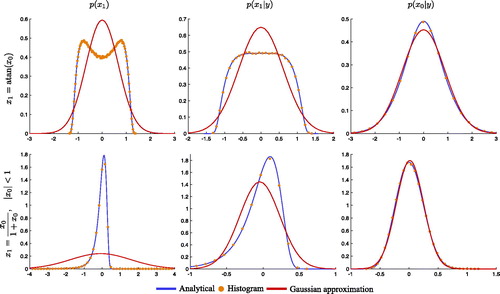
We can quantify the non-Gaussian effects by computing the skewness and excess kurtosis of the three distributions. We compute these quantities from the 10⁶ samples we draw and show our results in Table 3. For model #1, we find that all three distributions are symmetric about the mean and, hence, the skewness is zero. The distribution, however, is not Gaussian and we note that the excess kurtosis is larger for the filtering prior than for the posterior distributions (recall that the excess kurtosis of a Gaussian is equal to zero). For model #2 we find that the two measures of non-Gaussianity are several orders of magnitude larger for the filtering prior than for the posterior distributions. In summary, the two measures of non-Gaussianity (skewness and excess kurtosis) illustrate that the filtering prior is ‘less Gaussian’ than the posterior distributions of a filter or smoother.

Table 3. Skewness and excess kurtosis of filtering prior, filtering posterior and smoothing posterior of four nonlinear examples.

	$x_1=\text{atan}(x_0)$	$x_1=\frac{x_0}{1+x_0},\left|x_0\right|<1$	$x_1=\hspace{0.17em}\text{exp}\hspace{0.17em}(x_0)$	$x_1=\hspace{0.17em}\text{log}\hspace{0.17em}(x_0),x_0>0$
Skewness of $p(x_1)$	$8.30·{10}^{-4}$	–332.57	6.33	–1.54
Skewness of $p(x_1|y)$	$-3.05·{10}^{-4}$	–1.48	1.28	–0.59
Skewness of $p(x_0|y)$	$-5.65·{10}^{-4}$	0.15	–0.49	0.93
Excess kurtosis of $p(x_1)$	–1.228	$2.17·{10}^5$	109.4	4.09
Excess kurtosis of $p(x_1|y)$	–1.06	4.03	2.11	0.41
Excess kurtosis of $p(x_0|y)$	0.36	–0.12	0.18	0.99

The two examples suggest that there are problems for which a Gaussian approximation of the smoothing posterior is more appropriate than a Gaussian approximation of the filtering posterior. Specifically, using a Taylor series around the mode ($x_1=0$), the filtering posterior of model #1 can be written as (15) $$p_f\left(x_1\right|y)=\hspace{0.17em}\text{exp}\hspace{0.17em}(-F_f\left(x_1\right)),\hspace{1em}{F}_f(x_1)=\frac{1}{6}{x}_1^4+\frac{13}{90}{x}_1^6+\cdots .$$(15)

We note the missing quadratic term, which suggests that a Gaussian approximation, which is equivalent to a quadratic approximation of $F_f(x_1)$ is not appropriate. The smoothing posterior distribution, again using Taylor series at the model $x_0=0,$ can be written as (16) $$p_s\left(x_0\right|y)=\hspace{0.17em}\text{exp}\hspace{0.17em}(-F_s\left(x_0\right)),\hspace{1em}{F}_s(x_0)=x_0^2-\frac{1}{3}{x}_0^4+\cdots ,$$(16) which shows that a Gaussian approximation can be valid for small x₀ near the mode. Similar expansions can be done for model #2, but the modes of the distributions are not at $x_1=0$ or $x_0=0,$ which makes the expressions longer and the effects are also less dramatic: both negative logarithms of the posterior distributions have quadratic terms in their Taylor expansions. The non-quadratic terms, however, are larger for the filtering posterior distribution, which demonstrates, just as the measures of non-Gaussianity in Table 3, that the smoothing posterior is more suitable for Gaussian approximations than the filtering posterior.

Another class of problems where a Gaussian approximation of the smoothing posterior may be more appropriate than a Gaussian approximation of the filtering posterior are characterized by numerical models $\mathcal{M}$ which impose constraints on the variable x₁. A simple example is the nonlinearity $x_1=\hspace{0.17em}\text{exp}\hspace{0.17em}(x_0),$ which imposes the constraint that $x_1>0$ so that the conditional random variable $x_1|y$ is also constrained to be positive. Gaussian approximations of $p_f(x_1|y)$ do not (easily) incorporate this constraint. The random variable x₀ as well as the conditional random variable $x_0|y,$ however, are not constrained and, for that reason, Gaussian approximations of the smoothing posterior are appropriate. This can be illustrated by plotting the filtering prior and the posterior distributions in Fig. 3 (top row). We can also compute skewness and excess kurtosis for this example and the results are shown in Table 3. As before, our estimates of skewness and excess kurtosis are based on 10⁶ samples and using the observation y = 0. As the in previous two examples, this numerical experiment indicates that posterior distributions are ‘more Gaussian’ than the filtering prior.

Fig. 3. Filtering prior (left), filtering posterior (center) and smoothing posterior (right) of two nonlinear models. Top row: $x_1=\hspace{0.17em}\text{exp}\hspace{0.17em}(x_0).$ Bottom row: $x_1=\hspace{0.17em}\text{log}\hspace{0.17em}(x_0),x_0>0.$ Shown are the distributions in blue, the bin heights of histograms obtained from 10⁶ samples as orange dots, and a Gaussian approximation in red.

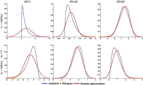
All three examples are characterized by smoothing posteriors that are more amenable to Gaussian approximation than the filtering posteriors. It is however generally not true that the smoothing posterior is always ‘more Gaussian’ than the filtering posterior. A simple example is the inverse of the previous example, i.e. the nonlinearity $x_1=\hspace{0.17em}\text{log}\hspace{0.17em}(x_0).$ We show the filtering prior and the posterior distributions with their Gaussian approximations in Fig. 3. Table 3 also shows the values of skewness and excess kurtosis for this example (based, as before, on 10⁶ samples and using the observation y = 0). The measures of non-Gaussianity indicate that the filtering posterior is ‘more Gaussian’ than the smoothing posterior.

4. Ramifications for numerical DA

In Section 3, we describe the regularizing effect of the observations on posterior distributions and argued that Gaussian approximations of posterior distributions are more appropriate than Gaussian approximations of the filtering prior distribution. We remind the reader of our main conclusions:

1. in problems with medium nonlinearity, observations have a regularizing effect such that posterior distributions (filtering or smoothing) can be nearly Gaussian even if the filtering prior is not nearly Gaussian;

2. when the nonlinearity is strong, the regularizing effect of the observations is mild and posterior distributions are not nearly Gaussian.

We now consider the ramifications of these findings on cycling DA methods, described in Section 2.3, that make use of different Gaussian approximations to different distributions.

4.1. Mild nonlinearity

When nonlinearity is mild, prior and posterior distributions are nearly Gaussian. In this case, one can expect that RMSE and spread of the EnKF/EnKS, variational methods and the PF are comparable. The computational requirements of each algorithm should thus be the main factor for selecting a specific algorithm. The computational cost of an algorithm depends, at least in part, on how much the algorithm can make use of the problem structure (characteristics of the numerical model, observation operators and observation errors). We thus note that the PFs make no assumptions about the problem structure (no Gaussian or linear assumptions). Variational methods (varPS and EDA) and the EnKF/EnKS make Gaussian approximations, which, for mildly nonlinear problems, are indeed valid. Since the PF exploits less problem structure than EnKF/EnKF or a variational method, we expect that the PF is not as effective as the other techniques. Put differently, when the problem really is nearly Gaussian an efficient DA method should make explicit use of that fact; the PFs not exploiting near-Gaussian problem structure in problems with mild nonlinearities is, thus, a drawback. These ideas are conditional on the assumption that the mild deviation from Gaussianity does not have significant effects of increased RMSE or spread.

4.2. EnKF vs. variational DA in problems with medium nonlinearity

In problems with medium nonlinearity, the filtering prior is not nearly Gaussian (e.g. bimodal), but the filtering posterior (smoothing prior) and smoothing posterior are nearly Gaussian. Recall that the EnKF uses a Gaussian approximation of the filtering prior; variational methods (varPS, EDA) assume that the smoothing prior and posterior are Gaussian. Using result (i), we thus expect that variational methods lead to better performance (in terms of RMSE, spread and required ensemble size) than the EnKF when the nonlinearity is medium.

4.3. PF vs. variational DA in problems with medium nonlinearity

Variational methods (varPS and EDA), with localization, exploit near-Gaussian smoothing posterior distributions as well as locality of correlations. Localized PFs exploit local correlation structure but make no additional assumptions. Thus, as in the case of mild nonlinearity, we expect that variational methods are more effective than the PFs in problems with medium nonlinearity because variational methods exploit more of the problem’s structure.

4.4. PF vs. variational DA in problems with strong nonlinearity

Strong nonlinearity leads to filtering and/or smoothing posterior distributions that are not nearly Gaussian (e.g. multi-modal). This means that variational methods (varPS or EDA), which make use of Gaussian approximations of posterior distributions, can be expected to break down. For example, in a multi-modal scenario, the varPS or EDA may represent one of the modes, but fail to represent the others. This could be overcome by more careful optimization (e.g. find several modes, perform local Gaussian approximations at each one and combine the results in a Gaussian mixture model), but we do not pursue these ideas further. The PFs are thus worthwhile in strongly nonlinear problems because the PFs do not rely on Gaussian approximations (of prior or posterior distributions). One should, however, expect larger required ensemble sizes, even if the PFs are localized by contemporary methods. The reason is that even scalar distributions, which are severely non-Gaussian (e.g. multi-modal), require a large ensemble size (hundreds to thousands, see also the conclusions in Poterjoy et al., 2018) to resolve all of the modes and/or any long tails of the distributions. In addition, the required ‘jittering’ must be implemented carefully and, preferably, without Gaussian approximations.

4.5. Filters vs. smoothers

We do not have general results that support that the filtering posterior is ‘more Gaussian’ than the smoothing posterior or vice versa. In DA practice, however, the EnKS is routinely used. In the numerical examples below, we find that the EnKS can yield smaller RMSE than the EnKF (all errors are computed at the same time) in problems with mild or medium nonlinearity. This suggests that, for these examples, the Gaussian approximations in a smoother are more appropriate than the Gaussian approximation of the filtering prior in mild to medium nonlinearity. Some of the examples of Section 3.3, however, show that the opposite can also be true. The numerical illustrations below reveal an interesting secondary result. When nonlinearity is strong, the EnKF leads to smaller RMSE than variational methods. Probabilistic inference based on the EnKF, however, are likely do be unreliable because of inappropriate assumptions (near Gaussian filtering prior).

5. Numerical illustrations

We illustrate the ramifications of our findings on DA algorithms by two numerical examples. We first consider a ‘classical’ low-dimensional example, the L63 model, see Lorenz (1963). Localization is not required for this low-dimensional model (but using localization may further reduce errors). The numerical experiments with L63 can thus be viewed as a benchmark for what one can expect in a best case scenario for high-dimensional problems when the localization is done adequately. The low-dimensional problem and the fact that we do not use (need) localization allows us to compare the PF with the EnKF/EnKS and variational methods in a fair way. On a high-dimensional problem, the PF will collapse unless it is localized, but the localization of the PF is not (yet) fully understood. We address additional difficulties and errors that can arise in the PF due to localization in high-dimensional problems separately by numerical examples with a Korteweg-de-Vries (KdV) equation with one spatial dimension (and state dimension 128). For both models, we perform a series of numerical DA experiments and compare a number of different numerical DA methods.

The results we obtain in our numerical experiments are quantitatively not portable to operational NWP frameworks, where the dimension is significantly larger (10⁸ rather than 3 or 10²) and where additional biases and errors arise because the observations are of the Earth’s atmosphere, not of the numerical model. However, considering low-dimensional models enables us to compare a large number of DA methods in a variety of settings for which we can control the nonlinearity. This is infeasible to do within operational NWP frameworks. We anticipate that the qualitative trends we observe in our simple examples are indicative of what one can expect to encounter in NWP.

5.1. Performance metrics and tuning

All algorithms are implemented with inflation and with localization when required (KdV). We tune localization and inflation parameters for each algorithm and each ensemble size. Throughout this paper, we only present tuned results. The tuning finds the inflation and (when needed) localization parameters that minimize the time averaged RMSE. RMSE at observation time k is defined by (17) $${\text{RMSE}}_k=\sqrt{\frac{1}{N_{\mathrm{x}}}\sum _{j=1}^{N_{\mathrm{x}}}{\left({\left[{\mathbf{x}}_k^t\right]}_j-{\left[{\mathbf{x}}_k^a\right]}_j\right)}^2},$$(17) where ${\mathbf{x}}_k^t$ is the true state and ${\mathbf{x}}_k^a$ is the ‘analysis’ of the DA method we test. For the EnKFs and the PFs, ${\mathbf{x}}_k^a$ is the mean of the analysis ensemble. For the EnKS, ${\mathbf{x}}_k^a$ is the mean of the analysis ensemble at time k – 1, propagated to the observation time k by the model, $\mathcal{M}.$ For the variational methods (EDA and varPS) ${\mathbf{x}}_k^a$ is the minimizer of the cost function (unperturbed in case of EDA) propagated to the observation time k by the model, $\mathcal{M}.$ The spread at observation time k is defined by (18) $${\text{Spread}}_k=\sqrt{\frac{1}{N_{\mathrm{x}}}\text{trace}\left({\mathbf{P}}_a\right)},$$(18) where P_a is the approximate posterior covariance at time k. For the EnKFs and the PFs, P_a is, thus, the covariance of the analysis ensemble. For the EnKS, P_a is computed from the analysis ensemble at time k – 1 propagated to observation time k by the model. Similarly, for EDA and the varPS, P_a is computed as the covariance of the analysis ensemble at time k – 1, propagated to time k by the model.

5.2. Low-dimensional example: L63

We consider the L63 model described in Lorenz (1963). The L63 model is a set of three differential equations (19) $$\frac{\mathrm{d}x}{\mathrm{d}t}=\sigma (y-x),\hspace{1em}\frac{\mathrm{d}y}{\mathrm{d}t}=x(\rho -z)-y,\hspace{1em}\frac{\mathrm{d}z}{\mathrm{d}t}=\mathit{xy}-\beta z,$$(19) where we use the ‘classical’ setting with σ = 10, ρ = 28 and $\beta =8/3.$ We discretize the equations with a fourth order Runge-Kutta (RK) method and use a time step of $\Delta t=0.05.$ The model $\mathcal{M}$ in equation (1)(1) $${\mathbf{x}}_n=\mathcal{M}\left({\mathbf{x}}_{n-1}\right),$$(1) thus represents solving the L63 dynamics, discretized by an RK4 scheme with time step \ $\Delta t$, and run for ΔT time units (equivalently, $\Delta T/\Delta t$ steps). In the numerical experiments below, we consider ΔT between 0.1 and 0.6. As described by Metref et al. (2014) and Bocquet (2011), this corresponds to mild ($\Delta T=0.1$), medium ($0.2\le \Delta T\le 0.4$) and strongly nonlinear ($\Delta T\ge 0.5$) test cases. Following Metref et al. (2014), we focus on observations of all three state variables with observation noise covariance $\mathbf{R}=4{\mathbf{I}}_3.$ The results we obtain with this problem setup, however, are robust and we briefly mention some other problem setups we considered.

Note that we use the time interval between observations to control the nonlinearity to in turn control the non-Gaussianity of prior and posterior distributions. One could also envision other mechanisms for controlling the non-Gaussianity, e.g. by considering different observation networks (less observations lead to more non-Gaussianity) or different observation error covariances (larger error covariances lead to more non-Gaussianity). Our more theoretical considerations, however, are more in line with controlling non-Gaussianity by the time interval between observations and, for that reason, this is the only case we consider here.

5.2.1. Setup, tuning and diagnostics

We consider ‘identical twin’ experiments to test and compare the various DA algorithms described above. For a given time interval between observations, ΔT, we perform a simulation with L63 that serves as the ground truth and then generate observations by perturbing the ground truth with Gaussian noise with covariance $\mathbf{R}.$ Each experiment consists of 1,200 DA cycles. The first 200 cycles are neglected as ‘spin up’.

For each DA algorithm, we tune the inflation and do not use localization (for this reason we do not consider the PF-PR-GR). We use ‘multiplicative prior inflation’, i.e. we multiply the forecast covariance by a scalar. To tune the inflation we consider a number of inflation parameters (ranging from 0.9 to 1.8) and declare the value that leads to the smallest (time averaged) RMSE as the optimal value. Each algorithm is initialized by an ensemble that is generated by a tuned EnKF. This reduces spin-up time, which saves overall computation time of performing the DA experiments because each experiment can be shorter. We also vary the ensemble size for each algorithm. Below we present results we obtained with $N_{\mathrm{e}}=50$ for all algorithms except the PF-GR, for which we use $N_{\mathrm{e}}={10}^3.$ The reason is that larger ensemble sizes do not significantly reduce RMSE. We made little effort to find the ‘minimum’ ensemble size required, but considered ensemble sizes $N_{\mathrm{e}}=20,50,100,200,500,1000.$ We found that $N_{\mathrm{e}}=50$ works well for most algorithms and all ΔT we consider, except the PF-GR, which requires larger $N_{\mathrm{e}}$ (see below for more details).

We compute an average skewness as a quantitative indicator of non-Gaussianity of the filtering prior and filtering/smoothing posterior distributions. We obtain estimates of the skewness by using the PF-GR with ensemble size $N_e={10}^6.$ We used such a large ensemble because computing skewness is noisy and sampling errors are large unless the ensemble size is large. More specifically, at observation time k, we compute the skewness of the x, y and z variables based on the forecast ensemble (filtering prior), and the ensemble distributed according to the smoothing posterior and the ensemble distributed according to the filtering posterior. In this context, it is important to recall that the smoothing prior at the current cycle is the filtering posterior of the previous cycle. We then average the absolute values of the skewness in x, y and z. Using the absolute value is necessary to avoid cancelations in positive or negative skewness. This average absolute values of the skewness, averaged over the variables, is then averaged over the 1,000 DA cycles (after spin-up). The code we used for this paper is available at https://github.com/mattimorzfeld. An animation of the filtering prior and filtering posterior distributions for problems with mild, medium and strong nonlinearity can be found in the supplementary materials.

5.2.2. Results

We plot RMSE as a function of the time interval between observations in the left panel of Fig. 4 and we plot the average skewness of the filtering/smoothing prior and the filtering/smoothing posterior distributions as a function of the time interval between observations in the right panel of Fig. 4. We do not show the spread in the left panel because it is comparable to RMSE for each DA algorithm but the plots are easier to read without the spread. We note that the average skewness increases with the time interval between the observations, indicating that the problem becomes indeed more non-Gaussian (in terms of both prior and posterior distributions) as the time interval between observations becomes larger. Recall, however, that skewness is zero whenever a distribution has symmetry, and therefore small (or even zero) skewness does not imply a Gaussian distribution (see also Section 3.3). We also remind the reader here that the smoothing prior is identical to the filtering posterior and its skewness is indirectly depicted in the right panel of Fig. 4.

Fig. 4. Left: RMSE as a function of the time interval between observations for a fully observed L63 system. Right: average of absolute value of skewness of filtering/smoothing priors and filtering/smoothing posteriors.

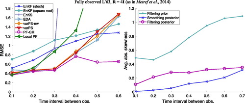
For each DA method, the RMSE increases with the time interval between the observations but at different rates. This difference in the rate of increase of RMSE as the interval between observations increases is a clear factor determining the differences in the methods. It is clear from Fig. 4 that the PF-GR gives the smallest RMSE at any ΔT. The results shown in Fig. 4 are consistent with those reported by Metref et al. (2014). In particular, we note that the RMSE of the PF-GR is comparable with the RMSE of the multivariate rank histogram filter, see Metref et al. (2014). The results we obtain here with the PF-GR are also comparable to the PF used by Metref et al. (2014), which differs from the PF-GR in its inflation (jittering) scheme.

The EnKFs yield a larger RMSE than the PF-GR for all ΔT. The difference in RMSE between the EnKFs and the PF-GR however increases with the time interval between observations. We also note that the square root filter gives a slightly larger RMSE than the stochastic implementation. RMSE of the local PF is comparable to that of the PF-GR when $0.1\le \Delta T\le 0.2,$ but its performance degrades when the time interval is increased. Since we do not make use of the localization of this algorithm (we set the localization radius to be large), the poor performance for large ΔT indicates that the inflation used by the local PF is not ideal for problems with medium nonlinearity. This issue is addressed in Poterjoy et al. (2018), where new inflation strategies of the local PF are discussed.

The variational algorithms (varPS, varPS-nw, EDA) yield RMSE comparable to the PF-GR and smaller RMSE than the EnKFs when the nonlinearity is mild or medium ($0.1\le \Delta T\le 0.4$). These results are in agreement with other studies of ensemble smoothers, where smaller errors by smoothers than by filters in problems with medium nonlinearity were reported, see, e.g. Sakov et al. (2012); Bocquet and Sakov (2013, 2014); Bocquet (2016); Evensen (2018). For larger ΔT, Gaussian approximations of posterior distributions become inappropriate, which causes RMSE to increase to or to exceed RMSE of the EnKF. We discuss this case in more detail below.

The EnKS yields RMSE comparable to the PF-GR but smaller than the EnKFs when $0.1\le \Delta T\le 0.2.$ The EnKS yields RMSE comparable to the EnKF when $\Delta T=0.3$ and the RMSE is very large when the time interval between observations exceeds $\Delta T=0.3.$ The EnKS and the varPS-nw are in fact connected. The EnKS is equivalent to the first step of a Gauss-Newton optimization, and the analysis ensemble has a covariance that is comparable to the inverse of the Gauss-Newton approximation of the Hessian of the logarithm of the smoothing posterior after the first step (this is also discussed in the context of IEnKS Bocquet, 2016; Bocquet and Sakov, 2013, 2014; Sakov et al., 2012). Indeed, we can configure the varPS-nw to perform only one Gauss-Newton step, or outer loop, and the RMSE and spread we obtain with this technique are comparable to the EnKS (the varPS and the varPS-nw whose RMSE is shown use up to three outer loops, less if default tolerances are met). In particular, we observe an increase in RMSE at $\Delta T=0.3$ for both methods. This suggests that outer loops are important in problems with medium nonlinearity, because the main difference between the EnKS and the varPS-nw is the number of outer loops.

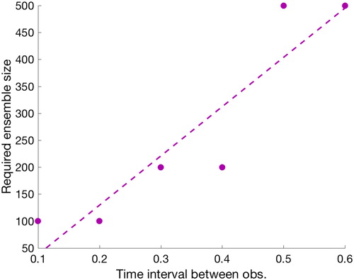
The PF-GR leads to the lowest RMSE for all setups we consider, but this comes at the cost of a large required ensemble size. The required ensemble size in fact increases with ΔT as shown in Fig. 5, where we plot the required ensemble size as a function of the time interval between observations. We define the required ensemble size as follows. For a given $N_{\mathrm{e}},$ we compute RMSE and compare this RMSE to the RMSE we computed with the PF-GR with $N_{\mathrm{e}}=1000.$ The required ensemble size is defined as the minimum ensemble size that leads to a difference in the RMSEs that is below a tolerance. Figure 5 thus illustrates what ensemble size the PF-GR requires to yield nearly the same RMSE as the PF-GR with $N_e=N_{e,\text{max}}=1,000.$ We note that with increasing nonlinearity, the required ensemble size increases and for strongly nonlinear problems a large ensemble size is required ($N_{\mathrm{e}}=500-1,000$). Note that this is independent of dimension. PFs require (exponentially) larger ensembles when the dimension increases to avoid collapse, but localization of PFs can prevent such extremely large ensembles. In the low-dimensional L63 problem, the large ensemble size is required because of the strong nonlinearity.

Fig. 5. Ensemble size of the PF-GR required to reach RMSE of the PF-GR with ensemble size $N_e=1,000$ as a function of the time interval between observations. The dots correspond to results we obtained by considering the ensemble sizes $N_{\mathrm{e}}=\{20,50,100,200,500,1000\},$ and the dashed line is a least squares fit.

In summary, we find that when the nonlinearity is weak ($\Delta T=0.1$), all DA methods considered here ‘work’ and lead to similar RMSE and spread (but at different costs and for different $N_{\mathrm{e}}$). In the regime of mild or medium nonlinearity ($0.1\le \Delta T\le 0.4$), the variational methods (varPS, varPS-nw and EDA) are characterized by an RMSE comparable to the PF-GR, but their computational cost is lower. In the regime of medium nonlinearity, the variational methods lead to smaller RMSE than the rank histogram filter (RHF) described by Anderson (2010) (see Fig. 8 of Metref et al., 2014 for the results), the EnKFs and the EnKS. For strong non-linearity, the variational methods lead to large RMSE, while the EnKF has modestly lower RMSE, and we describe the details of how this occurs below.

5.2.3. Discussion–mild and medium nonlinearity

Our main conclusion from Section 3 is that Gaussian approximations to posterior distributions are more appropriate than Gaussian approximations to the filtering prior when the problem is characterized by mild or medium nonlinearity ($0.1\le \Delta T\le 0.4$). The DA experiments with L63 provide numerical evidence that this is indeed the case. In particular, we note the smaller average skewness of the smoothing or filtering posterior distributions as compared to the filtering prior (see Fig. 4).

Small RMSE (and spread) of the PF-GR, which makes a Gaussian approximation of the filtering posterior distribution at each assimilation time, indicates that the the Gaussian approximation is reasonable. In other words, the filtering posterior distribution can be nearly Gaussian, even when the filtering prior is not nearly Gaussian. This can be illustrated further by considering the prior and posterior distributions of one DA cycle. Specifically, we perform one DA cycle, starting from a Gaussian prior distribution ${\mathbf{x}}_0\sim \mathcal{N}(\mu ,\mathbf{B}),$ where μ is a typical state of the L63 model and $\mathbf{B}$ is the climatological covariance (obtained by running a long simulation with L63 and computing the covariance). We then make an observation of all three state variables at $t=\Delta T$ with observation error covariance $\mathbf{R}=4{\mathbf{I}}_3$ and consider two intervals between observations, $\Delta T=0.1$ (mild nonlinearity) and $\Delta T=0.3$ (medium nonlinearity). We approximate the filtering prior and filtering/smoothing posterior distributions by the standard PF using a very large ensemble size. That is, we draw $N_{\mathrm{e}}={10}^6$ ensemble members, ${\mathbf{x}}_0^j,j=1,\dots ,N_{\mathrm{e}},$ from the Gaussian prior distribution and propagate each ensemble member to time $t=\Delta T$ to obtain the forecast ensemble ${\mathbf{x}}_{\Delta T}^j=\mathcal{M}({\mathbf{x}}_0^j).$ The forecast ensemble is distributed according to the filtering prior. We then compute weights $w^j\propto p(\mathbf{y}|{\mathbf{x}}_{\Delta T}^j)$ and resample the ensemble ${\mathbf{x}}_{\Delta T}^j$ with these weights. The resampled ensemble is distributed according to the filtering posterior $p_f({\mathbf{x}}_{\Delta T}|\mathbf{y}).$ We also resample the prior ensemble at time zero, ${\mathbf{x}}_0^j,$ with the same weights. This resampled ensemble is distributed according to the smoothing posterior $p_s({\mathbf{x}}_0|\mathbf{y}).$

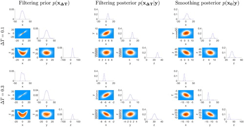
In Fig. 6, we plot histograms of the samples of the prior and posterior distributions in the form of ‘corner plots’ for two values of ΔT. A corner plot contains histograms of all one and two dimensional marginals of a multivariate distribution. The top row of Fig. 6 shows corner plots of the filtering prior (left), filtering posterior (center), and smoothing posterior (right) for a time interval between observations of $\Delta T=0.1$ (mild nonlinearity). The bottom rows show the same distributions for a larger time interval between observations of $\Delta T=0.3$ (medium nonlinearity). We see that the filtering prior evolves from being uni-modal for $\Delta T=0.1$ to multi-modal when $\Delta T=0.3.$ The observations, however, regularize the non-Gaussian filtering prior and lead to uni-modal posterior distributions (smoothing or filtering) for both values of ΔT. The posterior distributions (smoothing or filtering) are thus more amenable to Gaussian approximations than the filtering prior.

Fig. 6. Corner plots of prior and posterior distributions for two different time intervals between observations.

Variational algorithms (varPS, varPS-nw, EDA) yield a small RMSE, comparable to the PF-GR and smaller than RMSE of the EnKFs when the nonlinearity is mild or medium ($0.1\le \Delta T\le 0.4$). This too can be explained by posterior distributions being more amenable to Gaussian approximations than the filtering prior. Recall that the variational methods rely on Gaussian approximations of the smoothing prior and posterior and that the smoothing prior is in fact a posterior distribution (filtering posterior from the previous DA cycle). The EnKFs, however, make (indirect) use of a Gaussian approximation of the filtering prior. During an EnKF analysis only the mean and covariance of the filtering prior are computed; other, non-Gaussian, aspects of the filtering prior are subsequently ignored. The filtering prior, however, becomes more non-Gaussian when the time interval between observations increases. With larger time intervals between observations, non-Gaussian aspects of the filtering prior thus become more significant and, hence, the performance of the EnKF degrades. This explains, at least in part, why the EnKFs yields small RMSE when the time interval between the observations is short, but large RMSE when this time interval is long.

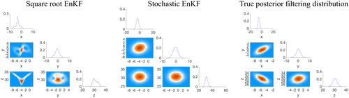
In addition, we recall that the square root EnKF operates slightly differently than the stochastic EnKF and in fact has a ‘more non-Gaussian’ analysis ensemble, see, e.g. Lawson and Hansen (2004). This is illustrated in Fig. 7, where we show corner plots of the filtering posterior distributions (analysis ensemble) of the square root EnKF ($N_{\mathrm{e}}={10}^4$) and of the stochastic EnKFs ($N_{\mathrm{e}}={10}^5$) for one cycle of the DA problem with $\Delta T=0.3.$ We note that the approximation of the filtering posterior distribution of the square root EnKF is ‘less Gaussian’ (bimodal) than the filtering posterior distribution of the stochastic EnKF. In view of the fact that the actual filtering posterior distribution (computed via the PF-GR with $N_{\mathrm{e}}={10}^6$) is well approximated by a Gaussian, it is not surprising that the stochastic EnKF yields smaller RMSE than the square root EnKF in this example where it has exaggerated the true amount of non-Gaussianity (see Hodyss and Campbell 2013 for further discussion).

Fig. 7. Corner plots of the analysis ensemble of of square root EnKF (left), stochastic EnKF (right). The time interval between observations is $\Delta T=0.3.$

Finally, we note that the results we obtain by the varPS and the varPS-nw are almost identical and the performance of both methods degrades at the same time interval between observations ($\Delta T=0.5,$ we investigate how this increase in RMSE occurs in more detail below). Recall that the varPS-nw samples a Gaussian approximation of the smoothing posterior and uses this Gaussian for inferences. The weights, used in the varPS, morph this Gaussian proposal distribution into a non-Gaussian smoothing posterior. Comparing the varPS and the varPS-nw reveals that the unweighted ensemble gives nearly identical results to the weighted ensemble, which implies that the varPS target distribution (smoothing posterior) is well approximated by the Gaussian proposal of the varPS. This, again, is numerical evidence that the smoothing posterior distribution is amenable to Gaussian approximations when the nonlinearity is mild to medium ($0.1\le \Delta T\le 0.5$). Similar results were obtained by other ensemble smoothers in other test problems with medium nonlinearity, see Sakov et al. (2012); Bocquet and Sakov (2013, 2014); Bocquet (2016); Evensen (2018).

We summarize the numerical evidence that Gaussian approximations of posterior distributions are more appropriate than Gaussian approximations of filtering prior distributions in the regime of mild to medium nonlinearity ($0.1\le \Delta T\le 0.4$).

1. Good performance of the PF-GR, which makes use of a Gaussian approximation of the filtering posterior distribution, suggests that the posterior distribution remains nearly Gaussian even when the nonlinearity is medium, leading to filtering priors that are not nearly Gaussian.

2. The fact that the RMSEs of the EnKFs, which make use of a Gaussian approximation of the filtering prior, are larger than the RMSEs of the variational methods, which make use of Gaussian approximations of posterior distributions, corroborates that posterior distributions are more amenable to Gaussian approximations than the filtering prior.

3. On average, the skewness is larger for the filtering prior than for the smoothing or filtering posterior distributions.

4. The fact that the stochastic EnKF, which yields a ‘more Gaussian’ analysis ensemble than the square root filter, leads to smaller RMSE than the square root filter suggests that the filtering posterior may indeed be well approximated by a Gaussian.

5. The fact that the weights in the varPS, which morph a Gaussian proposal into a non-Gaussian posterior distribution, have nearly no impact on RMSE suggests that the Gaussian proposal is a good approximation of a nearly Gaussian smoothing posterior.

The fact that the PF-GR (and other PFs) requires a larger ensemble size than the variational methods in the regime of medium nonlinearity may seem counterintuitive, but there is a simple explanation. We have seen above that in problems with medium nonlinearity, the smoothing posterior is nearly a Gaussian and that varPS and other variational methods explicitly exploit this structure. The PF-GR, however, does not make any assumptions of this kind during inference—the Gaussian approximation is only needed to initialize the next cycle. Thus, the PF-GR exploits less problem structure and, for that reason, is not as effective as the methods that do exploit near-Gaussian problem structure. When the problem really is nearly Gaussian one should make explicit use of it during DA; the fact that the PF-GR does not do this is thus a drawback of this method (when applied to problems with medium nonlinearity).

5.2.4. Discussion–strong nonlinearity

For long time intervals between observations, $\Delta T\ge 0.5,$ the filtering and smoothing distributions can be severely non-Gaussian and, during some DA cycles, multi-modal. One would expect that all methods we consider here should yield large errors, during a DA cycle in which the filtering and smoothing posterior distributions are multi-modal, because all methods, including the PF-GR, rely on Gaussian approximations of posterior distributions in one way or another. We found, however, that this is not always true: the Gaussian approximations may be inappropriate, but that does not necessarily lead to large RMSE.

An example of this situation is provided in Fig. 8 where we show corner plots of the filtering prior as well as the smoothing and filtering posterior distributions at cycle 631. The corner plots are obtained from the ensemble of the PF-GR with $N_{\mathrm{e}}={10}^5$ (top row of the figure). We note that all three distributions are multi-modal. We also show RMSE as a function of DA cycle and the varPS-nw approximations of the smoothing posterior and filtering posterior distributions ($N_{\mathrm{e}}=100,$ bottom row of the figure).

Fig. 8. Top: corner plots of filtering prior (left), filtering posterior (center) and smoothing posterior (right) for DA cycle 631 with $\Delta T=0.6.$ The histograms are obtained by running the PF-GR with $N_{\mathrm{e}}={10}^5.$ The red dots are the true states and the orange dots are the observations. Bottom: RMSE as a function of DA cycle (left) and the varPS-nw approximations of the filtering posterior (center) and smoothing posterior (right).

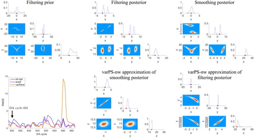
RMSEs of the PF-GR and the varPS-nw in Fig. 8 remain small at this cycle. Specifically, the varPS-nw approximates the multi-modal distribution by a uni-modal distribution centered at the dominant mode, which results in a small RMSE. Thus, while the Gaussian approximation used in the varPS-nw is clearly wrong, this deficiency cannot be diagnosed by considering RMSE. In fact, the multi-modal situation in Fig. 8 is virtually indistinguishable in terms of RMSE and spread to the uni-modal situation at DA cycle 632, illustrated in Fig. 9.

Fig. 9. Top: corner plots of filtering prior (left), filtering posterior (center) and smoothing posterior (right) for DA cycle 632 with $\Delta T=0.6.$ The histograms are obtained by running the PF-GR with $N_{\mathrm{e}}={10}^5.$ The red dots are the true states and the orange dots are the observations. Bottom: RMSE as a function of DA cycle (left) and the varPS-nw approximations of the filtering posterior (center) and smoothing posterior (right).

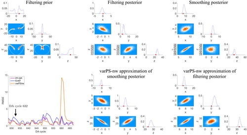
We note at cycle 632 that RMSE of the varPS-nw remains small because at the previous cycle (631) the varPS-nw has ‘picked’ the mode near the true state. Thus, the Gaussian approximation during cycle 631 does not to lead to large RMSE at cycle 632. Nonetheless, the Gaussian approximation is not valid because the other modes are ignored and there is no guarantee that the varPS will pick the correct mode (i.e. near the true state) at every cycle. Therefore, while RMSE is small, probabilistic inference made using the Gaussian approximation of the PDF will be unreliable. Moreover, the converse situation is also true. During several DA cycles, the optimization in the varPS-nw converges to a mode that is not near the true state and, for that reason, produces large RMSE (see also below for further explanation).

Similarly, the PF-GR has produced the distributions shown in Fig. 9 by making a Gaussian approximation to the multi-modal smoothing prior distribution shown in the center panel of the top row of Fig. 8. The RMSE of the PF-GR remains small at cycle 632, even though the Gaussian approximation made is clearly inappropriate. Therefore, the examples indicate that

1. under strong nonlinearity, Gaussian approximations to smoothing prior distributions may not be valid, but these Gaussian approximations may still lead to small RMSE in the average;

2. small RMSE is neither necessary nor sufficient to determine if a posterior distribution is uni-modal or if multiple modes are present;

3. small RMSE does not imply that the DA method accurately approximates the true posterior distribution.

These findings have ramifications on how one should test new DA methods for strongly nonlinear problems. Often, a simple model such as L63 or the Lorenz ’96 model (see Lorenz, 1996) are used to illustrate that a new DA method is ‘better’ than, say, the EnKF (see, e.g. Farchi and Bocquet, 2018). For such experiments to be useful, one should first investigate the degree to which the various distributions are non-Gaussian and if strong non-Gaussianity is indeed observed, performance indicators other than RMSE should be used if probabilistic inference is important.

Large RMSE can occur for a variational method when the scheme picks out ‘the wrong mode’ (the one not containing the true state). We wish to emphasize that there are other ways in which a large RMSE can occur in variational methods. We focus on the varPS-nw, but similar arguments can be made for the varPS or EDA. We have shown above that multi-modality of the smoothing posterior does not necessarily cause large RMSE in the varPS-nw if the optimization finds the ‘correct’ mode of the smoothing posterior distribution. In fact, the Gaussian approximation of the smoothing prior is not critical during many DA cycles, since the varPS-nw can produce RMSE comparable to the PF-GR (see left panel of bottom row of Figs. 8 and 9). We did however find situations with large RMSE in uni-modal situations when the minimization terminates unsuccessfully due to numerical issues. This situation is illustrated in Fig. 10. As before, we show corner plots of the filtering prior and filtering/smoothing posterior distributions (obtained by the PF-GR with $N_e={10}^6$) as well as the RMSE and the varPS-nw approximations of the posterior distributions. Focusing on the center panel in the bottom row, we can clearly identify that the optimization has returned a state that is not near the minimizer of the cost function or the true state. Such numerical issues cause the varPS-nw (and the other variational methods) to ‘lose track’ of the true state for a few cycles, before again yielding small RMSE (see left panel, bottom row of Fig. 10). The number of times such numerical issues occur during the 1200 DA cycles we consider in our experiments increases when the time interval between observations becomes longer. Numerical issues of this kind are not fixable by using weights (at finite ensemble size), as is indicated by the fact that the varPS and the varPS-nw lead to nearly identical RMSE.

Fig. 10. Top: corner plots of filtering prior (left), filtering posterior (center) and smoothing posterior (right) for DA cycle 660 with $\Delta T=0.6.$ The histograms are obtained by running the PF-GR with $N_{\mathrm{e}}={10}^5.$ The red dots are the true states and the orange dots are the observations. Bottom: RMSE as a function of DA cycle (left) and the varPS-nw approximations of the filtering posterior (center) and smoothing posterior (right).

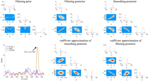
The numerical issues arise because the optimization is implemented in a simple manner. We use Matlab’s Gauss-Newton optimizer and compute the required gradient by finite differences (we did not bother with a tangent linear adjoint model because computations with L63 are inexpensive). We initialize the optimization with the prior mean and perform at most three Gauss-Newton iterations, or outer loops. Fewer than three outer loops are used when default tolerances are satisfied. We then use the result of the optimization without corrections if the optimizer has terminated unsuccessfully, i.e. if the computed mode is not a local minimum of the cost function. A more careful implementation of the optimization may help to reduce the RMSE of the variational methods to the RMSE levels of the PF-GR. In particular, one can consider tempering methods, as suggested by Evensen (2018), or re-start the optimizer with a new initial guess when optimization tolerances are not met. One can also envision running several optimizations to find several modes. We leave further investigation of more sophisticated optimization strategies for future work. Here, we report the conclusion that the optimization, routinely performed in variational methods, requires additional care when the problem is strongly nonlinear.

Finally, we notice that the EnKS yields smaller RMSE than the EnKF for short intervals between observations ($0.1\le \Delta T\le 0.2$). This suggests that the smoothing posterior distribution may be more amenable to Gaussian approximations than the filtering posterior distribution when the time interval between observations is small. This is further corroborated by the fact that the average skewness of the smoothing posterior distribution is smaller than the average skewness of the filtering posterior distribution when ΔT is small (see right panel of Fig. 4). However, for larger ΔT, this is not necessarily the case, as is illustrated in Fig. 11, where we show corner plots of the PF ensembles ($N_e={10}^6,$ as above) of the filtering prior and the filtering/smoothing posterior for a DA cycle with $\Delta T=0.5.$ The figure shows that the filtering prior and the smoothing posterior can be multi-modal while the filtering posterior is uni-modal (this is in agreement with the simple examples in Section 3.3). Thus, for this DA cycle, the filtering posterior is more amenable to Gaussian approximations than the smoothing posterior. The corner plot may appear at odds with the right panel of Fig. 4, which shows that the average (absolute) skewness of the posterior smoothing distribution is smaller than the average (absolute) skewness of the filtering posterior distribution. We must recall, however, that the skewness in Fig. 4 is averaged over the variables and over time. Thus, while on average the skewness may be smaller for the smoothing posterior than for the filtering posterior, this does not mean that this indicator of non-Gaussianity is always smaller or that the smoothing posterior is always more amenable to Gaussian approximations than the filtering posterior. In fact, we have already encountered a DA cycle in which both posterior distributions are multi-modal. At any given DA cycle of a strongly nonlinear problem, it is not possible for us to determine a priori which posterior distribution (smoothing or filtering) is more amenable to Gaussian approximation. In strongly nonlinear problems, this seems to in fact depend on the observation and DA cycle.

Fig. 11. Corner plots of the filtering prior, filtering posterior and smoothing posterior distributions for a long time interval between observations ($\Delta T=0.5,$ strong nonlinearity).

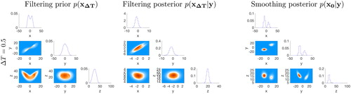
5.2.5. Other observation networks

We performed a series of further numerical experiments in which we changed the ‘observation network’ and considered smaller values for the observation error covariance $\mathbf{R},$ as well as observations of only a subset of the variables. We show some of our results in Fig. 12. In the left panel, we show results we obtain when all three variables are observed but the observation error covariance is smaller than above ($\mathbf{R}={\mathbf{I}}_3$). In the right panel, we show results obtained when we observe the x and z variable with small observation noise ($\mathbf{R}=0.1 {\mathbf{I}}_2$). All scenarios we considered exhibit the same qualitative trends: the PF-GR gives consistently the smallest RMSE, but in the regime of medium nonlinearity, the variational methods lead to errors as small as the PF-GR and smaller than for the EnKF. This suggests that these trends are not tied to one specific set up of a L63 problem but may indeed be indicative of what to expect for a class of nonlinear DA problems.

Fig. 12. RMSE as a function of the time interval between observations for a fully observed L63 system (left) and a partially observed L63 system (right).

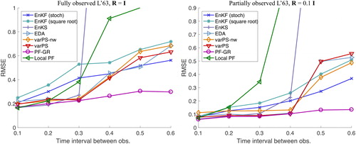
5.3. Higher-dimensional example: KdV

The L63 model has three dimensions and, for that reason, localization is not required for this example. Higher dimensional models, however, require that the algorithms be localized. Localization of ensemble covariances in variational methods, the EnKF and the EnKS is well understood and has been used in practice for many years. Localization of PFs, however, is not yet as well understood and one can expect that localization schemes introduce additional errors. The numerical experiments with L63 suggest that errors due to Gaussian approximations of posterior distributions are not critical in the regime of medium nonlinearity. A natural question is: are errors due to Gaussian approximations of posterior distributions perhaps less severe than errors introduced by localization of the PF.

We use the variable-coefficient, KdV equation of Hodyss and Nathan (2006, 2007) as a test problem, viz. (20) $$\frac{\partial A}{\partial t}-\frac{{\partial }^{3}A}{\partial x^3}+m_p\left(x\right)\frac{\partial A}{\partial x}+m_g\left(x\right)A-A\frac{\partial A}{\partial x}=0$$(20) where (21) $$m_p\left(x\right)=1-e^{-a{x}^2},\hspace{1em}{m}_g\left(x\right)=-2ax{e}^{-a{x}^2},\hspace{1em}a=0.0005,$$(21) on the domain $x\in [-25\pi ,25\pi ].$ This equation is a simple model of nonlinear waves in variable media. Hodyss and Nathan (2006, 2007) have shown that there exist two classes of instabilities owing to the spatially varying coefficients that correspond to oscillatory wave packets and smooth envelope structures. These instabilities grow to finite amplitude, invoke wave breaking, and subsequently spawn new solitary waves and other nonlinear waves. An example solution to (20) is presented in Fig. 13.

Fig. 13. An example solution plotted in space and through time for the variable-coefficient KdV equation. The solitary waves are bouncing back-and-forth within a “potential well’ whose width is approximately defined between –40 and 40.

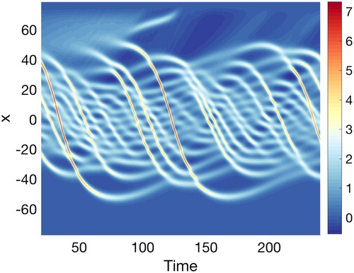
5.3.1. Setup, tuning and diagnostics

We consider a discretization of the equation on a regular grid, leading to a state vector of dimension $N_{\mathrm{x}}=128$ and use a pseudo-spectral method combined with a third order RK in time (time step $\Delta t=0.1$). The observations are also taken on a regular grid and we observe every other grid point ($N_{\mathrm{y}}=64$ observations). The observation error covariance is chosen to be a diagonal matrix whose diagonal elements are 10% of the true state at observation time. We consider cases where observations are available every ΔT time units and we vary ΔT. As before in the L63 example, larger ΔT makes the filtering prior ‘more non-Gaussian’ due to the nonlinear dynamics. This does not mean, however, that the posterior distributions are also strongly non-Gaussian. We perform synthetic data experiments of 1,200 DA cycles and compute RMSE and spread for all DA algorithms we consider (stochastic and square root EnKF, EnKS, varPS-new, PF-GR, PF-PR-GR, local PF). The first 200 cycles are discarded as spin up. All algorithms start with an ensemble of a spun up EnKF.

We tuned the localization and inflation parameters on shorter DA experiments with 120 DA cycles, discarding the first 20 cycles as spin up. The inflation is ‘prior inflation’ as described in the context of L63 (see Section 5.2.1). The localization of the EnKF and the EnKS is based on a circulant localization matrix that is defined from Fourier basis functions. Briefly, we define a matrix, E, whose columns are the sine and cosine functions properly normalized and arranged from smallest to largest wavenumber such that $\mathbf{E}{\mathbf{E}}^T=\mathbf{I}.$ We make use of the property that the Fourier transform of a Gaussian is another Gaussian and, subsequently, define a diagonal matrix, Γ, whose diagonal is a Gaussian as a function of wavenumber and for which the length-scale parameter may be shown to be related to the correlation length-scale inherent to the resulting localization matrix, ${\mathbf{C}}_L=\mathbf{E}\Gamma {\mathbf{E}}^T.$ We then tune the length scale parameter. We believe that the precise choice of the localization matrix is not critical to our results. The use of other schemes, e.g. Gaspari-Cohn, can be expected to produce similar results. To tune the localization of PF-PR-GR (see Section 2.3.2) we consider neighborhoods containing 1–5 grid points to the left and right.

We considered several ensemble sizes, but below only show results for $N_{\mathrm{e}}=200$ for the EnKFs, the EnKS, the PF-PR-GR, the local PF and the varPS-nw and for $N_{\mathrm{e}}={10}^4$ for the PF-GR. The large ensemble size is necessary for the PF-GR because the filter is not localized. Note that we are not suggesting that the PF-GR is a viable DA method in practice; the main purpose of the PF-GR is simply to serve as a benchmark solution for this problem.

5.3.2. Results

We plot RMSE as a function of the time interval between observations in Fig. 14. We also computed the spread for each DA method and found that spread and RMSE are comparable. As we tuned RMSE and spread to match we do not plot spread for clarity.

Fig. 14. RMSE as a function of the time interval between observations for a partially observed KdV system.

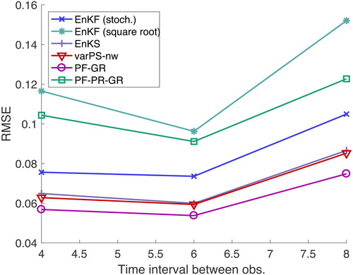
The results are qualitatively the same as for the low-dimensional L63 example: we find that the PF-GR gives consistently the smallest RMSE, but also requires the largest ensemble size. The smoothing algorithms (varPS-nw and EnKS) come close to the performance of the the PF-GR, which suggests that the smoothing posterior in this example is nearly Gaussian. The reason is that we consider a case with many observations and small observation error variance; hence, the regularization of the filtering prior by the observations is strong and posterior distributions are nearly Gaussian. As in L63, we also find that the stochastic EnKF performs slightly better than the square root filter (and for the same reasons). We made an effort to thoroughly tune the local PF; however, we could not find a configuration in which the local PF gives RMSE comparable to the RMSE of the other algorithms. This could be due to insufficient tuning, or could be interpreted as another hint at the fact that the inflation of our implementation of the local PF is problematic, especially when the observation noise is small. Such issues are addressed in Poterjoy et al. (2018). More generally, our results with the local PF can be viewed as a piece of evidence that inflation, or jittering, of PFs is as important as localization—we had no luck with PFs without inflation in low-dimensional problems and the inflation proves problematic in this higher-dimensional example as well.

In contrast to the L63 tests, the KdV tests require localization of PFs to avoid extremely large ensemble sizes. This allows us to study the additional error due to localization and how these errors compare with errors due to Gaussian approximation. We note that the RMSE of the PF-PR-GR with $N_{\mathrm{e}}=200$ is larger than the RMSEs of the PF-GR with $N_{\mathrm{e}}={10}^4,$ the varPS-nw ($N_{\mathrm{e}}=200$), the EnKS ($N_{\mathrm{e}}=200$), and the stochastic EnKF ($N_{\mathrm{e}}=200$). The RMSE of the PF-PR-GR ($N_{\mathrm{e}}=200$), however, is smaller than what we can obtain by the square root EnKF ($N_{\mathrm{e}}=200$). This suggests that localization of the PF is not necessarily a remedy for all issues with PFs and their collapse: unless the localization is done carefully, it may introduce additional errors that are more severe than errors one causes by Gaussian approximations of posterior distributions in variational methods such as EDA or varPS/varPS-nw. As indicated above, our localization scheme may not be optimal, yet the experiments with the KdV equation suggest that a LETKF-style localization of the PF may not be viable, at least in some nonlinear problems. This is also compatible with the results reported in Potthast et al. (2018) and Farchi and Bocquet (2018), where a similarly localized PF is applied to an operational NWP system and yields results that are slightly worse (in terms of RMSE) than what one can obtain by an EnKF.

6. Summary and discussion

We have presented mathematical arguments and numerical evidence that suggest that posterior distributions can be nearly Gaussian even when the numerical model is nonlinear, resulting in filtering prior distributions that are not nearly Gaussian. The findings of this paper further suggest several ramifications for DA in NWP. We summarize our main conclusions.

1. When nonlinearity is mild, the various distributions in filters and smoothers are nearly Gaussian and the various DA methods (EnKF, EnKS, PF, PS and variational methods) lead to similar RMSE and spreads, but at different costs. Methods that make use of near-Gaussian problem structure (EnKF, EnKS, variational methods) tend to be more effective than methods that do not exploit this structure, e.g. the PF.

2. When nonlinearity is medium, DA algorithms that make use of Gaussian approximations of posterior distributions, e.g. variational methods and variational PS, can be more appropriate than the EnKF, which makes use of Gaussian approximations of the filtering prior. Variational methods are also more appropriate than PFs because PFs do not exploit near-Gaussian problem structure and, for that reason, require larger ensembles.

3. In high-dimensional problems with medium nonlinearity, localization of the PF must be done carefully, or else additional errors due to localization can be larger than errors due to Gaussian approximations of posterior distributions.

4. PFs are worthwhile if a DA problem is strongly nonlinear, with severely non-Gaussian posterior distributions; in this regime, however, larger ensemble sizes than usually considered are required (hundreds to thousands, see also Poterjoy et al., 2018).

5. Variational methods are sensitive to the numerical implementation of the optimization in strongly nonlinear problems and can produce large errors unless the optimization is implemented carefully. The EnKF may be a useful alternative as the EnKF does not require numerical optimization and can lead to similar RMSE as variational methods with its ‘simple’ optimization strategy in strongly nonlinear problems. Probabilistic inferences based on the EnKF, however, are likely to be poor in strongly nonlinear problems with multi-modal distributions.

The main motivation for using PFs is to be able to capture non-Gaussian aspects of the (filtering) posterior distribution. For that reason, PFs make no assumptions about underlying problem structure. Localized PFs rely on the assumption that the model is ‘local’, i.e. that interactions of state variables are constrained to neighborhoods and that observations have a local, not global effect. It follows that PFs, even optimal ones, optimally localized, cannot ‘beat’ the EnKF in linear problems because a localized EnKF exploits linearity of the model and local problem structure (see also Morzfeld et al., 2018). This fact, in conjunction with our comparisons of the PF with variational methods and PS in problems with mild and medium nonlinearity indicate that PFs are worthwhile only if the nonlinearity is strong (multi-modal posterior distribution).

Strong nonlinearity and severely non-Gaussian posterior distributions, however, require a re-thinking of the overall DA approach. For example state estimates are typically based on posterior means or modes (or approximations thereof), but posterior means or modes are not adequate as state estimates in multi-modal situations. It is unclear to us how to produce a single state estimate if one detects two (or more) modes in the filtering posterior. In addition, DA algorithms are often evaluated based on RMSE and spread. When the posterior distributions are non-Gaussian (multi-modal), then these two quantities may no longer be sufficient to adequately assess the performance of a numerical DA method.

The ensemble size of the PF in a strongly nonlinear problem should be expected to be large (see also the conclusions of Poterjoy et al., 2018). The reason is that even scalar distributions, with large skew or multiple modes, are not easily represented by small ensembles. Our experiments with L63 suggest that ensembles sizes of several hundred or even thousands should be considered when dealing with severely non-Gaussian problems (and otherwise PFs should be avoided as explained above). Such large ensembles are computationally challenging to produce with operational NWP codes. Perhaps one way forward could be to pursue a ‘hybrid’ or multi-scale approach, where the bulk of the state is estimated by a suitable nearly Gaussian technique (variational DA or PS), and where PFs and non-Gaussian methods are only used on a subset of the state, see also Robert and Künsch (2017). This, however, requires a deep understanding of the nonlinearity and non-Gaussianity of the NWP DA problem, which at this point, is missing.

The most pressing question for NWP is: how nonlinear is a NWP problem and how does this nonlinearity change, e.g. when the resolution of the model is refined or when the observation network is changed. It is often said that the ‘problem is more nonlinear when the resolution is increased’ (see, e.g. Farchi and Bocquet, 2018), but it is unclear what this statement means in regards to ‘how non-Gaussian’ the resulting posterior distributions are, in particular if the observation network is also changed. Our work does not give answers to these important questions, but we have worked out guidelines that suggest which DA algorithms are suitable depending on the type of non-Gaussianity of posterior and prior distributions one encounters in NWP.

Supplementary data

Supplemental data for this article can be accessed https://10.1080/16000870.2019.1600344.

Disclosure statement

No potential conflict of interest was reported by the authors.

Additional information

Funding

MM was supported by the Office of Naval ResearchN00173- 17-2-C003 [grant number N00173-17-2-C003]; by an Alfred P. Sloan Research Fellowship, and by the National Science Foundation [grant number DMS-1619630]. DH gratefully acknowledges support from the Office of Naval Research [PE-0601153N].

Appendix: Covariance matrices of smoothing prior and posterior are smaller than the covariance matrix of the filtering prior and posterior

In Section 3.1, it was stated that the smoothing posterior has smaller variance than the filtering posterior and that the smoothing prior has smaller variance than the filtering posterior. We can make these statements mathematically precise under additional simplifying assumptions. First, we require that the model be linear, i.e. (22) $${\mathbf{x}}_n=\mathbf{M}{\mathbf{x}}_{n-1},$$(22) and that the largest singular value of the model matrix $\mathbf{M},$ is larger than one. Recall that the largest singular value of a matrix is the induced two-norm. Generically, we write the largest singular value of a matrix $\mathbf{A}$ as $\left|\right|\mathbf{A}|{|}_2={\widehat{\sigma }}_{\mathbf{A}}.$ Let ${\mu }_{n-1}$ and ${\mathbf{P}}_{n-1}$ be the mean and covariance of the filtering posterior at time n – 1. Then the smoothing and filtering prior at cycle n are (23) $$p\left({\mathbf{x}}_{1:n-1}\right|{\mathbf{y}}_{1:n-1})=\mathcal{N}({\mu }_{n-1},{\mathbf{P}}_{n-1}),$$(23) (24) $$p\left({\mathbf{x}}_{1:n}\right|{\mathbf{y}}_{1:n-1})=\mathcal{N}(\mathbf{M}{\mu }_{n-1},{\mathbf{P}}^f),$$(24) where the forecast covariance ${\mathbf{P}}^f=\mathbf{M}{\mathbf{P}}_{n-1}{\mathbf{M}}^T.$ We further assume that the covariance matrix ${\mathbf{P}}_{n-1}$ and the model matrix can be decomposed as (25) $${\mathbf{P}}_{n-1}=\mathbf{U}\Gamma {\mathbf{U}}^T,\hspace{1em}\mathbf{M}=\mathbf{V}\Lambda {\mathbf{U}}^T,$$(25) where Γ and Λ are diagonal matrices and where $\mathbf{U}$ and $\mathbf{V}$ are orthogonal matrices, i.e. $\mathbf{V}{\mathbf{V}}^T={\mathbf{I}}_{N_{\mathrm{x}}},\mathbf{U}{\mathbf{U}}^T={\mathbf{I}}_{N_{\mathrm{x}}}.$ In other words, the eigenvectors of the covariance matrix are equal to the right singular vectors of the model matrix. This assumption is consistent with typical example problems, e.g. Lorenz (1996), where the covariance and model matrices are both homogeneous and circulant (Toeplitz). Under our assumptions: (26) $$\left|\right|{\mathbf{P}}^f|{|}_2=|\left|\mathbf{M}{\mathbf{P}}_{n-1}{\mathbf{M}}^T\right|{|}_2=\left|\right|\mathbf{V}\Lambda \Gamma \Lambda {\mathbf{V}}^T|{|}_2=||\Lambda \Gamma \Lambda |{|}_2={\widehat{\sigma }}_{\mathbf{M}}^2{\widehat{\sigma }}_{{\mathbf{P}}_{n-1}}>{\widehat{\sigma }}_{{\mathbf{P}}_{n-1}}=\left|\right|{\mathbf{P}}_{n-1}|{|}_2.$$(26)

Thus, the covariance of the smoothing prior is less than the covariance of the filtering prior (in the induced two-norm).

Using the same notation as above, and denoting the mean and covariance of the smoothing posterior by μ^s and ${\mathbf{P}}^s,$ we have (27) $$p_s\left({\mathbf{x}}_{1:n-1}\right|{\mathbf{y}}_{1:n})=\mathcal{N}({\mu }_{n-1}^s,{\mathbf{P}}_{n-1}^s),$$(27) (28) $$p_f\left({\mathbf{x}}_{1:n}\right|{\mathbf{y}}_{1:n})=\mathcal{N}({\mu }_n,{\mathbf{P}}_n),$$(28) where ${\mathbf{P}}_n=\mathbf{M}{\mathbf{P}}_{n-1}^s{\mathbf{M}}^T.$ Assuming that ${\mathbf{P}}_{n-1}^s=\mathbf{U}\Phi {\mathbf{U}}^T,$ where $\mathbf{U}$ is as above and $\Phi$ is a diagonal matrix, the same arguments as above give: (29) $$\left|\right|{\mathbf{P}}_{n-1}^s|{|}_2<|\left|{\mathbf{P}}_n\right|{|}_2.$$(29)

Thus, the smoothing posterior has a smaller covariance than the filtering posterior at the same cycle.

References

- Anderson, J. L. 2010. A non-gaussian ensemble filter update for data assimilation. Mon. Wea. Rev. 138, 4186–4198. doi:10.1175/2010MWR3253.1
- Bardsley, J., Solonen, A., Haario, H. and Laine, M. 2014. Randomize-then-optimize: A method for sampling from posterior distributions in nonlinear inverse problems. SIAM J. Sci. Comput. 36, A1895–A1910. doi:10.1137/140964023
- Bengtsson, T., Bickel, P. and Li, B. 2008. Curse of dimensionality revisited: the collapse of importance sampling in very large scale systems. IMS Collect. 2, 316–334.
- Bickel, P., Bengtsson, T. and Anderson, J. 2008. Sharp failure rates for the bootstrap particle filter in high dimensions. IMS Collect. 3, 318–329.
- Bocquet, M. 2011. Ensemble Kalman filtering without the intrinsic need for inflation. Nonlin. Process. Geophys. 18, 735–750. doi:10.5194/npg-18-735-2011
- Bocquet, M. 2016. Localization and the iterative ensemble Kalman smoother. Q. J. Roy. Meteorol. Soc. 142, 1075–1089. doi:10.1002/qj.2711
- Bocquet, M. and Sakov, P. 2013. Joint state and parameter estimation with an iterative ensemble kalman smoother. Nonlin. Process. Geophys. 20, 803–818. doi:10.5194/npg-20-803-2013
- Bocquet, M. and Sakov, P. 2014. An iterative ensemble Kalman smoother. Q. J. Roy. Meteorol. Soc. 140, 1521–1535. doi:10.1002/qj.2236
- Bonavita, M., Isaksen, L. and Hólm, E. 2012. On the use of EDA background-error variances in the ECMWF 4D-Var. Q. J. Roy. Meteorol. Soc. 138, 1540–1559. doi:10.1002/qj.1899
- Buehner, M. 2005. Ensemble-derived stationary and flow-dependent background-error covariances: Evaluation in a quasi-operational NWP setting. Q. J. Roy. Meteorol. Soc. 131, 1013–1043. doi:10.1256/qj.04.15
- Doucet, A., de Freitas, N. and Gordon, N., eds. 2001. Sequential Monte Carlo Methods in Practice. Springer, New York.
- Evensen, G. 2006. Data Assimilation: The Ensemble Kalman Filter. Springer, Berlin Heidelberg.
- Evensen, G. 2018. Analysis of iterative ensemble smoothers for solving inverse problems. Comput. Geosci. 22, 885–908. doi:10.1007/s10596-018-9731-y
- Farchi, A., and Bocquet, M. 2018. Review article: Comparison of local particle filters and new implementations. Nonlinear Process. Geophys. Discuss. 1–63. doi:10.5194/npg-2018-15
- Hamill, T. M., Whitaker, J. and Snyder, C. 2001. Distance-dependent filtering of background covariance estimates in an ensemble Kalman filter. Mon. Wea. Rev. 129, 2776–2790. doi:10.1175/1520-0493(2001)129<2776:DDFOBE>2.0.CO;2
- Hodyss, D. and Campbell, W. 2013. Square root and perturbed observation ensemble generation techniques in kalman and quadratic ensemble filtering algorithms. Mon. Wea. Rev. 141, 2561–2573. doi:10.1175/MWR-D-12-00117.1
- Hodyss, D. and Nathan, T. 2007. The role of forcing in the local stability of stationary long waves. Part 1. Linear dynamics. J. Fluid Mech. 576, 349–376. doi:10.1017/S0022112006004307
- Hodyss, D. and Nathan, T. R. 2006. Instability of variable media to long waves with odd dispersion relations. Commun. Math. Sci. 4, 669–676. doi:10.4310/CMS.2006.v4.n3.a10
- Hodyss, D., Campbell, W. F. and Whitaker, J. S. 2016. Observation-dependent posterior inflation for the ensemble kalman filter. Mon. Wea. Rev. 144, 2667–2684. doi:10.1175/MWR-D-15-0329.1
- Houtekamer, P. and Mitchell, H. 2001. A sequential ensemble Kalman filter for atmospheric data assimilation. Mon. Wea. Rev. 129, 123–136. doi:10.1175/1520-0493(2001)129<0123:ASEKFF>2.0.CO;2
- Hunt, B. R., Kostelich, E. J. and Szunyogh, I. 2007. Efficient data assimilation for spatiotemporal chaos: A local ensemble transform kalman filter. Phys. D 230, 112–126. doi:10.1016/j.physd.2006.11.008
- Kuhl, D., Rosmond, T., Bishop, C., McLay, J. and Baker, N. 2013. Comparison of hybrid ensemble/4DVar and 4DVar within the NAVDAS-AR data assimilation framework. Mon. Wea. Rev. 141, 2740–2758. doi:10.1175/MWR-D-12-00182.1
- Lawson, W. and Hansen, J. 2004. Implications of stochastic and deterministic filters as ensemble-based data assimilation methods in varying regimes of error growth. Mon. Wea. Rev. 136, 1966–1981.
- Lee, Y. and Majda, A. 2016. State estimation and prediction using clustered particle filters. Proc. Natl. Acad. Sci. USA. 113, 14609–14614. doi:10.1073/pnas.1617398113
- Lei, J. and Bickel, P. 2011. A moment matching ensemble filter for nonlinear non-Gaussian data assimilation. Mon. Wea. Rev. 139, 3964–3973. doi:10.1175/2011MWR3553.1
- Liu, C., Xiao, Q. and Wang, B. 2008. An ensemble-based four-dimensional variational data assimilation scheme. Part I: Technical formulation and preliminary test. Mon. Wea. Rev. 136, 3363–3373. doi:10.1175/2008MWR2312.1
- Lorenc, A., Bowler, N., Clayton, A., Pring, S. and Fairbairn, D. 2015. Comparison of hybrid-4DEnVar and hybrid-4DVar data assimilation methods for global NWP. Mon. Wea. Rev. 143, 212–229. doi:10.1175/MWR-D-14-00195.1
- Lorenz, E. 1963. Deterministic nonperiodic flow. J. Atmos. Sci. 20, 130–141. doi:10.1175/1520-0469(1963)020<0130:DNF>2.0.CO;2
- Lorenz, E. N. 1996. Predictability: A problem partly solved, Vol. 1. In: Proceedings of the ECMWF Seminar on predictability, Reading, United Kingdom, 1–18.
- Mandel, J., Cobb, L. and Beezley, J. 2011. On the convergence of the ensemble Kalman filter. Appl. Math. (Prague) 56, 533–541. doi:10.1007/s10492-011-0031-2
- Metref, S., Cosme, E., Snyder, C. and Brasseur, P. 2014. A non-gaussian analysis scheme using rank histograms for ensemble data assimilation. Nonlin. Process. Geophys. 21, 869–885. doi:10.5194/npg-21-869-2014
- Morzfeld, M., Hodyss, D. and Poterjoy, J. 2018. Variational particle smoothers and their localization. Q. J. Roy. Meteor. Soc. 144, 806–825. doi:10.1002/qj.3256
- Morzfeld, M., Hodyss, D. and Snyder, C. 2017. What the collapse of the ensemble Kalman filter tells us about particle filters. Tellus A 69, 1283809. doi:10.1080/16000870.2017.1283809
- Penny, S. and Miyoshi, T. 2015. A local particle filter for high dimensional geophysical systems. Nonlinear Process. Geophys. 2, 1631–1658. doi:10.5194/npgd-2-1631-2015
- Posselt, D., Hodyss, D. and Bishop, C. 2014. Errors in ensemble Kalman smoother estimates of cloud microphysical parameters. Mon. Wea. Rev. 142, 1631–1654. doi:10.1175/MWR-D-13-00290.1
- Poterjoy, J. 2016. A localized particle filter for high-dimensional nonlinear systems. Mon. Wea. Rev. 144, 59–76. doi:10.1175/MWR-D-15-0163.1
- Poterjoy, J. and Anderson, J. 2016. Efficient assimilation of simulated observations in a high-dimensional geophysical system using a localized particle filter. Mon. Wea. Rev. 144, 2007–2020. doi:10.1175/MWR-D-15-0322.1
- Poterjoy, J. and Zhang, F. 2015. Systematic comparison of four-dimensional data assimilation methods with and without the tangent linear model using hybrid background error covariance: E4DVar versus 4DEnVar. Mon. Wea. Rev. 143, 1601–1621. doi:10.1175/MWR-D-14-00224.1
- Poterjoy, J., Sobash, R. and Anderson, J. 2017. Convective-scale data assimilation for the weather research and forecasting model using the local particle filter. Mon. Wea. Rev. 145, 1897–1918. doi:10.1175/MWR-D-16-0298.1
- Poterjoy, J., Wicker, L. and Buehner, M. 2018. Progress toward the application of a localized particle filter for numerical weather prediction. Mon. Wea. Rev.
- Potthast, R., Walter, A. and Rhodin, A. 2018. A localised adaptive particle filter within an operational NWP framework. Mon. Wea. Rev.
- Reich, S. 2013. A nonparametric ensemble transform method for Bayesian inference. Mon. Wea. Rev. 35, 1337–1367.
- Robert, S. and Künsch, H. R. 2017. Localizing the ensemble Kalman particle filter. Tellus A 69, 1282016. doi:10.1080/16000870.2017.1282016
- Sakov, P., Oliver, D. S. and Bertino, L. 2012. An iterative EnKF for strongly nonlinear systems. Mon. Wea. Rev. 140, 1988–2004. doi:10.1175/MWR-D-11-00176.1
- Snyder, C. 2011. Particle filters, the “optimal” proposal and high-dimensional systems. Proceedings of the ECMWF Seminar on Data Assimilation for Atmosphere and Ocean, Reading, UK, 1–10.
- Snyder, C., Bengtsson, T., Bickel, P. and Anderson, J. 2008. Obstacles to high-dimensional particle filtering. Mon. Wea. Rev. 136, 4629–4640. doi:10.1175/2008MWR2529.1
- Snyder, C., Bengtsson, T. and Morzfeld, M. 2015. Performance bounds for particle filters using the optimal proposal. Mon. Wea. Rev. 143, 4750–4761. doi:10.1175/MWR-D-15-0144.1
- Talagrand, O. and Courtier, P. 1987. Variational assimilation of meteorological observations with the adjoint vorticity equation. I: Theory. Q. J. Roy. Meteor. Soc. 113, 1311–1328. doi:10.1002/qj.49711347812
- Tippet, M., Anderson, J., Bishop, C., Hamill, T. and Whitaker, J. 2003. Ensemble square root filters. Mon. Wea. Rev. 131, 1485–1490. doi:10.1175/1520-0493(2003)131<1485:ESRF>2.0.CO;2
- Tödter, J. and Ahrens, B. 2015. A second-order exact ensemble square root filter for nonlinear data assimilation. Mon. Wea. Rev. 143, 1337–1367.
- Weir, B., Miller, R. N. and Spitz, Y. H. 2013. A potential implicit particle method for high-dimensional systems. Nonlin. Process. Geophys. 20, 1047–1060. doi:10.5194/npg-20-1047-2013