On the consistency of the local ensemble square root Kalman filter perturbation update

Abstract

We examine the perturbation update step of the ensemble Kalman filters which rely on covariance localisation, and hence have the ability to assimilate non-local observations in geophysical models. We show that the updated perturbations of these ensemble filters are not to be identified with the main empirical orthogonal functions of the analysis covariance matrix, in contrast with the updated perturbations of the local ensemble transform Kalman filter (LETKF). Building on that evidence, we propose a new scheme to update the perturbations of a local ensemble square root Kalman filter (LEnSRF) with the goal to minimise the discrepancy between the analysis covariances and the sample covariances regularised by covariance localisation. The scheme has the potential to be more consistent and to generate updated members closer to the model’s attractor (showing fewer imbalances). We show how to solve the corresponding optimisation problem and discuss its numerical complexity. The qualitative properties of the perturbations generated from this new scheme are illustrated using a simple one-dimensional covariance model. Moreover, we demonstrate on the discrete Lorenz–96 and continuous Kuramoto–Sivashinsky one-dimensional low-order models that the new scheme requires significantly less, and possibly none, multiplicative inflation needed to counteract imbalance, compared to the LETKF and the LEnSRF without the new scheme. Finally, we notice a gain in accuracy of the new LEnSRF as measured by the analysis and forecast root mean square errors, despite using well-tuned configurations where such gain is very difficult to obtain.

Keywords:

• data assimilation
• ensemble Kalman filter
• ensemble square root Kalman filter
• covariance localisation
• perturbation ensemble update

1. Context

The ensemble Kalman filter (EnKF) has been shown to be a successful data assimilation technique for filtering and forecasting in complex chaotic fluids (see Evensen, 2009, and references therein). Thus, it has been used as a powerful tool for deterministic as well as ensemble forecast of geofluids (Houtekamer et al., 2005; Sakov et al., 2012). It is based on an unavoidably limited ensemble size due to the numerical cost of realistic geofluid models. As a trade-off, the noisy covariance estimates obtained from this ensemble must be regularised, primarily using the technique known as localisation. Localisation was shown to be necessary with a chaotic model whenever the ensemble size is smaller than the number of unstable and neutral modes of the dynamics (Bocquet and Carrassi, 2017) and possibly still beneficial for larger ensemble size (Anderson, 2012).

Localisation assumes that correlations between spatially distant parts of the physical system decrease at a fast rate with the physical distance, e.g. exponentially. As a consequence, one can make the assimilation of observations local or, alternatively, artificially taper distant spurious correlations that emerge from sampling errors (Hamill et al., 2001; Houtekamer and Mitchell, 2001). As a result, two broad types of localisation techniques have been considered so far: domain localisation and covariance localisation.

Domain localisation consists of a collection of local updates, e.g. centred on the grid points using nearby observations (Houtekamer and Mitchell, 2001; Ott et al., 2004). These updates can be carried out in parallel since they are assumed independent. The full updated ensemble is obtained by assembling these local updates. Moreover, the transition between the updates of two adjacent domains can be made smoother by tapering the precision of the attached observations, which leads to refined domain localisation approaches (Hunt et al., 2007; Nerger and Gregg, 2007). This can reduce the imbalance generated by assembling this collection of updates to form the global updated ensemble (Kepert, 2009; Greybush et al., 2011). Imbalance is defined in this study as a measure of the distance between the updated ensemble members and the model’s attractor, a discrepancy one would like to be as small as possible.

The second type of localisation is covariance localisation which is enforced through a direct tapering of all sample covariances. This is usually implemented using a Schur product of the sample covariance matrix with a correlation matrix with fast decreasing entries with the distance. The Schur product output is mathematically guaranteed to be a covariance matrix and, with a proper localisation correlation matrix, is likely to make the regularised covariance matrix full-rank.

Even though based on the same diagnostic, the two types of localisation are distinct in their philosophy, and in their algorithmic and numerical implementation. Domain localisation does not allow assimilating non-local observations such as radiances without ad hoc approximations, but the scheme is embarrassingly parallel by nature. Covariance localisation is mathematically grounded in the tapering of the background covariance only and could hence be seen as a well understood scheme, but its numerical implementation, relying on a single global analysis, is much less simple, especially for deterministic EnKFs. In practice, the two schemes have been shown to coincide in the limit where the analysis is driven by the background statistics, i.e. weak assimilation (Sakov and Bertino, 2011). They could differ otherwise.

Note that a third route for localisation is through the statistics technique known as shrinkage. It consists in adding a possibly adaptively tuned full-rank covariance matrix to the background error covariance matrix (see Hannart and Naveau, 2014, and references therein). The approach was successfully tested by Bocquet et al. (2015) in the case of a hybrid EnKF.

From a theoretical standpoint, the localisation schemes seem ad hoc in spite of their remarkable practical efficiency. There could be room for improvements based on theoretical considerations. For instance, localisation can be made multiscale (Buehner and Shlyaeva, 2015) or adaptive (Anderson and Lei, 2013; Ménétrier et al., 2015; De La Chevrotière and Harlim, 2017). However, these two subjects are not topics of this paper.

In this paper, we would like to revisit the perturbation update step of the EnKF when relying on covariance localisation. We especially focus on the local ensemble square root Kalman filter (LEnSRF). Traditional EnKF schemes offer a consistent view on the perturbations which are generated in the analysis and propagated in the forecast. By consistent, it is meant here that the sample statistics (mean and covariances) of the analysed and forecast ensembles are supposed to match those of the actual analysis and forecast distributions. This consistency in the EnKFs is often approximate as evidenced by the need for inflation. Our goal is to further improve on this consistency and offer a more coherent view on the perturbations in the EnKF.

In Section 2, we recall the principle of covariance localisation, explain and shed some new light on how the perturbations are updated. In Section 3, we discuss the consistency of the perturbation update, and we propose a new approach for this update. In addition, we discuss the numerical cost of this approach. In Section 4, we present numerical results on a simple covariance model as well as on two low-order chaotic models that show potential benefits of the new scheme. Conclusions are given in Section 5.

2. Motivation

2.1. Principle of covariance localisation

In this study, the main focus is covariance localisation within deterministic EnKFs, and in particular the LEnSRF, defined as the ensemble square root Kalman filter with covariance localisation. Nonetheless, some of the results or remarks are likely to be valid for other variants of the EnKF.

The ensemble is denoted by the matrix $\mathbf{E}$ of size $N_{\mathrm{x}}\times N_{\mathrm{e}},$ whose columns are the ensemble members ${\left\{{\mathbf{x}}_i\right\}}_{i=1,\dots ,N_{\mathrm{e}}},$ which are state vectors of size $N_{\mathrm{x}}.$ The mean of the ensemble is (1) $$\overline{\mathbf{x}}=\frac{1}{N_{\mathrm{e}}}\sum _{i=1}^{N_{\mathrm{e}}}{\mathbf{x}}_i,$$(1) and the normalised perturbations (or anomalies) are (2) $${\mathbf{X}}_i=\frac{{\mathbf{x}}_i-\overline{\mathbf{x}}}{\sqrt{N_{\mathrm{e}}-1}},$$(2) and form the columns of the normalised perturbation matrix $\mathbf{X}$ of size $N_{\mathrm{x}}\times N_{\mathrm{e}}.$ The sample or empirical covariance matrix based on ensemble $\mathbf{E}$ is (3) $${\mathbf{P}}^{\mathrm{e}}=\mathbf{X}{\mathbf{X}}^{\top },$$(3) which is an unbiased estimator of the error covariance matrix of the normal distribution the perturbations, seen as random vectors, would be drawn from. The matrix ${\mathbf{P}}^{\mathrm{e}}$ is of rank $N_{\mathrm{e}}-1$ at most, and hence for $N_{\mathrm{e}}\ll N_{\mathrm{x}}$ is strongly rank-deficient. As a result of sampling errors, it exhibits spurious correlations between distant points.

To fix this, covariance localisation uses a localisation (i.e. correlation) matrix $\mathit{\rho }$ of size $N_{\mathrm{x}}\times N_{\mathrm{x}}$ and regularises the background error sample covariance matrix via a Schur product (4) $$\mathbf{B}=\mathit{\rho }°{\mathbf{P}}^{\mathrm{e}},$$(4) defined entry-wise by ${[\mathit{\rho }°{\mathbf{P}}^{\mathrm{e}}]}_{n,m}={[\mathit{\rho }]}_{n,m}{[{\mathbf{P}}^{\mathrm{e}}]}_{n,m}.$ If $\mathit{\rho }$ is positive definite, ${\mathbf{P}}^{\mathrm{e}}$ is guaranteed to be a positive semi-definite matrix and hence a covariance matrix (Horn and Johnson, 2012). In practice $\mathbf{B}$ is always full-rank (and hence positive definite).

2.2. Mean update with regularised covariances

The mean analysis in the EnKF is then typically carried out using the Kalman gain matrix (5) $$\mathbf{K}=\mathbf{B}{\mathbf{H}}^{\top }{\left(\mathbf{R}+\mathbf{HB}{\mathbf{H}}^{\top }\right)}^{-1},$$(5) where $\mathbf{H}$ is the observation operator (or tangent-linear thereof), and where the regularised $\mathbf{B},$ as defined in Eq. (4)(4) $$\mathbf{B}=\mathit{\rho }°{\mathbf{P}}^{\mathrm{e}},$$(4) , is used in place of the sample ${\mathbf{P}}^{\mathrm{e}}.$ This is, however, numerically very costly and usually enforced in observation space whenever the observations can be seen as point-wise, i.e. local. Then $\mathbf{B}{\mathbf{H}}^{\top }\approx {\mathit{\rho }}_{\text{xy}}°\left({\mathbf{P}}^{\mathrm{e}}{\mathbf{H}}^{\top }\right)$ and $\mathbf{HB}{\mathbf{H}}^{\top }\approx {\mathit{\rho }}_{\text{yy}}°\left(\mathbf{H}{\mathbf{P}}^{\mathrm{e}}{\mathbf{H}}^{\top }\right)$ where ${\mathit{\rho }}_{\text{xy}}$ represents $\mathit{\rho }$ acting in the cross product of the state and observation spaces and ${\mathit{\rho }}_{\text{yy}}$ represents $\mathit{\rho }$ acting in the observation space. As a result, it is common to approximate the Kalman gain matrix as (6) $$\mathbf{K}\approx {\mathit{\rho }}_{\text{xy}}°\left({\mathbf{P}}^{\mathrm{e}}{\mathbf{H}}^{\top }\right){\left[\mathbf{R}+{\mathit{\rho }}_{\text{yy}}°\left(\mathbf{H}{\mathbf{P}}^{\mathrm{e}}{\mathbf{H}}^{\top }\right)\right]}^{-1}.$$(6)

Note that an alternative way to implement the mean update is to use the α control variable trick, which is meant to be used in an hybrid or EnVar context (Lorenc, 2003; Buehner, 2005; Wang et al., 2007), but can also be used with the LEnSRF (see sections 6.7.2.3 and 7.1.3 of Asch et al., 2016). Nonetheless, to our knowledge, this does not simply generalise to perturbation update. Our focus in this paper is on the perturbation update, which often discriminates variants of the EnKF. This is discussed in the following sections.

2.3. Perturbation update of deterministic EnKFs

With the local stochastic EnKF (Houtekamer and Mitchell, 2001), the perturbation update is exclusively based on the computation of the gain Eq. (6)(6) $$\mathbf{K}\approx {\mathit{\rho }}_{\text{xy}}°\left({\mathbf{P}}^{\mathrm{e}}{\mathbf{H}}^{\top }\right){\left[\mathbf{R}+{\mathit{\rho }}_{\text{yy}}°\left(\mathbf{H}{\mathbf{P}}^{\mathrm{e}}{\mathbf{H}}^{\top }\right)\right]}^{-1}.$$(6) , which is applied to each member of the ensemble and the associated perturbed observations.

The perturbation update with a local deterministic EnKF is not as straightforward since localisation must also be enforced in the square root update scheme besides the mean update. However, there are deterministic EnKFs where this operation is actually simple. In the DEnKF (Sakov and Oke, 2008a), which stands for deterministic EnKF but is actually one member of the family, the deterministic update is an approximation of the square-root update, which is based on the gain Eq. (6)(6) $$\mathbf{K}\approx {\mathit{\rho }}_{\text{xy}}°\left({\mathbf{P}}^{\mathrm{e}}{\mathbf{H}}^{\top }\right){\left[\mathbf{R}+{\mathit{\rho }}_{\text{yy}}°\left(\mathbf{H}{\mathbf{P}}^{\mathrm{e}}{\mathbf{H}}^{\top }\right)\right]}^{-1}.$$(6) only, similarly to the stochastic EnKF. In the local serial square root Kalman filter (serial LEnSRF), the tapering of the covariances is applied entry-wise using entries of ${\mathit{\rho }}_{\text{xy}}.$ The square-root correction to the gain needed for the perturbation update, for the global as well as for the serial LEnSRF, is just a scalar and can easily be computed (Whitaker and Hamill, 2002). Serial EnKFs, however, come with their own issues, and it is also desirable to have a competitive perturbation update for the EnSRF in matrix form. Both the local DEnKF and the serial LEnSRF can be seen as approximate implementations of the LEnSRF. Note that the local ensemble transform Kalman filter (LETKF) of Hunt et al. (2007) achieves the update in a more straightforward manner, but it does not rely on background error covariance matrix localisation and it uses local domains instead. Let us now recall how the perturbation update is usually enforced in the global and then local EnKF.

2.3.1. Global deterministic EnKFs

In the absence of localisation, the perturbation update of a deterministic EnKF is rigorously implemented by a transformation on the right of the prior perturbation matrix (Bishop et al., 2001; Hunt et al., 2007): (7) $${\mathbf{X}}_{\mathrm{a}}=\mathbf{X}{\mathbf{T}}_{\mathrm{e}}\mathbf{U}\hspace{1em}\text{with}\hspace{1em}{\mathbf{T}}_{\mathrm{e}}={\left({\mathbf{I}}_{\mathrm{e}}+{\mathbf{Y}}^{\top }{\mathbf{R}}^{-1}\mathbf{Y}\right)}^{-\frac{1}{2}},$$(7) where $\mathbf{Y}=\mathbf{HX},{\mathbf{I}}_{\mathrm{e}}$ is the identity matrix of size $N_{\mathrm{e}}\times N_{\mathrm{e}}$ and ${\mathbf{T}}_{\mathrm{e}}$ is of size $N_{\mathrm{e}}\times N_{\mathrm{e}}.$ The $\mathbf{U}$ matrix can be chosen arbitrarily provided it is orthogonal of size $N_{\mathrm{e}}\times N_{\mathrm{e}}$ and satisfies $\mathbf{U}\mathbf{1}=\mathbf{1},$ where $\mathbf{1}$ is the vector of entries 1 of size $N_{\mathrm{e}},$ in order for the updated perturbations to be centred (Livings et al., 2008; Sakov and Oke, 2008b). The updated perturbation matrix ${\mathbf{X}}_{\mathrm{a}}$ is of size $N_{\mathrm{x}}\times N_{\mathrm{e}}.$

The $\frac{1}{2}$ exponent in Eq. (7)(7) $${\mathbf{X}}_{\mathrm{a}}=\mathbf{X}{\mathbf{T}}_{\mathrm{e}}\mathbf{U}\hspace{1em}\text{with}\hspace{1em}{\mathbf{T}}_{\mathrm{e}}={\left({\mathbf{I}}_{\mathrm{e}}+{\mathbf{Y}}^{\top }{\mathbf{R}}^{-1}\mathbf{Y}\right)}^{-\frac{1}{2}},$$(7) denotes the square root of any diagonalisable matrix with non-negative eigenvalues that we choose to define as follows. If $\mathbf{M}=\mathbf{GD}{\mathbf{G}}^{-1},$ where $\mathbf{G}$ is an invertible matrix and $\mathbf{D}$ is the diagonal matrix containing the non-negative eigenvalues of $\mathbf{M},$ then ${\mathbf{M}}^{\frac{1}{2}}=\mathbf{G}{\mathbf{D}}^{\frac{1}{2}}{\mathbf{G}}^{-1},$ where ${\mathbf{D}}^{\frac{1}{2}}$ is the diagonal matrix containing the square root of the eigenvalues of $\mathbf{M}.$ Other choices would be possible.¹

Equation (7)(7) $${\mathbf{X}}_{\mathrm{a}}=\mathbf{X}{\mathbf{T}}_{\mathrm{e}}\mathbf{U}\hspace{1em}\text{with}\hspace{1em}{\mathbf{T}}_{\mathrm{e}}={\left({\mathbf{I}}_{\mathrm{e}}+{\mathbf{Y}}^{\top }{\mathbf{R}}^{-1}\mathbf{Y}\right)}^{-\frac{1}{2}},$$(7) is algebraically equivalent to the left transform: (8) $${\mathbf{X}}_{\mathrm{a}}={\mathbf{T}}_{\mathrm{x}}\mathbf{X}\mathbf{U}\hspace{1em}\text{with}\hspace{1em}{\mathbf{T}}_{\mathrm{x}}={\left({\mathbf{I}}_{\mathrm{x}}+{\mathbf{P}}^{\mathrm{e}}{\mathbf{H}}^{\top }{\mathbf{R}}^{-1}\mathbf{H}\right)}^{-\frac{1}{2}},$$(8) where ${\mathbf{I}}_{\mathrm{x}}$ is the identity matrix of size $N_{\mathrm{x}}\times N_{\mathrm{x}}.$ The equivalence between Eq. (7)(7) $${\mathbf{X}}_{\mathrm{a}}=\mathbf{X}{\mathbf{T}}_{\mathrm{e}}\mathbf{U}\hspace{1em}\text{with}\hspace{1em}{\mathbf{T}}_{\mathrm{e}}={\left({\mathbf{I}}_{\mathrm{e}}+{\mathbf{Y}}^{\top }{\mathbf{R}}^{-1}\mathbf{Y}\right)}^{-\frac{1}{2}},$$(7) and Eq. (8)(8) $${\mathbf{X}}_{\mathrm{a}}={\mathbf{T}}_{\mathrm{x}}\mathbf{X}\mathbf{U}\hspace{1em}\text{with}\hspace{1em}{\mathbf{T}}_{\mathrm{x}}={\left({\mathbf{I}}_{\mathrm{x}}+{\mathbf{P}}^{\mathrm{e}}{\mathbf{H}}^{\top }{\mathbf{R}}^{-1}\mathbf{H}\right)}^{-\frac{1}{2}},$$(8) is proven in section 6.4.4 of Asch et al. (2016). Note that the matrix ${\mathbf{I}}_{\mathrm{x}}+{\mathbf{P}}^{\mathrm{e}}{\mathbf{H}}^{\top }{\mathbf{R}}^{-1}\mathbf{H}$ is not necessarily symmetric. However, it is diagonalisable with non-negative eigenvalues. To see this, assume for the sake of simplicity that $\mathbf{B}$ is positive definite. Then $\mathbf{B}{\mathbf{H}}^{\top }{\mathbf{R}}^{-1}\mathbf{H}$ is similar (in the matrix sense) to ${\mathbf{B}}^{-\frac{1}{2}}\mathbf{B}{\mathbf{H}}^{\top }{\mathbf{R}}^{-1}\mathbf{H}{\mathbf{B}}^{\frac{1}{2}}={\mathbf{B}}^{\frac{1}{2}}{\mathbf{H}}^{\top }{\mathbf{R}}^{-1}\mathbf{H}{\mathbf{B}}^{\frac{1}{2}}$ which is obviously symmetric positive semi-definite. Hence, $\mathbf{B}{\mathbf{H}}^{\top }{\mathbf{R}}^{-1}\mathbf{H}$ is diagonalisable with non-negative eigenvalues and ${\mathbf{I}}_{\mathrm{x}}+\mathbf{B}{\mathbf{H}}^{\top }{\mathbf{R}}^{-1}\mathbf{H}$ is diagonalisable with positive eigenvalues. The generalisation to positive semi-definite matrices is given in Corollary 7.6.2 of Horn and Johnson (2012).

Equation (8)(8) $${\mathbf{X}}_{\mathrm{a}}={\mathbf{T}}_{\mathrm{x}}\mathbf{X}\mathbf{U}\hspace{1em}\text{with}\hspace{1em}{\mathbf{T}}_{\mathrm{x}}={\left({\mathbf{I}}_{\mathrm{x}}+{\mathbf{P}}^{\mathrm{e}}{\mathbf{H}}^{\top }{\mathbf{R}}^{-1}\mathbf{H}\right)}^{-\frac{1}{2}},$$(8) , where ${\mathbf{T}}_{\mathrm{x}}$ is of size $N_{\mathrm{x}}\times N_{\mathrm{x}},$ is the update form which, in this paper, defines the EnSRF. When observations are assimilated one at a time, the scheme is called serial EnSRF. The EnSRF is algebraically equivalent and shares the left transform update with the adjustment EnKF (Anderson, 2001).

From now on, we shall omit the rotation matrices $\mathbf{U}$ in Eqs. (7(7) $${\mathbf{X}}_{\mathrm{a}}=\mathbf{X}{\mathbf{T}}_{\mathrm{e}}\mathbf{U}\hspace{1em}\text{with}\hspace{1em}{\mathbf{T}}_{\mathrm{e}}={\left({\mathbf{I}}_{\mathrm{e}}+{\mathbf{Y}}^{\top }{\mathbf{R}}^{-1}\mathbf{Y}\right)}^{-\frac{1}{2}},$$(7) ,8)(8) $${\mathbf{X}}_{\mathrm{a}}={\mathbf{T}}_{\mathrm{x}}\mathbf{X}\mathbf{U}\hspace{1em}\text{with}\hspace{1em}{\mathbf{T}}_{\mathrm{x}}={\left({\mathbf{I}}_{\mathrm{x}}+{\mathbf{P}}^{\mathrm{e}}{\mathbf{H}}^{\top }{\mathbf{R}}^{-1}\mathbf{H}\right)}^{-\frac{1}{2}},$$(8) for the sake of clarity. Nonetheless, it should be kept in mind that these degrees of freedom could be accounted for.

2.3.2. Local EnSRF

The right-transform ${\mathbf{T}}_{\mathrm{e}}$ acts in ensemble subspace. As a result, there is no way to enforce covariance localisation (defined in state space) using this approach. By contrast, the left-transform ${\mathbf{T}}_{\mathrm{x}}$ acts on state space and can thus support covariance localisation.

An approximate update formula extrapolates Eq. (8)(8) $${\mathbf{X}}_{\mathrm{a}}={\mathbf{T}}_{\mathrm{x}}\mathbf{X}\mathbf{U}\hspace{1em}\text{with}\hspace{1em}{\mathbf{T}}_{\mathrm{x}}={\left({\mathbf{I}}_{\mathrm{x}}+{\mathbf{P}}^{\mathrm{e}}{\mathbf{H}}^{\top }{\mathbf{R}}^{-1}\mathbf{H}\right)}^{-\frac{1}{2}},$$(8) to the local case using $\mathbf{B}=\mathit{\rho }°{\mathbf{P}}^{\mathrm{e}}$ in place of ${\mathbf{P}}^{\mathrm{e}}=\mathbf{X}{\mathbf{X}}^{\top }$ (Sakov and Bertino, 2011): (9) $${\mathbf{X}}_{\mathrm{a}}={\mathbf{T}}_{\mathrm{x}}\mathbf{X}\hspace{1em}\text{with}\hspace{1em}{\mathbf{T}}_{\mathrm{x}}={\left({\mathbf{I}}_{\mathrm{x}}+\mathbf{B}{\mathbf{H}}^{\top }{\mathbf{R}}^{-1}\mathbf{H}\right)}^{-\frac{1}{2}}.$$(9)

Similarly to Eq. (8)(8) $${\mathbf{X}}_{\mathrm{a}}={\mathbf{T}}_{\mathrm{x}}\mathbf{X}\mathbf{U}\hspace{1em}\text{with}\hspace{1em}{\mathbf{T}}_{\mathrm{x}}={\left({\mathbf{I}}_{\mathrm{x}}+{\mathbf{P}}^{\mathrm{e}}{\mathbf{H}}^{\top }{\mathbf{R}}^{-1}\mathbf{H}\right)}^{-\frac{1}{2}},$$(8) , note that ${\mathbf{I}}_{\mathrm{x}}+\mathbf{B}{\mathbf{H}}^{\top }{\mathbf{R}}^{-1}\mathbf{H}$ is not necessarily symmetric. But it is diagonalisable with non-negative eigenvalues and its square root is well-defined as per the above definition of the matrix square root. Note that, contrary to domain localisation (e.g. the LETKF), Eq. (9)(9) $${\mathbf{X}}_{\mathrm{a}}={\mathbf{T}}_{\mathrm{x}}\mathbf{X}\hspace{1em}\text{with}\hspace{1em}{\mathbf{T}}_{\mathrm{x}}={\left({\mathbf{I}}_{\mathrm{x}}+\mathbf{B}{\mathbf{H}}^{\top }{\mathbf{R}}^{-1}\mathbf{H}\right)}^{-\frac{1}{2}}.$$(9) is applied globally and only once per assimilation cycle. This update defines the LEnSRF.

2.4. Mode expansion of the perturbation left update

It is numerically challenging to apply Eq. (9)(9) $${\mathbf{X}}_{\mathrm{a}}={\mathbf{T}}_{\mathrm{x}}\mathbf{X}\hspace{1em}\text{with}\hspace{1em}{\mathbf{T}}_{\mathrm{x}}={\left({\mathbf{I}}_{\mathrm{x}}+\mathbf{B}{\mathbf{H}}^{\top }{\mathbf{R}}^{-1}\mathbf{H}\right)}^{-\frac{1}{2}}.$$(9) to high-dimensional systems since it requires the inverse square root of a hardly storable covariance matrix defined in state space. Part of a solution consists in the mode (i.e. empirical orthogonal function, EOF) expansion of $\mathit{\rho }°{\mathbf{P}}^{\mathrm{e}}$ using a preliminary mode expansion of the climatological $\mathit{\rho }.$ This modulation was proposed by Buehner (2005) and later applied to localisation in the EnKF by Bishop and Hodyss (2009); Brankart et al. (2011). It is not difficult to check that the resulting modes are those on which the α control variable is based (Bishop et al., 2011). The interest of a direct mode expansion of $\mathit{\rho }°\left(\mathbf{X}{\mathbf{X}}^{\top }\right),$ in place of the modulation, and its potential numerical advantage is investigated in Farchi and Bocquet (2019).

Independently from how it was obtained, this mode expansion can be written as $\mathbf{B}\approx {\mathbf{X}}_{\mathrm{r}}{\mathbf{X}}_{\mathrm{r}}^{\top },$ where ${\mathbf{X}}_{\mathrm{r}}$ is of size $N_{\mathrm{x}}\times N_{\mathrm{r}}.$ $N_{\mathrm{r}}$ should be large enough to capture the spatial variability of $\mathbf{B}$ and small enough to be computationally tractable and storable, typically $N_{\mathrm{e}}\ll N_{\mathrm{r}}\ll N_{\mathrm{x}}.$ Considering chaotic low-order models, Bocquet (2016) has argued that the number of modes $N_{\mathrm{r}}$ should typically be greater than the dimension of the unstable and neutral subspace of the model dynamics.

With such a mode expansion, the updated perturbation matrix reads: (10) $${\mathbf{X}}_{\mathrm{a}}\approx {\mathbf{T}}_{\mathrm{x}}\mathbf{X}\hspace{1em}\text{with}\hspace{1em}{\mathbf{T}}_{\mathrm{x}}={\left({\mathbf{I}}_{\mathrm{x}}+{\mathbf{X}}_{\mathrm{r}}{\mathbf{Y}}_{\mathrm{r}}^{\top }{\mathbf{R}}^{-1}\mathbf{H}\right)}^{-\frac{1}{2}},$$(10) where ${\mathbf{Y}}_{\mathrm{r}}=\mathbf{H}{\mathbf{X}}_{\mathrm{r}}.$ This update still seems intractable for high-dimensional state spaces because ${\mathbf{I}}_{\mathrm{x}}+{\mathbf{X}}_{\mathrm{r}}{\mathbf{Y}}_{\mathrm{r}}^{\top }{\mathbf{R}}^{-1}\mathbf{H}$ is still of size $N_{\mathrm{x}}\times N_{\mathrm{x}}.$ However, Bocquet (2016) has shown that this update is algebraically equivalent to a formula where computations are mostly done in the ensemble ($\mathbf{X}$) or in the mode (${\mathbf{X}}_{\mathrm{r}}$) subspaces: (11) $$\begin{array}{l}{\mathbf{X}}_{\mathrm{a}}={\mathbf{T}}_{\mathrm{m}}\mathbf{X}\hspace{1em}\text{with}\hspace{1em}{\mathbf{T}}_{\mathrm{m}}={\mathbf{I}}_{\mathrm{x}}-{\mathbf{X}}_{\mathrm{r}}({\mathbf{I}}_{\mathrm{r}}+{\mathbf{Y}}_{\mathrm{r}}^{\top }{\mathbf{R}}^{-1}{\mathbf{Y}}_{\mathrm{r}}\\ {+{\left[{\mathbf{I}}_{\mathrm{r}}+{\mathbf{Y}}_{\mathrm{r}}^{\top }{\mathbf{R}}^{-1}{\mathbf{Y}}_{\mathrm{r}}\right]}^{\frac{1}{2}})}^{-1}{\mathbf{Y}}_{\mathrm{r}}^{\top }{\mathbf{R}}^{-1}\mathbf{H},\end{array}$$(11) where ${\mathbf{I}}_{\mathrm{r}}$ is the identity matrix of size $N_{\mathrm{r}}\times N_{\mathrm{r}}.$ A heuristic proof has been given in the Appendix B of Bocquet (2016). For the sake of completeness and because we will use it again, we propose an alternate but rigorous proof in Appendix A of the present paper.

This update was later rediscovered in Bishop et al. (2017) and the principle behind it named Gain Form of the Ensemble Transform Kalman Filter. It is not difficult to show that their formula Eq. (25)(25) $${\delta }_{\mathbf{X}}\mathcal{L}\left(\mathbf{X}\right)=2\left|\right|\mathbf{\Delta }|{|}_{\mathrm{F}}^{-2}\text{Tr}\left[{\left({\delta }_{\mathbf{X}}\mathbf{X}\right)}^{\top }\left(\mathit{\rho }°\mathbf{\Delta }\right)·\mathbf{X}\right].$$(25) is actually mathematically equivalent to Eq. (25)(25) $${\delta }_{\mathbf{X}}\mathcal{L}\left(\mathbf{X}\right)=2\left|\right|\mathbf{\Delta }|{|}_{\mathrm{F}}^{-2}\text{Tr}\left[{\left({\delta }_{\mathbf{X}}\mathbf{X}\right)}^{\top }\left(\mathit{\rho }°\mathbf{\Delta }\right)·\mathbf{X}\right].$$(25) of Bocquet (2016). However, their formula is prone to numerical cancellation errors as opposed to Eq. (11)(11) $$\begin{array}{l}{\mathbf{X}}_{\mathrm{a}}={\mathbf{T}}_{\mathrm{m}}\mathbf{X}\hspace{1em}\text{with}\hspace{1em}{\mathbf{T}}_{\mathrm{m}}={\mathbf{I}}_{\mathrm{x}}-{\mathbf{X}}_{\mathrm{r}}({\mathbf{I}}_{\mathrm{r}}+{\mathbf{Y}}_{\mathrm{r}}^{\top }{\mathbf{R}}^{-1}{\mathbf{Y}}_{\mathrm{r}}\\ {+{\left[{\mathbf{I}}_{\mathrm{r}}+{\mathbf{Y}}_{\mathrm{r}}^{\top }{\mathbf{R}}^{-1}{\mathbf{Y}}_{\mathrm{r}}\right]}^{\frac{1}{2}})}^{-1}{\mathbf{Y}}_{\mathrm{r}}^{\top }{\mathbf{R}}^{-1}\mathbf{H},\end{array}$$(11) .

As proven in Appendix A, we can go further and write this left update mainly using linear algebra in observation space as (12) $$\begin{array}{l}{\mathbf{X}}_{\mathrm{a}}={\mathbf{T}}_{\mathrm{y}}\mathbf{X}\hspace{1em}\text{with}\hspace{1em}{\mathbf{T}}_{\mathrm{y}}={\mathbf{I}}_{\mathrm{x}}-{\mathbf{X}}_{\mathrm{r}}{\mathbf{Y}}_{\mathrm{r}}^{\top }(\mathbf{R}+{\mathbf{Y}}_{\mathrm{r}}{\mathbf{Y}}_{\mathrm{r}}^{\top }{+\mathbf{R}{\left[{\mathbf{I}}_{\mathrm{y}}+{\mathbf{R}}^{-1}{\mathbf{Y}}_{\mathrm{r}}{\mathbf{Y}}_{\mathrm{r}}^{\top }\right]}^{\frac{1}{2}})}^{-1}\mathbf{H},\end{array}$$(12) which is useful if $N_{\mathrm{y}}\ll N_{\mathrm{x}}.$

Note that both Eq. (11)(11) $$\begin{array}{l}{\mathbf{X}}_{\mathrm{a}}={\mathbf{T}}_{\mathrm{m}}\mathbf{X}\hspace{1em}\text{with}\hspace{1em}{\mathbf{T}}_{\mathrm{m}}={\mathbf{I}}_{\mathrm{x}}-{\mathbf{X}}_{\mathrm{r}}({\mathbf{I}}_{\mathrm{r}}+{\mathbf{Y}}_{\mathrm{r}}^{\top }{\mathbf{R}}^{-1}{\mathbf{Y}}_{\mathrm{r}}\\ {+{\left[{\mathbf{I}}_{\mathrm{r}}+{\mathbf{Y}}_{\mathrm{r}}^{\top }{\mathbf{R}}^{-1}{\mathbf{Y}}_{\mathrm{r}}\right]}^{\frac{1}{2}})}^{-1}{\mathbf{Y}}_{\mathrm{r}}^{\top }{\mathbf{R}}^{-1}\mathbf{H},\end{array}$$(11) and Eq. (12)(12) $$\begin{array}{l}{\mathbf{X}}_{\mathrm{a}}={\mathbf{T}}_{\mathrm{y}}\mathbf{X}\hspace{1em}\text{with}\hspace{1em}{\mathbf{T}}_{\mathrm{y}}={\mathbf{I}}_{\mathrm{x}}-{\mathbf{X}}_{\mathrm{r}}{\mathbf{Y}}_{\mathrm{r}}^{\top }(\mathbf{R}+{\mathbf{Y}}_{\mathrm{r}}{\mathbf{Y}}_{\mathrm{r}}^{\top }{+\mathbf{R}{\left[{\mathbf{I}}_{\mathrm{y}}+{\mathbf{R}}^{-1}{\mathbf{Y}}_{\mathrm{r}}{\mathbf{Y}}_{\mathrm{r}}^{\top }\right]}^{\frac{1}{2}})}^{-1}\mathbf{H},\end{array}$$(12) support an approximation similar to the DEnKF by Sakov and Oke (2008a), which yields: (13) $${\mathbf{X}}_{\mathrm{a}}\approx \mathbf{X}-\frac{1}{2}{\mathbf{X}}_{\mathrm{r}}{\left({\mathbf{I}}_{\mathrm{r}}+{\mathbf{Y}}_{\mathrm{r}}^{\top }{\mathbf{R}}^{-1}{\mathbf{Y}}_{\mathrm{r}}\right)}^{-1}{\mathbf{Y}}_{\mathrm{r}}^{\top }{\mathbf{R}}^{-1}\mathbf{H}\mathbf{X},$$(13) (14) $${\mathbf{X}}_{\mathrm{a}}\approx \mathbf{X}-\frac{1}{2}{\mathbf{X}}_{\mathrm{r}}{\mathbf{Y}}_{\mathrm{r}}^{\top }{\left(\mathbf{R}+{\mathbf{Y}}_{\mathrm{r}}{\mathbf{Y}}_{\mathrm{r}}^{\top }\right)}^{-1}\mathbf{H}\mathbf{X},$$(14) where Eq. (13)(13) $${\mathbf{X}}_{\mathrm{a}}\approx \mathbf{X}-\frac{1}{2}{\mathbf{X}}_{\mathrm{r}}{\left({\mathbf{I}}_{\mathrm{r}}+{\mathbf{Y}}_{\mathrm{r}}^{\top }{\mathbf{R}}^{-1}{\mathbf{Y}}_{\mathrm{r}}\right)}^{-1}{\mathbf{Y}}_{\mathrm{r}}^{\top }{\mathbf{R}}^{-1}\mathbf{H}\mathbf{X},$$(13) was already proposed in Bocquet (2016) and Eq. (14)(14) $${\mathbf{X}}_{\mathrm{a}}\approx \mathbf{X}-\frac{1}{2}{\mathbf{X}}_{\mathrm{r}}{\mathbf{Y}}_{\mathrm{r}}^{\top }{\left(\mathbf{R}+{\mathbf{Y}}_{\mathrm{r}}{\mathbf{Y}}_{\mathrm{r}}^{\top }\right)}^{-1}\mathbf{H}\mathbf{X},$$(14) is new. These are useful update formulas since they avoid the square root and fall back to an ensemble Kalman gain.

This type of updates can make the LEnSRF numerically affordable, especially with parallelisation (Farchi and Bocquet, 2019). It also becomes affordable when combined with an approach based on local domains (à la LETKF) by enforcing covariance localisation on a decomposition of subdomains, or enforcing covariance localisation on the vertical while domain localisation is used on the horizontal.

3. A new perturbation update scheme

In Section 2, we have defined the LEnSRF and explained how it could be implemented. In this section, we focus on the perturbation update step of the LEnSRF.

3.1. On the consistency of the perturbation update

The regularised background error covariance matrix $\mathbf{B}=\mathit{\rho }°\left(\mathbf{X}{\mathbf{X}}^{\top }\right),$ which is likely to be full-rank, can be written in the form $\mathbf{B}={\mathbf{X}}_{\mathrm{r}}{\mathbf{X}}_{\mathrm{r}}^{\top }$ provided ${\mathbf{X}}_{\mathrm{r}}$ is of size $N_{\mathrm{x}}\times N_{\mathrm{x}},$ i.e. $N_{\mathrm{r}}=N_{\mathrm{x}}.$ With this $\mathbf{B},$ the theoretical analysis error covariance matrix (15) $${\mathbf{P}}^{\mathrm{a}}={\left({\mathbf{I}}_{\mathrm{x}}+\mathbf{B}{\mathbf{H}}^{\top }{\mathbf{R}}^{-1}\mathbf{H}\right)}^{-1}\mathbf{B}$$(15) is our best estimation of the posterior uncertainty. Using $\mathbf{B}={\mathbf{X}}_{\mathrm{r}}{\mathbf{X}}_{\mathrm{r}}^{\top }$ with $N_{\mathrm{r}}=N_{\mathrm{x}}$ perturbations, then Eq. (15)(15) $${\mathbf{P}}^{\mathrm{a}}={\left({\mathbf{I}}_{\mathrm{x}}+\mathbf{B}{\mathbf{H}}^{\top }{\mathbf{R}}^{-1}\mathbf{H}\right)}^{-1}\mathbf{B}$$(15) can be factorised as (16) $${\mathbf{X}}_{\mathrm{a},\mathrm{r}}={\mathbf{T}}_{\mathrm{x}}{\mathbf{X}}_{\mathrm{r}},$$(16) where ${\mathbf{T}}_{\mathrm{x}}$ given by Eq. (9)(9) $${\mathbf{X}}_{\mathrm{a}}={\mathbf{T}}_{\mathrm{x}}\mathbf{X}\hspace{1em}\text{with}\hspace{1em}{\mathbf{T}}_{\mathrm{x}}={\left({\mathbf{I}}_{\mathrm{x}}+\mathbf{B}{\mathbf{H}}^{\top }{\mathbf{R}}^{-1}\mathbf{H}\right)}^{-\frac{1}{2}}.$$(9) is a matrix of size $N_{\mathrm{x}}\times N_{\mathrm{x}}$ and X_a,r is the anomaly matrix of the N_x updated perturbations. It is an exact (hence consistent by definition) representation of the uncertainty since it is readily checked that (17) $${\mathbf{X}}_{\mathrm{a},\mathrm{r}}{\mathbf{X}}_{\mathrm{a},\mathrm{r}}^{\top }={\mathbf{P}}^{\mathrm{a}}.$$(17)

Of course, this is only theoretical, since, in practice, we can only afford to generate and propagate $N_{\mathrm{e}}\ll N_{\mathrm{x}}$ such perturbations. Since we look for $N_{\mathrm{e}}$ perturbations that capture most of the uncertainty of the update, it is tempting to apply the left transform ${\mathbf{T}}_{\mathrm{x}}$ to ${\widehat{\mathbf{X}}}_{\mathrm{r}},$ defined as the perturbation matrix of the $N_{\mathrm{e}}$ dominant modes (EOFs) of ${\mathbf{X}}_{\mathrm{r}}.$ Hence, we could propose: (18) $${\widehat{\mathbf{X}}}_{\mathrm{a}}\approx {\mathbf{T}}_{\mathrm{x}}{\widehat{\mathbf{X}}}_{\mathrm{r}},$$(18) where ${\widehat{\mathbf{X}}}_{\mathrm{a}}$ is of size $N_{\mathrm{x}}\times N_{\mathrm{e}}.$ It is remarkable that this formula differs from Eq. (9)(9) $${\mathbf{X}}_{\mathrm{a}}={\mathbf{T}}_{\mathrm{x}}\mathbf{X}\hspace{1em}\text{with}\hspace{1em}{\mathbf{T}}_{\mathrm{x}}={\left({\mathbf{I}}_{\mathrm{x}}+\mathbf{B}{\mathbf{H}}^{\top }{\mathbf{R}}^{-1}\mathbf{H}\right)}^{-\frac{1}{2}}.$$(9) . On the one hand, Eq. (9)(9) $${\mathbf{X}}_{\mathrm{a}}={\mathbf{T}}_{\mathrm{x}}\mathbf{X}\hspace{1em}\text{with}\hspace{1em}{\mathbf{T}}_{\mathrm{x}}={\left({\mathbf{I}}_{\mathrm{x}}+\mathbf{B}{\mathbf{H}}^{\top }{\mathbf{R}}^{-1}\mathbf{H}\right)}^{-\frac{1}{2}}.$$(9) smoothly operates a left transform on the initial perturbations $\mathbf{X}$ so that one would think that it could generate fewer imbalances compared to a left transform on the truncated EOFs ${\widehat{\mathbf{X}}}_{\mathrm{r}}.$ On the other hand, the Frobenius norm of the difference between the exact posterior error covariance matrix Eq. (15)(15) $${\mathbf{P}}^{\mathrm{a}}={\left({\mathbf{I}}_{\mathrm{x}}+\mathbf{B}{\mathbf{H}}^{\top }{\mathbf{R}}^{-1}\mathbf{H}\right)}^{-1}\mathbf{B}$$(15) and ${\mathbf{X}}_{\mathrm{a}}{\mathbf{X}}_{\mathrm{a}}^{\top }$ must be, by construction, larger than the norm of its difference with ${\widehat{\mathbf{X}}}_{\mathrm{a}}{\widehat{\mathbf{X}}}_{\mathrm{a}}^{\top },$ a fact which can also be checked numerically. Unfortunately, synthetic experiments using a cycled LEnSRF based on the update Eq. (18)(18) $${\widehat{\mathbf{X}}}_{\mathrm{a}}\approx {\mathbf{T}}_{\mathrm{x}}{\widehat{\mathbf{X}}}_{\mathrm{r}},$$(18) and the L96 model (Lorenz and Emanuel, 1998) show that this update is ineffective and systematically leads to the divergence of the filter. This seems contradictory with the fact that this update captures as much uncertainty as possible, at least as measured using matrix norms.

The reason behind this apparent paradox is that in a cycled LEnSRF experiment based on Eq. (18)(18) $${\widehat{\mathbf{X}}}_{\mathrm{a}}\approx {\mathbf{T}}_{\mathrm{x}}{\widehat{\mathbf{X}}}_{\mathrm{r}},$$(18) the localisation is essentially applied twice per cycle. Indeed, ${\widehat{\mathbf{X}}}_{\mathrm{r}}$ already captures the dominant contributions from a regularised $\mathbf{B},$ hence a first footprint of localisation. The resulting perturbations would then form an ensemble to be forecasted. The next cycle background statistics would be based on this forecast ensemble. The regularisation of the covariances would then require localisation, once again. Since localisation by Schur product is not idempotent – unless one uses a boxcar-like $\mathit{\rho }$ in which case $\mathit{\rho }$ would not be a proper correlation matrix – localisation is applied once too many. That is why Eq. (18)(18) $${\widehat{\mathbf{X}}}_{\mathrm{a}}\approx {\mathbf{T}}_{\mathrm{x}}{\widehat{\mathbf{X}}}_{\mathrm{r}},$$(18) is not fit to a cycled LEnSRF.

In retrospect, this clarifies why Eq. (9)(9) $${\mathbf{X}}_{\mathrm{a}}={\mathbf{T}}_{\mathrm{x}}\mathbf{X}\hspace{1em}\text{with}\hspace{1em}{\mathbf{T}}_{\mathrm{x}}={\left({\mathbf{I}}_{\mathrm{x}}+\mathbf{B}{\mathbf{H}}^{\top }{\mathbf{R}}^{-1}\mathbf{H}\right)}^{-\frac{1}{2}}.$$(9) is well suited to a LEnSRF: localisation is applied once in each cycle. This argument also implies that the perturbations should not be blindly identified with the modes that carry most of the uncertainty. However, it is tacitly hoped that the forecast of the ensemble at the next cycle will be adequately regularised by the localisation matrix $\mathit{\rho }.$

The perturbations of the serial LEnSRF, the DEnKF and the local stochastic EnKF follow the same paradigm. By contrast, the local update perturbations of the LETKF are meant to capture most of the uncertainty within each local domain. Hence, the anomalies of the forecast ensemble are representative of the main uncertainty modes, as opposed to the other EnKF schemes. However, even though the local updated perturbations of the LETKF may offer better samples of the conditional pdf, this property could eventually fade away in the forecast because of their local validity.

Incidentally, this suggests that the LETKF could be better suited for ensemble short-term forecast, which could be investigated in a future study. Numerical clues supporting this idea are nonetheless provided at the end of Section 4.

3.2. Improving the consistency of the perturbation update

We have just seen that the widespread view on the local EnKF perturbation update which assumes a low-rank extraction ${\mathbf{X}}_{\mathrm{a}}$ from ${\mathbf{P}}^{\mathrm{a}}$ with the hope that ${\mathbf{X}}_{\mathrm{a}}$ captures the most important directions of uncertainty: ${\mathbf{P}}^{\mathrm{a}}\approx {\mathbf{X}}_{\mathrm{a}}{\mathbf{X}}_{\mathrm{a}}^{\top },$ is only accurate for the LETKF. For the other schemes mentioned above, the perturbations do not have to coincide with the dominant modes.

For the LEnSRF update, we believe that it would be more consistent with how the perturbations are defined to look for a low-rank perturbation matrix ${\mathbf{X}}_{\mathrm{a}}$ such that (19) $${\mathbf{P}}^{\mathrm{a}}\approx \mathit{\rho }°\left({\mathbf{X}}_{\mathrm{a}}{\mathbf{X}}_{\mathrm{a}}^{\top }\right)$$(19) instead of employing Eq. (9)(9) $${\mathbf{X}}_{\mathrm{a}}={\mathbf{T}}_{\mathrm{x}}\mathbf{X}\hspace{1em}\text{with}\hspace{1em}{\mathbf{T}}_{\mathrm{x}}={\left({\mathbf{I}}_{\mathrm{x}}+\mathbf{B}{\mathbf{H}}^{\top }{\mathbf{R}}^{-1}\mathbf{H}\right)}^{-\frac{1}{2}}.$$(9) . Indeed, within Eq. (19)(19) $${\mathbf{P}}^{\mathrm{a}}\approx \mathit{\rho }°\left({\mathbf{X}}_{\mathrm{a}}{\mathbf{X}}_{\mathrm{a}}^{\top }\right)$$(19) , ${\mathbf{X}}_{\mathrm{a}}$ should not be interpreted as the dominant modes of ${\mathbf{P}}^{\mathrm{a}}$ but as intermediate objects, perturbations whose short range covariances are indeed representative of the short range covariances of ${\mathbf{P}}^{\mathrm{a}},$ but whose long range covariances are not used and possibly irrelevant. In the LEnSRF scheme, the proper covariances will anyway be reconstructed with the Schur product after the forecast. A solution ${\mathbf{X}}_{\mathrm{a}}$ of Eq. (19)(19) $${\mathbf{P}}^{\mathrm{a}}\approx \mathit{\rho }°\left({\mathbf{X}}_{\mathrm{a}}{\mathbf{X}}_{\mathrm{a}}^{\top }\right)$$(19) trades the accuracy of the representation of the long range covariances (which may eventually be discarded at the next cycle) for a potentially better accuracy of the short range covariances. Indeed, applying $\mathit{\rho }$ via the Schur product relaxes the long-range constraints and a better match with ${\mathbf{P}}^{\mathrm{a}}$ can potentially be achieved for short range covariances.

With the definition (20) $$S_{\mathit{\rho }}:\mathbf{X}\mapsto S_{\mathit{\rho }}\left(\mathbf{X}\right)=\mathit{\rho }°\left(\mathbf{X}{\mathbf{X}}^{\top }\right),$$(20)

Eq. (19)(19) $${\mathbf{P}}^{\mathrm{a}}\approx \mathit{\rho }°\left({\mathbf{X}}_{\mathrm{a}}{\mathbf{X}}_{\mathrm{a}}^{\top }\right)$$(19) reads ${\mathbf{P}}^{\mathrm{a}}\approx S_{\mathit{\rho }}({\mathbf{X}}_{\mathrm{a}}).$ Our objective is to look for a solution to the optimisation problem (21) $$\begin{array}{c}{S}_{\mathit{\rho }}^{\star }\left({\mathbf{P}}^{\mathrm{a}}\right)=\underset{\text{rank}\left(\mathbf{X}\right)⩽N_{\mathrm{e}}-1}{\text{arg}\text{min}}\mathcal{L}\left(\mathbf{X}\right),\\ \text{with}\hspace{1em}\mathcal{L}\left(\mathbf{X}\right)=\hspace{0.17em}\text{ln}\hspace{0.17em}{\Vert S_{\mathit{\rho }}\left(\mathbf{X}\right)-{\mathbf{P}}^{\mathrm{a}}\Vert }_{\mathrm{F}},\end{array}$$(21) where $\left|\right|·|{|}_{\mathrm{F}}$ is the Frobenius matrix norm (the square root of the sum of the squared entries of the matrix). As discussed in the following, this minimisation problem may have several solutions, so that $S_{\mathit{\rho }}^{\star }({\mathbf{P}}^{\mathrm{a}})$ is in principle a set. However, we assume here that one of the solutions from this set is selected so that $S_{\mathit{\rho }}^{\star }({\mathbf{P}}^{\mathrm{a}})$ actually maps ${\mathbf{P}}^{\mathrm{a}}$ to one of the solutions ${\mathbf{X}}_{\mathrm{a}}$ of the minimisation problem. The log-transformation applied to the norm is monotonically increasing and hence leaves the minima unchanged. This choice will be justified later on.

This problem is similar to the weighted low-rank approximation (WLRA) problem, which consists in solving (22) $$\underset{\text{rank}\left(\mathbf{A}\right)⩽N_{\mathrm{e}}-1}{\text{arg}\text{min}}\left|\right|\mathit{\rho }°\left(\mathbf{A}-\mathbf{V}\right)|{|}_{\mathrm{F}}$$(22) for a given target matrix $\mathbf{V}$ to be approximated and a weight matrix $\mathit{\rho }$ (Manton et al., 2003; Srebro and Jaakkola, 2003). With the identification ${\mathbf{P}}^{\mathrm{a}}\equiv \mathit{\rho }°\mathbf{B}$ and imposing $\mathbf{A}$ to be symmetric positive semi-definite, our optimisation problem Eq. (21)(21) $$\begin{array}{c}{S}_{\mathit{\rho }}^{\star }\left({\mathbf{P}}^{\mathrm{a}}\right)=\underset{\text{rank}\left(\mathbf{X}\right)⩽N_{\mathrm{e}}-1}{\text{arg}\text{min}}\mathcal{L}\left(\mathbf{X}\right),\\ \text{with}\hspace{1em}\mathcal{L}\left(\mathbf{X}\right)=\hspace{0.17em}\text{ln}\hspace{0.17em}{\Vert S_{\mathit{\rho }}\left(\mathbf{X}\right)-{\mathbf{P}}^{\mathrm{a}}\Vert }_{\mathrm{F}},\end{array}$$(21) is seen to belong to the class of WLRA problems. As opposed to the uniform case, ${[\mathit{\rho }]}_{n,m}\equiv 1,$ for which the minimiser of $\left|\right|\mathbf{X}{\mathbf{X}}^{\top }-{\mathbf{P}}^{\mathrm{a}}|{|}_{\mathrm{F}}$ simply coincides with the truncated singular value decomposition of ${\mathbf{P}}^{\mathrm{a}}$ (Eckart-Young theorem), the $\mathit{\rho }$-based problem has no simple solution.²

Hence, we expect that our problem Eq. (21)(21) $$\begin{array}{c}{S}_{\mathit{\rho }}^{\star }\left({\mathbf{P}}^{\mathrm{a}}\right)=\underset{\text{rank}\left(\mathbf{X}\right)⩽N_{\mathrm{e}}-1}{\text{arg}\text{min}}\mathcal{L}\left(\mathbf{X}\right),\\ \text{with}\hspace{1em}\mathcal{L}\left(\mathbf{X}\right)=\hspace{0.17em}\text{ln}\hspace{0.17em}{\Vert S_{\mathit{\rho }}\left(\mathbf{X}\right)-{\mathbf{P}}^{\mathrm{a}}\Vert }_{\mathrm{F}},\end{array}$$(21) has no tractable solution. Note that the literature of the WLRA problem focuses on the non-symmetric case which would correspond for our problem to $\mathcal{L}(\mathbf{X},\mathbf{Y})=\hspace{0.17em}\text{ln}\hspace{0.17em}\left|\right|\mathit{\rho }°\left(\mathbf{X}{\mathbf{Y}}^{\top }\right)-{\mathbf{P}}^{\mathrm{a}}|{|}_{\mathrm{F}}.$ By contrast, our focus is on the symmetric case, which has less degrees of freedom. Still, it is unlikely to be amenable to a convex problem. Let us see why.

The minimisation problem Eq. (21)(21) $$\begin{array}{c}{S}_{\mathit{\rho }}^{\star }\left({\mathbf{P}}^{\mathrm{a}}\right)=\underset{\text{rank}\left(\mathbf{X}\right)⩽N_{\mathrm{e}}-1}{\text{arg}\text{min}}\mathcal{L}\left(\mathbf{X}\right),\\ \text{with}\hspace{1em}\mathcal{L}\left(\mathbf{X}\right)=\hspace{0.17em}\text{ln}\hspace{0.17em}{\Vert S_{\mathit{\rho }}\left(\mathbf{X}\right)-{\mathbf{P}}^{\mathrm{a}}\Vert }_{\mathrm{F}},\end{array}$$(21) is defined on the space of the $\mathbf{X}$ which is a convex subspace. It is equivalent to minimise $\mathcal{L}(\mathbf{X})$ or $\left|\right|S_{\mathit{\rho }}(\mathbf{X})-{\mathbf{P}}^{\mathrm{a}}|{|}_{\mathrm{F}}^2,$ which is algebraic but nonetheless quartic in $\mathbf{X}$ and hence cannot be guaranteed to be convex. The problem is also equivalent to finding $\mathbf{P}$ of rank smaller or equal to $N_{\mathrm{e}}-1$ which minimises $\left|\right|\mathit{\rho }°\mathbf{P}-{\mathbf{P}}^{\mathrm{a}}|{|}_{\mathrm{F}}^2.$ This function is quadratic in $\mathbf{P}.$ However, the space of the $\mathbf{P}$ of rank lower than $N_{\mathrm{e}}-1<N_{\mathrm{x}}$ is not convex. Hence our problem may have several or even an infinite number of solutions (a variety). For instance, there are many redundant degrees of freedom such as $S_{\mathit{\rho }}(\mathbf{XU})=S_{\mathit{\rho }}(\mathbf{X})$ with $\mathbf{U}$ an $N_{\mathrm{e}}\times N_{\mathrm{e}}$ orthogonal matrix, so that the optimisation problem Eq. (21)(21) $$\begin{array}{c}{S}_{\mathit{\rho }}^{\star }\left({\mathbf{P}}^{\mathrm{a}}\right)=\underset{\text{rank}\left(\mathbf{X}\right)⩽N_{\mathrm{e}}-1}{\text{arg}\text{min}}\mathcal{L}\left(\mathbf{X}\right),\\ \text{with}\hspace{1em}\mathcal{L}\left(\mathbf{X}\right)=\hspace{0.17em}\text{ln}\hspace{0.17em}{\Vert S_{\mathit{\rho }}\left(\mathbf{X}\right)-{\mathbf{P}}^{\mathrm{a}}\Vert }_{\mathrm{F}},\end{array}$$(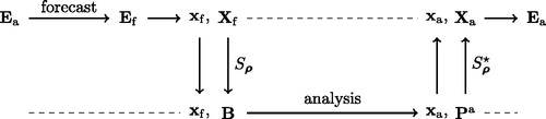21) is degenerate. The modified LEnSRF with this new update scheme follows the paradigm depicted in Fig. 1.

Fig. 1. Sequence of steps of a deterministic EnKF with covariance localisation, where the updated perturbations are obtained using the new scheme. Note that $\mathbf{B}$ and ${\mathbf{P}}^{\mathrm{a}}$ need not be fully computed.

With a view to efficiently minimising $\mathcal{L}(\mathbf{X}),$ let us compute its gradient with respect to $\mathbf{X}$ of size $N_{\mathrm{x}}\times N_{\mathrm{e}}.$ The variation of $\mathcal{L}(\mathbf{X})$ with respect to $\mathbf{X}$ is (23) $$\begin{array}{l}{\delta }_{\mathbf{X}}\mathcal{L}\left(\mathbf{X}\right)=\frac{1}{2}\left|\right|\mathbf{\Delta }\left|{|}_{\mathrm{F}}^{-2}{\delta }_{\mathbf{X}}\right|\left|\mathbf{\Delta }\right|{|}_{\mathrm{F}}^2=\frac{1}{2}\left|\right|\mathbf{\Delta }|{|}_{\mathrm{F}}^{-2}{\delta }_{\mathbf{X}}\text{Tr}\left[\mathbf{\Delta }{\mathbf{\Delta }}^{\top }\right]\\ =\left|\right|\mathbf{\Delta }|{|}_{\mathrm{F}}^{-2}\text{Tr}[\mathit{\rho }°\left\{\left({\delta }_{\mathbf{X}}\mathbf{X}\right){\mathbf{X}}^{\top }\right\}\mathbf{\Delta }\\ +\mathit{\rho }°\left\{\mathbf{X}{\left({\delta }_{\mathbf{X}}\mathbf{X}\right)}^{\top }\right\}\mathbf{\Delta }],\end{array}$$(23) where $\mathbf{\Delta }=\mathit{\rho }°\left(\mathbf{X}{\mathbf{X}}^{\top }\right)-{\mathbf{P}}^{\mathrm{a}}.$ Now, we use the identity (24) $$\text{Tr}\left[\left(\mathbf{A}°\mathbf{B}\right)·\mathbf{C}\right]=\text{Tr}\left[\mathbf{A}·\left({\mathbf{B}}^{\top }°\mathbf{C}\right)\right],$$(24) for any compatible $\mathbf{A},\mathbf{B},\mathbf{C}$ matrices and obtain: (25) $${\delta }_{\mathbf{X}}\mathcal{L}\left(\mathbf{X}\right)=2\left|\right|\mathbf{\Delta }|{|}_{\mathrm{F}}^{-2}\text{Tr}\left[{\left({\delta }_{\mathbf{X}}\mathbf{X}\right)}^{\top }\left(\mathit{\rho }°\mathbf{\Delta }\right)·\mathbf{X}\right].$$(25)

This yields the matrix gradient (26) $${\nabla }_{\mathbf{X}}\mathcal{L}\left(\mathbf{X}\right)=2\left|\right|\mathbf{\Delta }|{|}_{\mathrm{F}}^{-2}\left(\mathit{\rho }°\mathbf{\Delta }\right)·\mathbf{X},$$(26) i.e. the gradient of $\mathcal{L}(\mathbf{X})$ with respect to each component of matrix $\mathbf{X}.$ When implementing the new LEnSRF, we provide the gradient ${\nabla }_{\mathbf{X}}\mathcal{L}(\mathbf{X})$ as well as the value of $\mathcal{L}(\mathbf{X})$ to an off-the-shelf numerical optimisation code, such as L-BFGS-B (Byrd et al., 1995). Note that the function $\mathcal{L}(\mathbf{X})$ may not only have many global minima, but it may also have many local minima. As a consequence it may not be possible to find a global minimum with the L-BFGS-B method.

3.3. Parametrised minimisation

Instead of minimising $\mathcal{L}$ over $\mathbf{X}$ which has redundant degrees of freedom, we use an RQ decomposition of $\mathbf{X},$ which is obtained from a QR decomposition (Golub and van Loan, 2013) of ${\mathbf{X}}^{\top }:$ (27) $$\mathbf{X}=\mathbf{\Omega }\mathbf{U},$$(27) where $\mathbf{U}$ is an orthonormal matrix of size $N_{\mathrm{e}}\times N_{\mathrm{e}}$ and $\mathbf{\Omega }$ is a lower triangular (actually trapezoidal) matrix of size $N_{\mathrm{x}}\times N_{\mathrm{e}}.$ Hence, $\mathbf{X}{\mathbf{X}}^{\top }=\mathbf{\Omega }{\mathbf{\Omega }}^{\top }$ only depends on $\mathbf{\Omega }.$ The number of degrees of freedom of this parametrisation is that of $\mathbf{\Omega },$ which is (28) $$N_{\mathrm{e}}{N}_{\mathrm{x}}-N_{\mathrm{e}}\frac{N_{\mathrm{e}}-1}{2}=N_{\mathrm{e}}(N_{\mathrm{x}}-N_{\mathrm{e}})+N_{\mathrm{e}}\frac{N_{\mathrm{e}}+1}{2}.$$(28)

A parametrised minimisation can easily be implemented using the function (29) $$\mathcal{L}\left(\mathbf{\Omega }\right)=\hspace{0.17em}\text{ln}\hspace{0.17em}{\Vert \mathit{\rho }°\left(\mathbf{\Omega }{\mathbf{\Omega }}^{\top }\right)-{\mathbf{P}}^{\mathrm{a}}\Vert }_{\mathrm{F}}$$(29) and the gradient (30) $${\nabla }_{\mathbf{\Omega }}\mathcal{L}\left(\mathbf{\Omega }\right)=2\left|\right|\mathbf{\Delta }|{|}_{\mathrm{F}}^{-2}{\Pi }_{\mathbf{\Omega }}·\left(\mathit{\rho }°\mathbf{\Delta }\right)·\mathbf{\Omega },$$(30) where ${\Pi }_{\mathbf{\Omega }}$ is the projector that sets to 0 the upper triangular part of $\left(\mathit{\rho }°\mathbf{\Delta }\right)·\mathbf{\Omega }$ conformally to $\mathbf{\Omega },$ i.e. as in $\mathbf{\Omega }.$

We use this parametrised minimisation in all the numerical experiments. However, the plain method using the unparametrised minimisation on $\mathbf{X}$ works as well, although there is no guarantee to find the same local minimum because of the potential non-convexity of $\mathcal{L}(\mathbf{X}).$

In Appendix B, we address the question of the matrix norm choice in Eq. (21)(21) $$\begin{array}{c}{S}_{\mathit{\rho }}^{\star }\left({\mathbf{P}}^{\mathrm{a}}\right)=\underset{\text{rank}\left(\mathbf{X}\right)⩽N_{\mathrm{e}}-1}{\text{arg}\text{min}}\mathcal{L}\left(\mathbf{X}\right),\\ \text{with}\hspace{1em}\mathcal{L}\left(\mathbf{X}\right)=\hspace{0.17em}\text{ln}\hspace{0.17em}{\Vert S_{\mathit{\rho }}\left(\mathbf{X}\right)-{\mathbf{P}}^{\mathrm{a}}\Vert }_{\mathrm{F}},\end{array}$$(21) . In particular, we test the use of the spectral and nuclear matrix norms, and, more generally, of the Schatten p-norms. We found that these choices did not make much of a difference but that the choice of either the spectral or the nuclear norm, at the ends of the Schatten range, could lead to inaccurate numerical results.

Finally, coming back to the definition of $\mathcal{L}(\mathbf{X}),$ we have chosen to apply a logarithm function to the norm to level off the ups and downs of the function. Since the functions are non-convex, a quasi-Newton minimiser such as BFGS may behave differently in terms of convergence and local minima depending on the nature of the transformation. Hence, the log-transformation should not be considered totally innocuous. In practice, we found using the log-transform systematically beneficial.

3.4. Forecast of the $\mathit{\rho }°\left(\mathbf{X}{\mathbf{X}}^{\top }\right)$ representation

Because we have offered a novel view on the posterior perturbations and how they are generated in the analysis, we now need to examine how the forecast step of the scheme is affected by this change of standpoint. If not, there would be a risk of breaking the consistency in the forecast step of the cycle.

As previously explained at the end of Section 3.1, an asset of the LETKF approach is that the updated perturbations represent the dominant modes of the posterior error covariance matrix Eq. (15)(15) $${\mathbf{P}}^{\mathrm{a}}={\left({\mathbf{I}}_{\mathrm{x}}+\mathbf{B}{\mathbf{H}}^{\top }{\mathbf{R}}^{-1}\mathbf{H}\right)}^{-1}\mathbf{B}$$(15) . Hence, the forecast uncertainty must be approximated by the forecast of these modes. Nonetheless, by construction, the statistics of these modes before or after forecasting are only valid on local domains, i.e. for short spatial separations.

By contrast, with the new LEnSRF scheme, recognising that the posterior error covariance matrix is $\mathit{\rho }°\left({\mathbf{X}}_{\mathrm{a}}{\mathbf{X}}_{\mathrm{a}}^{\top }\right)$ makes forecasting more intricate. This representation $\mathit{\rho }°\left({\mathbf{X}}_{\mathrm{a}}{\mathbf{X}}_{\mathrm{a}}^{\top }\right)$ is meant to model statistics valid for larger spatial separations. How would one forecast this representation of the posterior error covariance matrix?

With the assumption that the error dynamics are linear, which would only be valid on short time scales, Bocquet (2016) has proposed a way to forecast $\mathit{\rho }°\left({\mathbf{X}}_{\mathrm{a}}{\mathbf{X}}_{\mathrm{a}}^{\top }\right).$ First, the ${\mathbf{X}}_{\mathrm{a}}$ are assumed to be genuine physical perturbations that are forecasted by the tangent linear resolvent ${\mathbf{M}}_{k+1:k}$ from time t_k to time $t_{k+1}:$ (31) $${\mathbf{X}}_{\mathrm{a}}^{(k+1)}={\mathbf{M}}_{k+1:k}{\mathbf{X}}_{\mathrm{a}}^{\left(k\right)}.$$(31)

The tangent linear model $\mathbf{M}{\prime }_k$ at t_k is defined by the expansion of the resolvent: ${\mathbf{M}}_{k+1:k}=\mathbf{I}+\mathbf{M}{\prime }_k(t_{k+1}-t_k)+o(t_{k+1}-t_k).$ Second, the localisation matrix should be made time-dependent and satisfy – in the time continuum limit – the following Liouville equation: (32) $$\frac{\partial \text{vec}\left(\mathit{\rho }\right)}{\partial t}=[\mathcal{K},\text{vec}(\mathit{\rho }\left)\right],\hspace{1em}\mathcal{K}=\mathbf{M}{\prime }_t\otimes \mathbf{I}+\mathbf{I}\otimes \left({\mathbf{M}}_t^{\prime }\right){}^{\top },$$(32) where $\text{vec}\mathit{\rho })$ is the vectorised $\mathit{\rho },$ a vector of size $N_{\mathrm{x}}^2$ whose entries are those of $\mathit{\rho }$ and ⊗ is the Kronecker product between two copies of the state space.

In the case where the dynamics can be approximated as hyperbolic, and in the limit where space is continuous, a closed-form equation can be obtained for $\rho (x_1,x_2,t)$ (see Eq. (A14) of Bocquet, 2016). If diffusion is present, there is no such closed-form equation. See also Kalnay et al. (2012); Desroziers et al. (2016) who have considered this issue in other contexts.

The key point is that in practice and for moderate forecast lead times, $\mathit{\rho }$ can roughly be assumed to be static. This is what will be used in the numerical experiments of Section 4. For larger $t_{k+1}-t_k,$ one could assume at the next order approximation that the localisation length used to obtain the prior at $t_{k+1}$ is larger than the one used in the perturbation update new scheme at t_k, because of an effective diffusion either generated by genuine diffusion or by averaged mixing advection (as stressed in the Appendix A of Bocquet, 2016).

This suggests that $\mathit{\rho }°\left({\mathbf{X}}_{\mathrm{f}}{\mathbf{X}}_{\mathrm{f}}^{\top }\right),$ obtained from the forecast perturbation matrix ${\mathbf{X}}_{\mathrm{f}}$ from ${\mathbf{X}}_{\mathrm{a}},$ is an acceptable approximation of the forecast error covariance matrix.

3.5. Numerical cost of computing the gradient and the cost function

In this section, we analyse the cost of computing the cost function and the gradient. Indeed, both would be required by a quasi-Newton minimiser and both involve ${\mathbf{P}}^{\mathrm{a}}.$ In the following, $\mathit{\rho }$ will be assumed either sparse or homogeneous. These are sine qua none conditions for the feasibility of covariance localisation with high-dimensional models.

3.5.1. Bottlenecks

The cost function $\mathcal{L}(\mathbf{X})$ requires computing (33) $$\begin{array}{l}\left|\right|\mathit{\rho }°\left(\mathbf{X}{\mathbf{X}}^{\top }\right)-{\mathbf{P}}^{\mathrm{a}}|{|}_{\mathrm{F}}^2\\ =\left|\right|\mathit{\rho }°\left(\mathbf{X}{\mathbf{X}}^{\top }\right)|{|}_{\mathrm{F}}^2+|\left|{\mathbf{P}}^{\mathrm{a}}\right|{|}_{\mathrm{F}}^2-2\text{Tr}\left\{\mathit{\rho }°\left(\mathbf{X}{\mathbf{X}}^{\top }\right){\mathbf{P}}^{\mathrm{a}}\right\}\\ =\text{Tr}\left\{\mathit{\rho }°\left(\mathbf{X}{\mathbf{X}}^{\top }\right)\left[\mathit{\rho }°\left(\mathbf{X}{\mathbf{X}}^{\top }\right)-2{\mathbf{P}}^{\mathrm{a}}\right]\right\}+\left|\right|{\mathbf{P}}^{\mathrm{a}}|{|}_{\mathrm{F}}^2\\ =\text{Tr}\left\{\mathbf{X}{\mathbf{X}}^{\top }\mathit{\rho }°\left[\mathit{\rho }°\left(\mathbf{X}{\mathbf{X}}^{\top }\right)-2{\mathbf{P}}^{\mathrm{a}}\right]\right\}+\left|\right|{\mathbf{P}}^{\mathrm{a}}|{|}_{\mathrm{F}}^2\\ =\text{Tr}\left\{{\mathbf{X}}^{\top }\mathit{\rho }°\left[\mathit{\rho }°\left(\mathbf{X}{\mathbf{X}}^{\top }\right)-2{\mathbf{P}}^{\mathrm{a}}\right]\mathbf{X}\right\}+\left|\right|{\mathbf{P}}^{\mathrm{a}}|{|}_{\mathrm{F}}^2.\end{array}$$(33)

As a consequence, the cost of evaluating $\mathcal{L}(\mathbf{X})$ is essentially driven by the evaluation of (34) $${\mathit{\rho }}_2°\left(\mathbf{X}{\mathbf{X}}^{\top }\right)·\mathbf{X}-2\left(\mathit{\rho }°{\mathbf{P}}^{\mathrm{a}}\right)·\mathbf{X},$$(34) where ${\mathit{\rho }}_2=\mathit{\rho }°\mathit{\rho }.$ The gradient Eq. (26)(26) $${\nabla }_{\mathbf{X}}\mathcal{L}\left(\mathbf{X}\right)=2\left|\right|\mathbf{\Delta }|{|}_{\mathrm{F}}^{-2}\left(\mathit{\rho }°\mathbf{\Delta }\right)·\mathbf{X},$$(26) unfolds as (35) $${\nabla }_{\mathbf{X}}\mathcal{L}\left(\mathbf{X}\right)=2\left|\right|\mathbf{\Delta }|{|}_{\mathrm{F}}^{-2}\left\{{\mathit{\rho }}_2°\left(\mathbf{X}{\mathbf{X}}^{\top }\right)·\mathbf{X}-\left(\mathit{\rho }°{\mathbf{P}}^{\mathrm{a}}\right)·\mathbf{X}\right\}.$$(35)

Thus, we need to consider the cost of evaluating both terms in the right-hand side. The normalising factor $\left|\right|\mathbf{\Delta }|{|}_{\mathrm{F}}^2$ coincides with Eq. (33)(33) $$\begin{array}{l}\left|\right|\mathit{\rho }°\left(\mathbf{X}{\mathbf{X}}^{\top }\right)-{\mathbf{P}}^{\mathrm{a}}|{|}_{\mathrm{F}}^2\\ =\left|\right|\mathit{\rho }°\left(\mathbf{X}{\mathbf{X}}^{\top }\right)|{|}_{\mathrm{F}}^2+|\left|{\mathbf{P}}^{\mathrm{a}}\right|{|}_{\mathrm{F}}^2-2\text{Tr}\left\{\mathit{\rho }°\left(\mathbf{X}{\mathbf{X}}^{\top }\right){\mathbf{P}}^{\mathrm{a}}\right\}\\ =\text{Tr}\left\{\mathit{\rho }°\left(\mathbf{X}{\mathbf{X}}^{\top }\right)\left[\mathit{\rho }°\left(\mathbf{X}{\mathbf{X}}^{\top }\right)-2{\mathbf{P}}^{\mathrm{a}}\right]\right\}+\left|\right|{\mathbf{P}}^{\mathrm{a}}|{|}_{\mathrm{F}}^2\\ =\text{Tr}\left\{\mathbf{X}{\mathbf{X}}^{\top }\mathit{\rho }°\left[\mathit{\rho }°\left(\mathbf{X}{\mathbf{X}}^{\top }\right)-2{\mathbf{P}}^{\mathrm{a}}\right]\right\}+\left|\right|{\mathbf{P}}^{\mathrm{a}}|{|}_{\mathrm{F}}^2\\ =\text{Tr}\left\{{\mathbf{X}}^{\top }\mathit{\rho }°\left[\mathit{\rho }°\left(\mathbf{X}{\mathbf{X}}^{\top }\right)-2{\mathbf{P}}^{\mathrm{a}}\right]\mathbf{X}\right\}+\left|\right|{\mathbf{P}}^{\mathrm{a}}|{|}_{\mathrm{F}}^2.\end{array}$$(33) .

Hence, for both the cost function and its gradient, we need to evaluate a first term in the form ${\mathit{\rho }}_2°\left(\mathbf{X}{\mathbf{X}}^{\top }\right)·\mathbf{X},$ and a second term in the form $\left(\mathit{\rho }°{\mathbf{P}}^{\mathrm{a}}\right)·\mathbf{X}.$

3.5.2. Efficient evaluation

It can be shown that (36) $$\mathit{\rho }°\left(\mathbf{X}{\mathbf{X}}^{\top }\right)·\mathbf{v}=\sum _{i=1}^{N_{\mathrm{e}}}{\mathbf{X}}_i°\left[\mathit{\rho }·\left({\mathbf{X}}_i°\mathbf{v}\right)\right],$$(36) where $\mathbf{X}$ is a matrix of size $N_{\mathrm{x}}\times N_{\mathrm{e}}$ and $\mathbf{v}$ a vector of size $N_{\mathrm{x}};$ ${\mathbf{X}}_i$ represents the i-th column of $\mathbf{X}.$ This can easily be shown by writing the matrix and vector indices explicitly (see e.g. Desroziers et al., 2014).

The numerical complexity of Eq. (36)(36) $$\mathit{\rho }°\left(\mathbf{X}{\mathbf{X}}^{\top }\right)·\mathbf{v}=\sum _{i=1}^{N_{\mathrm{e}}}{\mathbf{X}}_i°\left[\mathit{\rho }·\left({\mathbf{X}}_i°\mathbf{v}\right)\right],$$(36) is:

1. If $\mathit{\rho }$ is banded with a bandwidth of $N_{\mathrm{b}}:$ $\mathcal{O}\left(N_{\mathrm{e}}{N}_{\mathrm{x}}{N}_{\mathrm{b}}\right).$ Hence, the numerical complexity of computing the first term of Eqs. (34(34) $${\mathit{\rho }}_2°\left(\mathbf{X}{\mathbf{X}}^{\top }\right)·\mathbf{X}-2\left(\mathit{\rho }°{\mathbf{P}}^{\mathrm{a}}\right)·\mathbf{X},$$(34) ,35)(35) $${\nabla }_{\mathbf{X}}\mathcal{L}\left(\mathbf{X}\right)=2\left|\right|\mathbf{\Delta }|{|}_{\mathrm{F}}^{-2}\left\{{\mathit{\rho }}_2°\left(\mathbf{X}{\mathbf{X}}^{\top }\right)·\mathbf{X}-\left(\mathit{\rho }°{\mathbf{P}}^{\mathrm{a}}\right)·\mathbf{X}\right\}.$$(35) is $\mathcal{O}\left(N_{\mathrm{e}}^2{N}_{\mathrm{x}}{N}_{\mathrm{b}}\right)$ in this case.

2. If $\mathit{\rho }$ represents homogeneous correlations, corresponding to an invariance by translation: $\mathcal{O}\left(N_{\mathrm{e}}{N}_{\mathrm{x}}\hspace{0.17em}\text{ln}\hspace{0.17em}{N}_{\mathrm{x}}\right).$ Hence, the numerical complexity of computing the first term of Eqs. (34(34) $${\mathit{\rho }}_2°\left(\mathbf{X}{\mathbf{X}}^{\top }\right)·\mathbf{X}-2\left(\mathit{\rho }°{\mathbf{P}}^{\mathrm{a}}\right)·\mathbf{X},$$(34) ,35)(35) $${\nabla }_{\mathbf{X}}\mathcal{L}\left(\mathbf{X}\right)=2\left|\right|\mathbf{\Delta }|{|}_{\mathrm{F}}^{-2}\left\{{\mathit{\rho }}_2°\left(\mathbf{X}{\mathbf{X}}^{\top }\right)·\mathbf{X}-\left(\mathit{\rho }°{\mathbf{P}}^{\mathrm{a}}\right)·\mathbf{X}\right\}.$$(35) is $\mathcal{O}\left(N_{\mathrm{e}}^2{N}_{\mathrm{x}}\hspace{0.17em}\text{ln}\hspace{0.17em}{N}_{\mathrm{x}}\right)$ in this case.

Let us now consider the complexity of computing the second term. Assuming $\mathbf{P}$ is entirely known, we have (37) $$\begin{array}{l}{\left[\mathit{\rho }°\mathbf{P}·\mathbf{v}\right]}_n=\sum _m{\left[\mathit{\rho }\right]}_{n,m}{\left[\mathbf{P}\right]}_{n,m}{\left[\mathbf{v}\right]}_m=\sum _m{\left[\mathbf{P}\right]}_{n,m}{[{\mathit{\rho }}_n°\mathbf{v}]}_m\\ ={\mathbf{P}}_n{\mathit{\rho }}_n°\mathbf{v},\end{array}$$(37) where ${\mathit{\rho }}_n={[\mathit{\rho }]}_{\star ,n}$ and ${\mathbf{P}}_n={[\mathbf{P}]}_{n,\star }.$

If $\mathit{\rho }$ is banded, then the cost of the evaluation of ${\left[\mathit{\rho }°\mathbf{P}·\mathbf{v}\right]}_n$ is $\mathcal{O}\left(N_{\mathrm{b}}\right),$ so that the cost of evaluating $\mathit{\rho }°\mathbf{P}·\mathbf{v}$ is $\mathcal{O}\left(N_{\mathrm{x}}{N}_{\mathrm{b}}\right)$ and the cost of evaluating $\mathit{\rho }°\mathbf{P}·\mathbf{X}$ is $\mathcal{O}\left(N_{\mathrm{x}}{N}_{\mathrm{b}}{N}_{\mathrm{e}}\right).$ This cost is acceptable, i.e. it does not departs much from $\mathcal{O}(N_{\mathrm{x}}).$ However, it does not account for the cost of evaluating $\mathbf{P},$ which is the real issue when one considers ${\mathbf{P}}^{\mathrm{a}}.$

3.5.3. Mode expansion estimation of ${\mathbf{P}}^{\mathrm{a}}$

If we assume that we have extracted $N_{\mathrm{r}}$ modes stored in ${\widehat{\mathbf{X}}}_{\mathrm{a}}$ such that ${\mathbf{P}}^{\mathrm{a}}\approx {\widehat{\mathbf{X}}}_{\mathrm{a}}{\widehat{\mathbf{X}}}_{\mathrm{a}}^{\top }$ (the $N_{\mathrm{r}}$ largest EOFs of ${\mathbf{P}}^{\mathrm{a}}$), then the second term of Eqs. (34(34) $${\mathit{\rho }}_2°\left(\mathbf{X}{\mathbf{X}}^{\top }\right)·\mathbf{X}-2\left(\mathit{\rho }°{\mathbf{P}}^{\mathrm{a}}\right)·\mathbf{X},$$(34) ,35)(35) $${\nabla }_{\mathbf{X}}\mathcal{L}\left(\mathbf{X}\right)=2\left|\right|\mathbf{\Delta }|{|}_{\mathrm{F}}^{-2}\left\{{\mathit{\rho }}_2°\left(\mathbf{X}{\mathbf{X}}^{\top }\right)·\mathbf{X}-\left(\mathit{\rho }°{\mathbf{P}}^{\mathrm{a}}\right)·\mathbf{X}\right\}.$$(35) can be written $\mathit{\rho }°\left({\widehat{\mathbf{X}}}_{\mathrm{a}}{\widehat{\mathbf{X}}}_{\mathrm{a}}^{\top }\right)·\mathbf{X}$ which can also be computed using Eq. (36)(36) $$\mathit{\rho }°\left(\mathbf{X}{\mathbf{X}}^{\top }\right)·\mathbf{v}=\sum _{i=1}^{N_{\mathrm{e}}}{\mathbf{X}}_i°\left[\mathit{\rho }·\left({\mathbf{X}}_i°\mathbf{v}\right)\right],$$(36) since, typically, $N_{\mathrm{e}}⩽N_{\mathrm{r}}\ll N_{\mathrm{x}}.$ The cost of obtaining ${\widehat{\mathbf{X}}}_{\mathrm{a}}$ is the subject of Farchi and Bocquet (2019). Still assuming that we have ${\widehat{\mathbf{X}}}_{\mathrm{a}}$ such that ${\widehat{\mathbf{X}}}_{\mathrm{a}}{\widehat{\mathbf{X}}}_{\mathrm{a}}^{\top }\approx {\mathbf{P}}^{\mathrm{a}},$ the numerical complexity of computing the second term of Eqs. (34(34) $${\mathit{\rho }}_2°\left(\mathbf{X}{\mathbf{X}}^{\top }\right)·\mathbf{X}-2\left(\mathit{\rho }°{\mathbf{P}}^{\mathrm{a}}\right)·\mathbf{X},$$(34) ,35)(35) $${\nabla }_{\mathbf{X}}\mathcal{L}\left(\mathbf{X}\right)=2\left|\right|\mathbf{\Delta }|{|}_{\mathrm{F}}^{-2}\left\{{\mathit{\rho }}_2°\left(\mathbf{X}{\mathbf{X}}^{\top }\right)·\mathbf{X}-\left(\mathit{\rho }°{\mathbf{P}}^{\mathrm{a}}\right)·\mathbf{X}\right\}.$$(35) becomes $\mathcal{O}\left(N_{\mathrm{e}}{N}_{\mathrm{r}}{N}_{\mathrm{x}}{N}_{\mathrm{b}}\right)$ ($\mathcal{O}\left(N_{\mathrm{e}}{N}_{\mathrm{r}}{N}_{\mathrm{x}}\hspace{0.17em}\text{ln}\hspace{0.17em}{N}_{\mathrm{x}}\right)$) in case (i) (case (ii)), respectively. However, note that these computations can be embarrassingly parallelised, easily alleviating the cost by a factor of $N_{\mathrm{e}}$ or $N_{\mathrm{r}}$ on a parallel computer.

Note that Eqs. (9(9) $${\mathbf{X}}_{\mathrm{a}}={\mathbf{T}}_{\mathrm{x}}\mathbf{X}\hspace{1em}\text{with}\hspace{1em}{\mathbf{T}}_{\mathrm{x}}={\left({\mathbf{I}}_{\mathrm{x}}+\mathbf{B}{\mathbf{H}}^{\top }{\mathbf{R}}^{-1}\mathbf{H}\right)}^{-\frac{1}{2}}.$$(9) , 10(10) $${\mathbf{X}}_{\mathrm{a}}\approx {\mathbf{T}}_{\mathrm{x}}\mathbf{X}\hspace{1em}\text{with}\hspace{1em}{\mathbf{T}}_{\mathrm{x}}={\left({\mathbf{I}}_{\mathrm{x}}+{\mathbf{X}}_{\mathrm{r}}{\mathbf{Y}}_{\mathrm{r}}^{\top }{\mathbf{R}}^{-1}\mathbf{H}\right)}^{-\frac{1}{2}},$$(10) , 11(11) $$\begin{array}{l}{\mathbf{X}}_{\mathrm{a}}={\mathbf{T}}_{\mathrm{m}}\mathbf{X}\hspace{1em}\text{with}\hspace{1em}{\mathbf{T}}_{\mathrm{m}}={\mathbf{I}}_{\mathrm{x}}-{\mathbf{X}}_{\mathrm{r}}({\mathbf{I}}_{\mathrm{r}}+{\mathbf{Y}}_{\mathrm{r}}^{\top }{\mathbf{R}}^{-1}{\mathbf{Y}}_{\mathrm{r}}\\ {+{\left[{\mathbf{I}}_{\mathrm{r}}+{\mathbf{Y}}_{\mathrm{r}}^{\top }{\mathbf{R}}^{-1}{\mathbf{Y}}_{\mathrm{r}}\right]}^{\frac{1}{2}})}^{-1}{\mathbf{Y}}_{\mathrm{r}}^{\top }{\mathbf{R}}^{-1}\mathbf{H},\end{array}$$(11) ) may be irrelevant in computing the required ${\widehat{\mathbf{X}}}_{\mathrm{a}}$ since they do no strictly represent a mode expansion of ${\mathbf{P}}^{\mathrm{a}}.$ Instead, a systematic, variance-driven, expansion of ${\mathbf{P}}^{\mathrm{a}},$ as studied in Farchi and Bocquet (2019) would be required. The alternative is to use the modulation by Bishop and Hodyss (2009). But it could yield a substantially larger $N_{\mathrm{r}}$ and might be numerically costly.

3.5.4. Local evaluation of ${\mathbf{P}}^{\mathrm{a}}$

If the observations are assumed to be local, i.e. each one of them is only correlated to nearby model variables, then the main diagonals of ${\mathbf{P}}^{\mathrm{a}}$ can be estimated using local approximations, in a way similar to the strategy followed by the LETKF. Indeed, the LETKF is able to estimate rows or columns of ${\mathbf{P}}^{\mathrm{a}}$ using local analyses. Denoting ${\mathbf{P}}_n^{\mathrm{a}}\equiv {\left[{\mathbf{P}}^{\mathrm{a}}\right]}_n$ as the n-th column of ${\mathbf{P}}^{\mathrm{a}},$ one has (38) $${\mathbf{P}}_n^{\mathrm{a}}={\left[\mathbf{X}{\widehat{\mathbf{P}}}_n^{\mathrm{a}}{\mathbf{X}}^{\top }\right]}_n$$(38) where ${\widehat{\mathbf{P}}}_n^{\mathrm{a}}={\left({\mathbf{I}}_{\mathrm{e}}+{\mathbf{Y}}^{\top }{\mathbf{R}}_n^{-1}\mathbf{Y}\right)}^{-1}$ is the analysis error covariance matrix in ensemble space at site n and where ${\mathbf{R}}_n^{-1}$ is the tapered precision matrix with respect to site n.

Hence, the evaluation of ${\mathbf{P}}_n^{\mathrm{a}}$ is of complexity $\mathcal{O}\left(N_{\mathrm{b}}{N}_{\mathrm{e}}^2+N_{\mathrm{e}}^3\right),$ so that the evaluation of the entries of ${\mathbf{P}}^{\mathrm{a}}$ required in the evaluation of $\mathit{\rho }°{\mathbf{P}}^{\mathrm{a}}$ is $\mathcal{O}\left(N_{\mathrm{x}}{N}_{\mathrm{b}}{N}_{\mathrm{e}}^2\right),$ and a factor less if parallelisation is enforced.

Of course, one of the primary reasons for using covariance localisation is its ability to assimilate non-local observations. Hence, the assumption of locality made here defeats one of the key purpose of using covariance localisation. Nonetheless, we shall see that even with local observations, the update scheme developed in Section 3.2 can be beneficial.

4. Numerical experiments

4.1. Properties of the new perturbations

At first, we are interested in comparing the shape of the updated perturbations from a standard scheme compared to those of the new scheme. We also wish to explore how much can $\mathcal{L}({\mathbf{X}}_{\star })$ be rendered small, i.e. if there exists ${\mathbf{X}}_{\star }$ such that $\mathit{\rho }°\left({\mathbf{X}}_{\star }{\mathbf{X}}_{\star }^{\top }\right)\approx {\mathbf{P}}^{\mathrm{a}}.$ To that the end, we first consider a (random) Gaussian model of covariance $\mathbf{B}$ over a periodic one-dimensional domain for which $N_{\mathrm{x}}=400.$ The vector $\mathit{\sigma }$ of the standard deviations of $\mathbf{B}$ is obtained from a random draw from a log-normal distribution with Gaussian covariance matrix of correlation length $L_{\mathrm{v}}=10.$ The correlation matrix $\mathbf{C}$ associated to $\mathbf{B}$ is built from the piece-wise rational Gaspari–Cohn (Gaspari and Cohn, 1999) function (hereafter referred to as the GC function) with correlation length parameter $L_{\mathrm{c}}=10.$ From these definitions, we have $\mathbf{B}=\mathbf{\Sigma }\mathbf{C}\mathbf{\Sigma }$ where $\mathbf{\Sigma }=\text{diag}(\mathit{\sigma })$ is the diagonal matrix of the standard deviations.

We compare the shape of $N_{\mathrm{e}}=8$ perturbations, whose sample covariance matrix may be regularised using a correlation matrix $\mathit{\rho }$ built with the GC function with a localisation length parameter $L_{\mathit{\rho }}=10.$ The perturbations are generated by

1. random draws ${\mathbf{X}}_{\mathrm{e}}$ from the covariance matrix $\mathbf{B}.$ We associate to them the sample covariance matrix ${\mathbf{P}}^{\mathrm{e}}={\mathbf{X}}_{\mathrm{e}}{\mathbf{X}}_{\mathrm{e}}^{\top }$ and its regularised counterpart ${\mathbf{P}}_{\mathit{\rho }}^{\mathrm{e}}=\mathit{\rho }°{\mathbf{P}}^{\mathrm{e}};$

2. extracting the main $N_{\mathrm{e}}$ modes, $\widehat{\mathbf{X}}$ of $\mathbf{B}.$ We associate to them the sample covariance matrix $\widehat{\mathbf{P}}=\widehat{\mathbf{X}}{\widehat{\mathbf{X}}}^{\top },$ and its regularised counterpart ${\widehat{\mathbf{P}}}_{\mathit{\rho }}=\mathit{\rho }°\widehat{\mathbf{P}};$

3. extracting $N_{\mathrm{e}}$ modes using the new scheme, ${\mathbf{X}}_{\star }=S_{\mathit{\rho }}^{\star }\left(\mathbf{B}\right).$ We associate to them the sample covariance matrix ${\mathbf{P}}^{\star }={\mathbf{X}}_{\star }{\mathbf{X}}_{\star }^{\top },$ and its regularised counterpart ${\mathbf{P}}_{\mathit{\rho }}^{\star }=\mathit{\rho }°{\mathbf{P}}^{\star }.$ The starting point of the minimisation (first guess) is chosen to be $\widehat{\mathbf{X}}.$

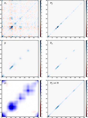
Figure 2 displays, for a single realisation of the covariance model, the true covariance model $\mathbf{B},$ the sample covariance matrices ${\mathbf{P}}^{\mathrm{e}},\widehat{\mathbf{P}},{\mathbf{P}}^{\star },$ and the regularised sample covariance matrices ${\mathbf{P}}_{\mathit{\rho }}^{\mathrm{e}},{\widehat{\mathbf{P}}}_{\mathit{\rho }}$ and ${\mathbf{P}}_{\mathit{\rho }}^{\star }.$

Fig. 2. Density plots of the covariance matrices discussed in the text, except for ${\mathbf{P}}^{•}$ and ${\mathbf{P}}_{\mathit{\rho }}^{•}.$ The raw sample covariance matrices are on the left, while the regularised (by localisation) sample covariance matrix are on the right. The true covariance matrix ($\mathbf{B}$) cannot be visually discriminated from ${\mathbf{P}}_{\mathit{\rho }}^{\star }$ (bottom-right corner).

For the same realisation, Fig. 3 displays the perturbations ${\mathbf{X}}_{\mathrm{e}},\widehat{\mathbf{X}},$ ${\mathbf{X}}_{\star }.$ We also consider a second optimal solution where the first guess is ${\mathbf{X}}_{\mathrm{e}},$ which yields another set of perturbations, ${\mathbf{X}}_{•}$ in order to investigate the dependence on the starting point of the minimisation.

Fig. 3. Plot of the $N_{\mathrm{e}}=8$ perturbation sets: ${\mathbf{X}}_{\mathrm{e}},\widehat{\mathbf{X}},{\mathbf{X}}_{\star }$ and ${\mathbf{X}}_{•},$ with respect to the grid-point index.

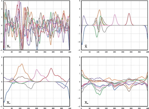
It is clear from Fig. 2 that ${\mathbf{P}}^{\star }$ seems unphysical with rather long-range correlations, but that ${\mathbf{P}}_{\mathit{\rho }}^{\star }$ is, as a result of its construction, a remarkably close match to $\mathbf{B}.$ $\widehat{\mathbf{P}}$ seems a rather good approximation of $\mathbf{B}.$ However, it is clear that ${\widehat{\mathbf{P}}}_{\mathit{\rho }}$ has a thinner structure along the diagonal than $\mathbf{B},$ which can be seen as a manifestation of the double application of localisation. These visual impressions on a single realisation are confirmed by computing the Frobenius norm of the difference between the true covariance matrix $\mathbf{B}$ and either the sample covariance matrix or the regularised sample covariance matrix. The norm is averaged over 10³ realisations. The results are reported in Table 1. In particular, either ${\mathbf{P}}_{\mathit{\rho }}^{\star }$ or ${\mathbf{P}}_{\mathit{\rho }}^{•}$ are a close match to $\mathbf{B},$ and their residual discrepancy to $\mathbf{B}$ as measured by these matrix norms are very small and similar, though not identical.

Table 1. Averaged Frobenius norm that measures the discrepancy between the target covariance matrix $\mathbf{B}$ and several raw (first row) or regularised (second row) sample error covariance matrices.

Norm	${\mathbf{P}}^{\mathrm{e}}$	$\widehat{\mathbf{P}}$	${\mathbf{P}}^{\star }$	${\mathbf{P}}^{•}$
$\left|\right|*-\mathbf{B}|{|}_{\mathrm{F}}$	194	50	331	335
$\left|\right|{*}_{\mathit{\rho }}-\mathbf{B}|{|}_{\mathrm{F}}$	49	49	0.05	0.06

For the sake of comparison note that, on average, $\left|\right|\mathbf{B}|{|}_{\mathrm{F}}=87.$

As seen in Fig. 3 the perturbations $\widehat{\mathbf{X}}$ are rather local and peaked functions, which could be expected since they represent the first EOFs of $\mathbf{B}.$ The perturbations ${\mathbf{X}}_{\star }$ obtained with the new scheme starting with $\widehat{\mathbf{X}}$ are much broader functions with a larger support. This is due to the weaker constraints imposed on these modes. However, they remain partially localised, in that they partly vanish on the domain. The perturbations ${\mathbf{X}}_{•}$ obtained with the new scheme but starting with ${\mathbf{X}}_{\mathrm{e}}$ are also broad functions. However, as opposed to ${\mathbf{X}}_{\star },$ they do not partially vanish, and are barely local. This shows that $S_{\mathit{\rho }}(\mathbf{B})$ indeed represents a set of potentially distinct solutions and that the solution to which the minimisation converges captures traits of the starting perturbations.

4.2. Accuracy of the scheme

4.2.1. Lorenz–96 model

The performance of the new scheme is tested in a mildly nonlinear configuration of the discrete 40-variable one-dimensional Lorenz–96 (L96) model (Lorenz and Emanuel, 1998), with the standard forcing F = 8. The corresponding ordinary differential equations defined on a periodic domain are for $n=1,\dots ,N_{\mathrm{x}}=40:$ (39) $$\frac{\mathrm{d}{x}_n}{\mathrm{d}t}=(x_{n+1}-x_{n-2})x_{n-1}-x_n+F.$$(39) where $x_{N_{\mathrm{x}}+1}=x_1,x_0=x_{N_{\mathrm{x}}}$ and $x_{-1}=x_{N_{\mathrm{x}}-1}.$ These equations are integrated using a fourth-order Runge–Kutta scheme with the time step $\delta t=0.05$ in L96 time unit.

We consider twin experiments where synthetic observations are generated from the true model trajectory every $\Delta t=0.05.$ The observation operator is chosen to be $\mathbf{H}={\mathbf{I}}_{\mathrm{x}};$ in particular, the model is fully observed. The observation errors are Gaussian with distribution $\mathcal{N}(\mathbf{0},\mathbf{R})$ and observation error covariance matrix $\mathbf{R}={\mathbf{I}}_{\mathrm{x}}.$ A sparse observation network configuration will be studied in Section 4.3.

We test the following data assimilation schemes:

1. The standard LETKF as defined by Hunt et al. (2007).

2. The LEnSRF as defined in Section 2.3.2. The ${\mathbf{T}}_{\mathrm{x}}$ matrices are computed exactly in this low-order setup. Section 2.4 would be used for higher dimensional models.

3. The new LEnSRF with the new updating scheme. The ${\mathbf{P}}^{\mathrm{a}}$ matrices are computed exactly in this low-order setup. The strategies defined in Section 3.5 would be used for higher dimensional models. We choose to start the minimisation of $\mathcal{L}(\mathbf{X})$ from the background perturbations, the natural incremental standpoint.

When $N_{\mathrm{e}}-1⩽14,$ which corresponds to the size of the unstable and neutral subspace of this model, localisation is mandatory to avoid divergence of the filters (Bocquet and Carrassi, 2017). The localisation function used to build the localisation matrix for covariance localisation (LEnSRF) or for tapering the observation error precision matrix (LETKF) is the GC function. In order to achieve a good (though approximate) match between the LETKF and the LEnSRF, the tapering of the perturbations in the LETKF, known to be equivalent to the tapering of the precision matrix, is carried out using the square root of the GC function (Sakov and Bertino, 2011). The performance of the algorithms are mainly assessed by the time-averaged root mean square error (RMSE) between the analysis and the truth. The multiplicative inflation (in the range $\lambda \in [1,1.08]$), which is applied to the prior perturbations, and the localisation radius (in the range $r\in [4,38]$ sites) are optimally tuned so as to yield the lowest RMSE. Random rotations are applied after each update (Sakov and Oke, 2008b). It does marginally improve the RMSE scores for large values of $N_{\mathrm{e}}.$

For each configuration, 10 data assimilation experiments are run. Each run is $2\times {10}^4$ cycle-long after a spin-up of $2\times {10}^3$ cycles. All statistics are averaged over these 10 runs. The results are displayed in the left column of Fig. 4.

Fig. 4. Comparison of the LETKF, the LEnSRF and the LEnSRF with the new update scheme, applied to the L96 model (left column) and to the KS model (right column). The RMSE, optimal localisation and optimal inflation are plotted as functions of the ensemble size $N_{\mathrm{e}}.$

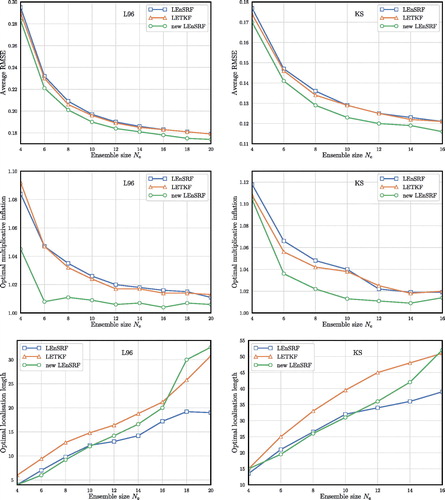
First, the LETKF and the LEnSRF show similar RMSEs, and optimal inflation for all ensemble sizes, but the LETKF has the edge for both the RMSE and the inflation. The optimal localisation lengths for the three schemes are similar, in particular thanks to the approximate correspondence between the way the observation precision matrix is tapered in the LETKF and the way the background error covariance is tapered in the LEnSRF. Nonetheless the localisation length of the traditional LEnSRF is smaller than the other two EnKFs, especially for larger ensemble sizes.

Second, the new LEnSRF with the new update shows lower RMSEs, and significantly lower optimal inflation than the other two schemes. The improvement in the RMSE is in the range $3\%-6\%,$ which is significant in these very well-tuned and documented configurations, where such gain is very difficult to obtain.

Focusing on the multiplicative inflation requirement, we have computed the RMSE as a function of the inflation, with the localisation length optimally tuned so as to minimise the RMSE, for three ensemble sizes $N_{\mathrm{e}}=4,8,16.$ The results are plotted in the left column in Fig. 5.

Fig. 5. Time-averaged RMSE as a function of the multiplicative inflation, the localisation length being tuned so as to minimise the RMSE. The L96 results are displayed on the left panels while the KS results are shown on the right panels, for $N_{\mathrm{e}}=4,8,16.$ An absent marker means that at least one of the 10 sample runs has diverged from the truth.

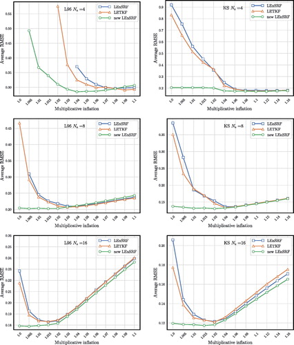
It shows that the requirement of the new LEnSRF for inflation is actually very small. In the case $N_{\mathrm{e}}=8,16$ inflation is barely needed, while the extreme case $N_{\mathrm{e}}=4$ does show a need for inflation but much smaller than that of the LEnSRF and LETKF. This points to the robustness of the new LEnSRF.

By construction, $S_{\mathit{\rho }}\left(S_{\mathit{\rho }}^{\star }({\mathbf{P}}^{\mathrm{a}})\right)$ as implicitly relied upon in the new LEnSRF is a better match to ${\mathbf{P}}^{\mathrm{a}}$ than $S_{\mathit{\rho }}\left({\mathbf{X}}_{\mathrm{a}}\right)$ where ${\mathbf{X}}_{\mathrm{a}}$ is defined by Eq. (9)(9) $${\mathbf{X}}_{\mathrm{a}}={\mathbf{T}}_{\mathrm{x}}\mathbf{X}\hspace{1em}\text{with}\hspace{1em}{\mathbf{T}}_{\mathrm{x}}={\left({\mathbf{I}}_{\mathrm{x}}+\mathbf{B}{\mathbf{H}}^{\top }{\mathbf{R}}^{-1}\mathbf{H}\right)}^{-\frac{1}{2}}.$$(9) as used in the LEnSRF. This might explain the lesser requirement for multiplicative inflation.

We speculate that this lesser need for multiplicative inflation in the new LEnSRF may also be interpreted as a reduced imbalance of the updated perturbations. If true, this implies that for the L96 model in this standard setup, the residual inflation required in the LETKF and LEnSRF does not so much originate from the sampling errors but from the imbalance generated by localisation. This, however, can only be validated on physically more complex, $2-$ or $3-$dimensional models, beyond the scope of this paper.

4.2.2. Kuramoto–Sivashinsky model

We have performed similar experiments with the Kuramoto–Sivashinsky (KS) model (Kuramoto and Tsuzuki, 1975, 1976; Sivashinsky, 1977). It is defined by the partial differential equation (40) $$\frac{\partial u}{\partial t}=-u\frac{\partial u}{\partial x}-\frac{{\partial }^{2}u}{\partial x^2}-\frac{{\partial }^{4}u}{\partial x^4}$$(40) over the domain $x\in [0,32\pi ].$ As opposed to the L96 model, the KS model is continuous though numerically discretised in Fourier modes. It is characterised by sharp density gradients so that it may be expected that local EnKFs are prone to imbalance. We have chosen $N_{\mathrm{x}}=128$ modes, corresponding to $N_{\mathrm{x}}=128$ collocation grid points. The model is integrated using the ETDRK4 scheme (Kassam and Trefethen, 2005) with the time step $\delta t=0.50$ in time unit of the KS model. Synthetic observations are collected every $\Delta t=1$ on all collocation grid points. The observation operator is chosen to be $\mathbf{H}={\mathbf{I}}_{\mathrm{x}};$ in particular, the model is fully observed. The observation errors are Gaussian with distribution $\mathcal{N}(\mathbf{0},\mathbf{R})$ and observation error covariance matrix $\mathbf{R}={\mathbf{I}}_{\mathrm{x}}.$ Like for the L96 model experiments, the localisation matrix used in either the LEnSRFs or the LETKF is built from the GC function, and random rotations are applied after each update. The performance of the algorithms are assessed by the time-averaged analysis RMSE as well. The multiplicative inflation (in the range $\lambda \in [1,1.16]$) and the localisation radius (in the range $r\in [10,80]$ sites) are optimally tuned so as to yield the best RMSE.

For each configuration, 10 data assimilation experiments are run. Each run is $2\times {10}^4$ cycle-long after a spin-up of $2\times {10}^3$ cycles. All statistics are averaged over these 10 runs. Note that for $N_{\mathrm{e}}-1⩽14,$ which corresponds to the size of the unstable and neutral subspace of this model, localisation is mandatory to avoid divergence of the filters. The results are displayed in the right column of Fig. 4.

The results are very similar to those of the L96 model. The LEnSRF with the new update scheme outperforms the other two schemes, with a much lower need for inflation, and optimal localisation lengths similar to that of the LEnSRF without the new update scheme. For this model, the optimal localisation length for the LETKF is however larger than for both LEnSRFs.

The requirement for multiplicative inflation is further studied similarly to the L96 case. The right column of Fig. 5 shows the RMSE as a function of multiplicative inflation for optimally tuned localisation length and for $N_{\mathrm{e}}=4,8,16.$ Again, it shows that the need for inflation is substantially reduced and not really needed for $N_{\mathrm{e}}=8,16,$ and even $N_{\mathrm{e}}=4,$ demonstrating the robustness of the new LEnSRF.

4.3. Sparse and infrequent observations

Localisation schemes can behave differently in presence of sparse and inhomogeneous observations. Moreover, we have conjectured that the new perturbations update scheme could generate an ensemble with less imbalance (closer to the attractor), which could be evidenced with longer forecasts in the EnKF than those considered so far. Hence, in this section, we consider:

1. A first set of experiments where the state vector entries are uniformly and randomly observed with a fixed density $N_{\mathrm{y}}/N_{\mathrm{x}},$ which is varied from 0.25 to 1. Specifically, at each observation time, $N_{\mathrm{y}}$ grid cells are randomly selected (without replacement) over the total $N_{\mathrm{x}}$ grid cells and the observation operator $\mathbf{H}$ directly yields the value of the state vector at each of these grid cells. The observations are collected every $\Delta t=0.05$ time unit.

2. A second set of experiments where the observations are spatially densely observed ($\mathbf{H}={\mathbf{I}}_{\mathrm{x}}$) but with a fixed time step which is varied from $\Delta \mathrm{t}=0.05$ to the much less frequent $\Delta \mathrm{t}=0.40.$ For such long forecast, the more accurate local iterative ensemble Kalman filter (IEnKF) would yield better RMSEs (Bocquet, 2016), but applying the new update scheme to the IEnKF with localisation is outside the scope of this paper.

We choose to focus on the L96 model and an ensemble size of $N_{\mathrm{e}}=8$ and $\mathbf{R}={\mathbf{I}}_{\mathrm{y}}.$ In both experiments, the localisation length is optimally tuned so as to minimise the RMSE.

For the first set of experiments, we plot in Fig. 6 the time-averaged analysis RMSE (left panel) and the optimal inflation (right panel) required to minimise this RMSE as a function of the fixed density of observations $N_{\mathrm{y}}/N_{\mathrm{x}},$ for the three EnKFs considered in the previous experiments. The localisation length is optimally tuned so as to minimise the RMSE.

Fig. 6. Comparison of the LETKF, the LEnSRF and the LEnSRF with the new update scheme, applied to the L96 model, for a fixed ensemble size $N_{\mathrm{e}}=8$ and a fixed observation time step $\Delta t=0.05.$ The RMSE (left panel) and the optimal inflation (right panel) are plotted as functions of the observation density $N_{\mathrm{y}}/N_{\mathrm{x}}.$

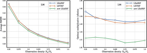
The results are very similar to those obtained in the previous subsection: the new LEnSRF scheme yields a typical 5% improvement in the RMSE, while using a significantly lower multiplicative inflation. In the left panel of Fig. 8, the RMSEs of the three schemes for $N_{\mathrm{e}}=8,\Delta t=0.05$ and $N_{\mathrm{y}}/N_{\mathrm{x}}=0.50,$ are plotted as a function of the multiplicative inflation, while the localisation length is optimally tuned so as to minimise the RMSE. Again, this emphasises the little need for multiplicative inflation of the new LEnSRF.

For the second set of experiments, we plot in Fig. 7 the time-averaged RMSE (left panel) and the optimal inflation (right panel) required to minimise this RMSE as a function of the time interval between observations $\Delta t,$ for the three considered EnKFs. Again, the new LEnSRF yields smaller RMSEs than the classical LEnSRF and the LETKF. As $\Delta t$ increases, the multiplicative inflation required to compensate for the error generated by sampling errors increases too. This is known to be due to the increased nonlinearity of the forecast (Bocquet et al., 2015; Raanes et al., 2019). The optimal multiplicative inflation required by the new LEnSRF does increase with $\Delta t$ but remains significantly smaller than the one required by the other two EnKFs. Differently from the previous numerical experiments, the LETKF outperforms the classical LEnSRF and its RMSE curve gets closer to that of the new LEnSRF with larger $\Delta t.$ This supports our claim made in Sect. 3.1 that the LETKF might generate better forecast ensembles.

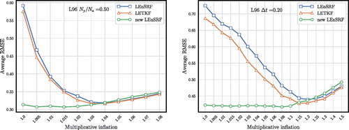
In the right panel of Fig. 8, the RMSEs of the three schemes for $N_{\mathrm{e}}=8,\Delta t=0.20$ and $N_{\mathrm{y}}/N_{\mathrm{x}}=1,$ are plotted as a function of the multiplicative inflation, while the localisation length is optimally tuned so as to minimise the RMSE. This shows that the new LEnSRF can yield good RMSE scores even with small inflation factors and for longer forecasts.

Fig. 7. Comparison of the LETKF, the LEnSRF and the LEnSRF with the new update scheme, applied to the L96 model, for a fixed ensemble size $N_{\mathrm{e}}=8$ and a fully observed model. The RMSE (left panel) and the optimal inflation (right panel) are plotted as functions of the observation time step $\Delta t.$

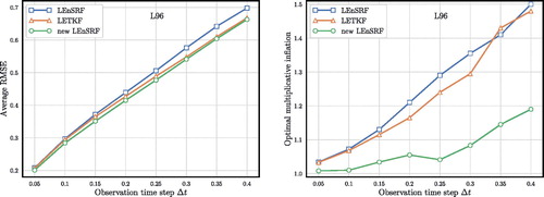
Fig. 8. Time-averaged RMSE for the L96 model as a function of the multiplicative inflation, the localisation length being tuned so as to minimise the RMSE in the two configurations where the observations are sparser ($N_{\mathrm{y}}/N_{\mathrm{x}}=0.50,$ left panel) and where the observations are infrequent ($\Delta t=0.20,$ right panel). $N_{\mathrm{e}}=8$ in both configurations.

We have also computed the ratio of the analysis RMSE over the ensemble spread, as $\Delta t$ is increased, the multiplicative inflation and localisation length being tuned so as the minimise the RMSE. The new LEnSRF and the LETKF behave quite similarly with a ratio progressively increasing from 1 to 1.10 when $\Delta t$ goes from 0.05 to 0.40. Quite differently, the classical LEnSRF shows a ratio that increases from 1 to 1.30 when $\Delta t$ goes from 0.05 to 0.40. Again, this supports the idea that the forecast ensembles of the new LEnSRF and the LETKF are of better quality than those of the classical LEnSRF.

Note that we have also considered time-averaged forecast RMSE and spread for a range of forecast lead times. They follow the same trend as the analysis RMSE and analysis spread but are progressively amplified with increasing lead time.

All of these experiments have also been conducted with the KS model. The results are qualitatively very similar and yield the same conclusions for both the sparse and infrequent observation experiments.

5. Conclusions

In this paper, we have looked back at the perturbation update scheme in the EnKFs based on covariance localisation. We have argued that updated perturbations in the local EnKFs based on covariance localisation do not represent the main modes of the analysis error covariance matrix, in contrast to the updated perturbations of the LETKF. In particular, we have focused on the LEnSRF. We have explained why Eq. (9)(9) $${\mathbf{X}}_{\mathrm{a}}={\mathbf{T}}_{\mathrm{x}}\mathbf{X}\hspace{1em}\text{with}\hspace{1em}{\mathbf{T}}_{\mathrm{x}}={\left({\mathbf{I}}_{\mathrm{x}}+\mathbf{B}{\mathbf{H}}^{\top }{\mathbf{R}}^{-1}\mathbf{H}\right)}^{-\frac{1}{2}}.$$(9) still is, on theoretical grounds, a good substitute for generating these perturbations.

Using these considerations, we have proposed a perturbation update scheme potentially more consistent in the sense that the perturbations $\mathbf{X}$ are related to the error covariance matrix by $\mathbf{P}\approx \mathit{\rho }°\left(\mathbf{X}{\mathbf{X}}^{\top }\right)$ throughout the EnKF scheme. It consists in getting one solution of the minimisation problem Eq. (21)(21) $$\begin{array}{c}{S}_{\mathit{\rho }}^{\star }\left({\mathbf{P}}^{\mathrm{a}}\right)=\underset{\text{rank}\left(\mathbf{X}\right)⩽N_{\mathrm{e}}-1}{\text{arg}\text{min}}\mathcal{L}\left(\mathbf{X}\right),\\ \text{with}\hspace{1em}\mathcal{L}\left(\mathbf{X}\right)=\hspace{0.17em}\text{ln}\hspace{0.17em}{\Vert S_{\mathit{\rho }}\left(\mathbf{X}\right)-{\mathbf{P}}^{\mathrm{a}}\Vert }_{\mathrm{F}},\end{array}$$(21) . The updated perturbations are expected to be more accurate in forming short spatial separation sample covariances because less constraints are exerted on large separation sample covariances. Since we can compute the gradient of the function to be minimised, the solution can be obtained using an off-the-shelf quasi-Newton algorithm. The evaluation of the function and its gradient requires knowledge of $\mathit{\rho }°{\mathbf{P}}^{\mathrm{a}},$ hence a partial knowledge of ${\mathbf{P}}^{\mathrm{a}},$ which is one difficulty of the method. Depending on the problem, its geometry and dimension, such knowledge could be obtained through mode expansion or through local estimations of ${\mathbf{P}}^{\mathrm{a}}.$

We have tested this idea and defined a new LEnSRF with the new perturbation update scheme. We have compared it numerically to the LETKF and to a vanilla LEnSRF based on an implementation of Eq. (9)(9) $${\mathbf{X}}_{\mathrm{a}}={\mathbf{T}}_{\mathrm{x}}\mathbf{X}\hspace{1em}\text{with}\hspace{1em}{\mathbf{T}}_{\mathrm{x}}={\left({\mathbf{I}}_{\mathrm{x}}+\mathbf{B}{\mathbf{H}}^{\top }{\mathbf{R}}^{-1}\mathbf{H}\right)}^{-\frac{1}{2}}.$$(9) , using two low-order one-dimensional models: the discrete 40-variable Lorenz–96 model and a 128-variable spectral discretisation of the continuous Kuramoto–Sivashinsky model. We have shown that for both models, the requirement for residual multiplicative inflation still needed in spite of localisation is much weaker with the new LEnSRF than with both the LETKF and the LEnSRF. For large enough ensemble sizes, the new LEnSRF actually performs very well without any inflation. This weaker requirement for inflation stems from a better consistency of the analysis error covariance matrix as inferred by the updated perturbation to the actual one. We conjecture that it could be physically interpreted as a much weaker imbalance generated by the new update scheme. Moreover, there is an accuracy improvement of up to 6% in the analysis RMSE in mildly nonlinear conditions, which is significant in these very well-tuned configurations. The RMSE/spread score is shown to be closer to 1 for the LETKF and the new LEnSRF than for the vanilla LEnSRF. These results have been confirmed and further strengthened in sparse and infrequent observation network configurations.

We plan on testing this new scheme on two-dimensional models and more sophisticated physics. We also plan to study the potential benefit of such update scheme in an hybrid setup (i.e. using hybrid covariances).

Acknowledgments

The authors are thankful to two anonymous reviewers for their insightful comments and suggestions. CEREA is a member of Institute Pierre-Simon Laplace (IPSL).

Notes

1 There are actually two main definitions of a matrix square root. The main one in mathematics defines a square root of $\mathbf{A}$ as a solution $\mathbf{B}$ of ${\mathbf{B}}^2=\mathbf{A}.$ An alternate definition, sometimes used in geosciences and which gave its name to the square root filters, is $\mathbf{B}$ defined as a solution of $\mathbf{B}{\mathbf{B}}^{\top }=\mathbf{A}.$ In both cases, the solution is usually not being unique. Moreover, these definitions are incompatible so that we have to make a clear choice. The choice that we make (i) complies with the mathematical definition and (ii) unambiguously select one solution when there at least one.

2 It is actually known to be NP-hard.

3 It generalises the classical Cauchy’s intregral formula using the Jordan decomposition of matrices. See for instance, Eq. (2.7) in Kassam and Trefethen (2005).

Appendix A: left-transform update in perturbation space and in observation space

In this appendix, we (i) give an alternate and rigorous derivation to the heuristic one proposed in appendix B of Bocquet (2016), (ii) re-derive Eq. (11)(11) $$\begin{array}{l}{\mathbf{X}}_{\mathrm{a}}={\mathbf{T}}_{\mathrm{m}}\mathbf{X}\hspace{1em}\text{with}\hspace{1em}{\mathbf{T}}_{\mathrm{m}}={\mathbf{I}}_{\mathrm{x}}-{\mathbf{X}}_{\mathrm{r}}({\mathbf{I}}_{\mathrm{r}}+{\mathbf{Y}}_{\mathrm{r}}^{\top }{\mathbf{R}}^{-1}{\mathbf{Y}}_{\mathrm{r}}\\ {+{\left[{\mathbf{I}}_{\mathrm{r}}+{\mathbf{Y}}_{\mathrm{r}}^{\top }{\mathbf{R}}^{-1}{\mathbf{Y}}_{\mathrm{r}}\right]}^{\frac{1}{2}})}^{-1}{\mathbf{Y}}_{\mathrm{r}}^{\top }{\mathbf{R}}^{-1}\mathbf{H},\end{array}$$(11) , (iii) proves Eq. (12)(12) $$\begin{array}{l}{\mathbf{X}}_{\mathrm{a}}={\mathbf{T}}_{\mathrm{y}}\mathbf{X}\hspace{1em}\text{with}\hspace{1em}{\mathbf{T}}_{\mathrm{y}}={\mathbf{I}}_{\mathrm{x}}-{\mathbf{X}}_{\mathrm{r}}{\mathbf{Y}}_{\mathrm{r}}^{\top }(\mathbf{R}+{\mathbf{Y}}_{\mathrm{r}}{\mathbf{Y}}_{\mathrm{r}}^{\top }{+\mathbf{R}{\left[{\mathbf{I}}_{\mathrm{y}}+{\mathbf{R}}^{-1}{\mathbf{Y}}_{\mathrm{r}}{\mathbf{Y}}_{\mathrm{r}}^{\top }\right]}^{\frac{1}{2}})}^{-1}\mathbf{H},\end{array}$$(12) and (iv) shows how this latter result generalises the filter formalism developed in Anderson (2003).

Let $\mathbf{A}$ be a matrix of size $N_{\mathrm{x}}\times N_{\mathrm{e}}$ and $\mathbf{B}$ be a matrix of size $N_{\mathrm{e}}\times N_{\mathrm{x}}.$ For any $z\in \mathbb{C}$ which is an eigenvalue of neither $\mathbf{AB}$ nor $\mathbf{BA},$ we have the identity: (A1) $${\left(z{\mathbf{I}}_{\mathrm{x}}-\mathbf{AB}\right)}^{-1}=\frac{1}{z}\left\{{\mathbf{I}}_{\mathrm{x}}+\mathbf{A}{\left(z{\mathbf{I}}_{\mathrm{e}}-\mathbf{BA}\right)}^{-1}\mathbf{B}\right\},$$(A1) which can be straightforwardly proven by showing that the product of the right-hand side with the inverse of the left-hand side is ${\mathbf{I}}_{\mathrm{x}}$ and the product of the inverse of the left-hand side with the right-hand side is ${\mathbf{I}}_{\mathrm{x}}.$

Let f be a function such that $f(0)=1,$ and which is analytic in a connected domain $\mathcal{D}$ of contour $\mathcal{C}$ in the complex plane $\mathbb{C}$ which encloses the eigenvalues of both $\mathbf{AB}$ and $\mathbf{BA}.$ Define $g(x)=(f(x)-1)/x.$ We have (A2) $$\begin{array}{l}f\left(\mathbf{AB}\right)={\mathbf{I}}_{\mathrm{x}}+(f-1)\left(\mathbf{AB}\right)\\ ={\mathbf{I}}_{\mathrm{x}}+\frac{1}{2\pi j}{\int }_{\mathcal{C}}(f-1)\left(z\right){\left(z{\mathbf{I}}_{\mathrm{x}}-\mathbf{AB}\right)}^{-1}\mathrm{d}z\\ ={\mathbf{I}}_{\mathrm{x}}+\frac{1}{2\pi j}{\int }_{\mathcal{C}}(f-1)\left(z\right)\frac{1}{z}\left\{{\mathbf{I}}_{\mathrm{x}}+\mathbf{A}{\left(z{\mathbf{I}}_{\mathrm{e}}-\mathbf{BA}\right)}^{-1}\mathbf{B}\right\}\mathrm{d}z\\ ={\mathbf{I}}_{\mathrm{x}}+\mathbf{A}\left\{\frac{1}{2\pi j}{\int }_{\mathcal{C}}g\left(z\right){\left(z{\mathbf{I}}_{\mathrm{e}}-\mathbf{BA}\right)}^{-1}\mathrm{d}z\right\}\mathbf{B}\\ ={\mathbf{I}}_{\mathrm{x}}+\mathbf{A}g\left(\mathbf{BA}\right)\mathbf{B},\end{array}$$(A2) where $j=\sqrt{-1}.$ From the first to the second line, we applied Cauchy’s integral formula of matrix argument.³ From the second to the third line, Eq. (A1)(A1) $${\left(z{\mathbf{I}}_{\mathrm{x}}-\mathbf{AB}\right)}^{-1}=\frac{1}{z}\left\{{\mathbf{I}}_{\mathrm{x}}+\mathbf{A}{\left(z{\mathbf{I}}_{\mathrm{e}}-\mathbf{BA}\right)}^{-1}\mathbf{B}\right\},$$(A1) was used. From the third to the fourth line, we relied on the null contribution of the first term in the integral and the definition of g.

In particular, let us apply Eq. (A2)(A2) $$\begin{array}{l}f\left(\mathbf{AB}\right)={\mathbf{I}}_{\mathrm{x}}+(f-1)\left(\mathbf{AB}\right)\\ ={\mathbf{I}}_{\mathrm{x}}+\frac{1}{2\pi j}{\int }_{\mathcal{C}}(f-1)\left(z\right){\left(z{\mathbf{I}}_{\mathrm{x}}-\mathbf{AB}\right)}^{-1}\mathrm{d}z\\ ={\mathbf{I}}_{\mathrm{x}}+\frac{1}{2\pi j}{\int }_{\mathcal{C}}(f-1)\left(z\right)\frac{1}{z}\left\{{\mathbf{I}}_{\mathrm{x}}+\mathbf{A}{\left(z{\mathbf{I}}_{\mathrm{e}}-\mathbf{BA}\right)}^{-1}\mathbf{B}\right\}\mathrm{d}z\\ ={\mathbf{I}}_{\mathrm{x}}+\mathbf{A}\left\{\frac{1}{2\pi j}{\int }_{\mathcal{C}}g\left(z\right){\left(z{\mathbf{I}}_{\mathrm{e}}-\mathbf{BA}\right)}^{-1}\mathrm{d}z\right\}\mathbf{B}\\ ={\mathbf{I}}_{\mathrm{x}}+\mathbf{A}g\left(\mathbf{BA}\right)\mathbf{B},\end{array}$$(A2) to $f(x)=\frac{1}{\sqrt{1+x}},$ so that $g(x)=-\frac{1}{1+x+\sqrt{1+x}}.$ Both functions are analytic in the complex plane except for a cut and a pole on $]-\infty ,-1].$ Let us assume that the eigenvalues of $\mathbf{AB}$ and $\mathbf{BA}$ have a non-negative real part, so that a contour $\mathcal{C}$ with the aforementioned properties can easily be defined. Under this assumption, which is systematically met in this paper, one has (A3) $${\left({\mathbf{I}}_{\mathrm{x}}+\mathbf{AB}\right)}^{-\frac{1}{2}}={\mathbf{I}}_{\mathrm{x}}-\mathbf{A}{\left({\mathbf{I}}_{\mathrm{e}}+\mathbf{BA}+{\left[{\mathbf{I}}_{\mathrm{e}}+\mathbf{BA}\right]}^{\frac{1}{2}}\right)}^{-1}\mathbf{B}.$$(A3)

Choosing $\mathbf{A}={\mathbf{X}}_{\mathrm{r}}$ and $\mathbf{B}={\mathbf{Y}}_{\mathrm{r}}^{\top }{\mathbf{R}}^{-1}\mathbf{H},$ it can readily be checked that both $\mathbf{AB}$ and $\mathbf{BA}$ have a real and non-negative spectrum, invoking in particular corollary 7.6.2 of Horn and Johnson (2012) as in Section 2.3.1. Equation (A3)(A3) $${\left({\mathbf{I}}_{\mathrm{x}}+\mathbf{AB}\right)}^{-\frac{1}{2}}={\mathbf{I}}_{\mathrm{x}}-\mathbf{A}{\left({\mathbf{I}}_{\mathrm{e}}+\mathbf{BA}+{\left[{\mathbf{I}}_{\mathrm{e}}+\mathbf{BA}\right]}^{\frac{1}{2}}\right)}^{-1}\mathbf{B}.$$(A3) can then be applied to Eq. (10)(10) $${\mathbf{X}}_{\mathrm{a}}\approx {\mathbf{T}}_{\mathrm{x}}\mathbf{X}\hspace{1em}\text{with}\hspace{1em}{\mathbf{T}}_{\mathrm{x}}={\left({\mathbf{I}}_{\mathrm{x}}+{\mathbf{X}}_{\mathrm{r}}{\mathbf{Y}}_{\mathrm{r}}^{\top }{\mathbf{R}}^{-1}\mathbf{H}\right)}^{-\frac{1}{2}},$$(10) , which turns out equivalent to Eq. (11)(11) $$\begin{array}{l}{\mathbf{X}}_{\mathrm{a}}={\mathbf{T}}_{\mathrm{m}}\mathbf{X}\hspace{1em}\text{with}\hspace{1em}{\mathbf{T}}_{\mathrm{m}}={\mathbf{I}}_{\mathrm{x}}-{\mathbf{X}}_{\mathrm{r}}({\mathbf{I}}_{\mathrm{r}}+{\mathbf{Y}}_{\mathrm{r}}^{\top }{\mathbf{R}}^{-1}{\mathbf{Y}}_{\mathrm{r}}\\ {+{\left[{\mathbf{I}}_{\mathrm{r}}+{\mathbf{Y}}_{\mathrm{r}}^{\top }{\mathbf{R}}^{-1}{\mathbf{Y}}_{\mathrm{r}}\right]}^{\frac{1}{2}})}^{-1}{\mathbf{Y}}_{\mathrm{r}}^{\top }{\mathbf{R}}^{-1}\mathbf{H},\end{array}$$(11) . If we alternatively choose $\mathbf{A}={\mathbf{X}}_{\mathrm{r}}{\mathbf{Y}}_{\mathrm{r}}^{\top }$ and $\mathbf{B}={\mathbf{R}}^{-1}\mathbf{H},$ with $\mathbf{AB}$ and $\mathbf{BA}$ having a real and non-negative spectrum, we obtain (A4) $$\begin{array}{l}{\mathbf{X}}_{\mathrm{a}}={\mathbf{T}}_{\mathrm{y}}\mathbf{X}\hspace{1em}\text{with}\hspace{1em}\\ {\mathbf{T}}_{\mathrm{y}}={\mathbf{I}}_{\mathrm{x}}-{\mathbf{X}}_{\mathrm{r}}{\mathbf{Y}}_{\mathrm{r}}^{\top }({\mathbf{I}}_{\mathrm{y}}+{\mathbf{R}}^{-1}{\mathbf{Y}}_{\mathrm{r}}{\mathbf{Y}}_{\mathrm{r}}^{\top }{+{\left[{\mathbf{I}}_{\mathrm{y}}+{\mathbf{R}}^{-1}{\mathbf{Y}}_{\mathrm{r}}{\mathbf{Y}}_{\mathrm{r}}^{\top }\right]}^{\frac{1}{2}})}^{-1}{\mathbf{R}}^{-1}\mathbf{H},\end{array}$$(A4) or, equivalently, Eq. (12)(12) $$\begin{array}{l}{\mathbf{X}}_{\mathrm{a}}={\mathbf{T}}_{\mathrm{y}}\mathbf{X}\hspace{1em}\text{with}\hspace{1em}{\mathbf{T}}_{\mathrm{y}}={\mathbf{I}}_{\mathrm{x}}-{\mathbf{X}}_{\mathrm{r}}{\mathbf{Y}}_{\mathrm{r}}^{\top }(\mathbf{R}+{\mathbf{Y}}_{\mathrm{r}}{\mathbf{Y}}_{\mathrm{r}}^{\top }{+\mathbf{R}{\left[{\mathbf{I}}_{\mathrm{y}}+{\mathbf{R}}^{-1}{\mathbf{Y}}_{\mathrm{r}}{\mathbf{Y}}_{\mathrm{r}}^{\top }\right]}^{\frac{1}{2}})}^{-1}\mathbf{H},\end{array}$$(12) . ${\mathbf{I}}_{\mathrm{y}}$ is the identity matrix of size $N_{\mathrm{y}}\times N_{\mathrm{y}}.$ This establishes a left-transform update formula mainly performed in observation space, which connects with the two-step filter by Anderson (2003) where the updated perturbations are computed in observation space and then extrapolated in state space by linear regression. To further unveil this connection, let us note that, since ${(1+x+\sqrt{1+x})}^{-1}=(1-{(1+x)}^{-1/2})/x$ and choosing $x\to {\mathbf{R}}^{-1}{\mathbf{Y}}_{\mathrm{r}}{\mathbf{Y}}_{\mathrm{r}}^{\top },$ we get (A5) $$\begin{array}{c}{\left({\mathbf{I}}_{\mathrm{y}}+{\mathbf{R}}^{-1}{\mathbf{Y}}_{\mathrm{r}}{\mathbf{Y}}_{\mathrm{r}}^{\top }+{\left[{\mathbf{I}}_{\mathrm{y}}+{\mathbf{R}}^{-1}{\mathbf{Y}}_{\mathrm{r}}{\mathbf{Y}}_{\mathrm{r}}^{\top }\right]}^{\frac{1}{2}}\right)}^{-1}{\mathbf{R}}^{-1}\\ ={\left({\mathbf{Y}}_{\mathrm{r}}{\mathbf{Y}}_{\mathrm{r}}^{\top }\right)}^{-1}\left[{\mathbf{I}}_{\mathrm{y}}-{\left({\mathbf{I}}_{\mathrm{y}}+{\mathbf{Y}}_{\mathrm{r}}{\mathbf{Y}}_{\mathrm{r}}^{\top }{\mathbf{R}}^{-1}\right)}^{-1/2}\right].\end{array}$$(A5)

Here, we have assumed that $N_{\mathrm{y}}⩾N_{\mathrm{r}}+1$ in order for ${\mathbf{Y}}_{\mathrm{r}}{\mathbf{Y}}_{\mathrm{r}}^{\top }$ to be almost certainly invertible. Using Eq. (A5)(A5) $$\begin{array}{c}{\left({\mathbf{I}}_{\mathrm{y}}+{\mathbf{R}}^{-1}{\mathbf{Y}}_{\mathrm{r}}{\mathbf{Y}}_{\mathrm{r}}^{\top }+{\left[{\mathbf{I}}_{\mathrm{y}}+{\mathbf{R}}^{-1}{\mathbf{Y}}_{\mathrm{r}}{\mathbf{Y}}_{\mathrm{r}}^{\top }\right]}^{\frac{1}{2}}\right)}^{-1}{\mathbf{R}}^{-1}\\ ={\left({\mathbf{Y}}_{\mathrm{r}}{\mathbf{Y}}_{\mathrm{r}}^{\top }\right)}^{-1}\left[{\mathbf{I}}_{\mathrm{y}}-{\left({\mathbf{I}}_{\mathrm{y}}+{\mathbf{Y}}_{\mathrm{r}}{\mathbf{Y}}_{\mathrm{r}}^{\top }{\mathbf{R}}^{-1}\right)}^{-1/2}\right].\end{array}$$(A5) in Eq. (A4)(A4) $$\begin{array}{l}{\mathbf{X}}_{\mathrm{a}}={\mathbf{T}}_{\mathrm{y}}\mathbf{X}\hspace{1em}\text{with}\hspace{1em}\\ {\mathbf{T}}_{\mathrm{y}}={\mathbf{I}}_{\mathrm{x}}-{\mathbf{X}}_{\mathrm{r}}{\mathbf{Y}}_{\mathrm{r}}^{\top }({\mathbf{I}}_{\mathrm{y}}+{\mathbf{R}}^{-1}{\mathbf{Y}}_{\mathrm{r}}{\mathbf{Y}}_{\mathrm{r}}^{\top }{+{\left[{\mathbf{I}}_{\mathrm{y}}+{\mathbf{R}}^{-1}{\mathbf{Y}}_{\mathrm{r}}{\mathbf{Y}}_{\mathrm{r}}^{\top }\right]}^{\frac{1}{2}})}^{-1}{\mathbf{R}}^{-1}\mathbf{H},\end{array}$$(A4) , we obtain: (A6a) $${\mathbf{Y}}_{\mathrm{a}}={\left({\mathbf{I}}_{\mathrm{y}}+{\mathbf{Y}}_{\mathrm{r}}{\mathbf{Y}}_{\mathrm{r}}^{\top }{\mathbf{R}}^{-1}\right)}^{-1/2}\mathbf{Y},$$(A6a) (A6b) $${\mathbf{X}}_{\mathrm{a}}=\mathbf{X}+{\mathbf{X}}_{\mathrm{r}}{\mathbf{Y}}_{\mathrm{r}}^{\top }{\left({\mathbf{Y}}_{\mathrm{r}}{\mathbf{Y}}_{\mathrm{r}}^{\top }\right)}^{-1}\left({\mathbf{Y}}_{\mathrm{a}}-\mathbf{Y}\right).$$(A6b)

This two-step update (update in observation space followed by a linear regression in state space) generalises the algorithm of Anderson (2003) in two ways: to the matrix case (instead of a serial/scalar update) and to two sets of perturbations $\mathbf{X}$ and ${\mathbf{X}}_{\mathrm{r}}.$

Appendix B: use and test of the Schatten p-norms

In this appendix, we study the dependence of the new perturbation update on the choice of the matrix norm. A generic $N_{\mathrm{x}}\times N_{\mathrm{x}}$ matrix $\mathbf{M}$ has the following singular value decomposition: (B1) $$\mathbf{M}=\sum _{n=1}^{N_{\mathrm{x}}}{\sigma }_n{\mathbf{u}}_n{\mathbf{v}}_n^{\top },$$(B1) where ${\left\{{\mathbf{u}}_n\right\}}_{n=1,\cdots ,N_{\mathrm{x}}}$ and ${\left\{{\mathbf{v}}_n\right\}}_{n=1,\cdots ,N_{\mathrm{x}}}$ are the normalised left and right singular vectors, respectively, and ${\sigma }_n⩾0$ are the singular values of $\mathbf{M}.$ The Schatten p-norm of $\mathbf{M}$ is defined by: (B2) $$\left|\right|\mathbf{M}|{|}_p={\left[\sum _{n=1}^{N_{\mathrm{x}}}{\sigma }_n^p\right]}^{\frac{1}{p}}.$$(B2)

The case p = 2 corresponds to the Frobenius norm. The case p = 1 corresponds to the nuclear norm (sum of the singular values) and the case $p=\infty$ corresponds to the spectral norm (the maximum singular value). This broad range is one strong reason why this continuum of norms is of special interest.

We generalise the perturbation update function Eq. (21)(21) $$\begin{array}{c}{S}_{\mathit{\rho }}^{\star }\left({\mathbf{P}}^{\mathrm{a}}\right)=\underset{\text{rank}\left(\mathbf{X}\right)⩽N_{\mathrm{e}}-1}{\text{arg}\text{min}}\mathcal{L}\left(\mathbf{X}\right),\\ \text{with}\hspace{1em}\mathcal{L}\left(\mathbf{X}\right)=\hspace{0.17em}\text{ln}\hspace{0.17em}{\Vert S_{\mathit{\rho }}\left(\mathbf{X}\right)-{\mathbf{P}}^{\mathrm{a}}\Vert }_{\mathrm{F}},\end{array}$$(21) to the Schatten p-norm by defining (B3) $$\begin{array}{c}{S}_{\mathit{\rho }}^p\left({\mathbf{P}}^{\mathrm{a}}\right)=\underset{\text{rank}\left(\mathbf{X}\right)⩽N_{\mathrm{e}}-1}{\text{arg}\text{min}}{\mathcal{L}}^p\left(\mathbf{X}\right),\\ \text{with}\hspace{1em}{\mathcal{L}}^p\left(\mathbf{X}\right)=\hspace{0.17em}\text{ln}\hspace{0.17em}\left|\right|S_{\mathit{\rho }}\left(\mathbf{X}\right)-{\mathbf{P}}^{\mathrm{a}}|{|}_p.\end{array}$$(B3)

Once again, we have chosen to apply a logarithm function to the Schatten p-norm to level off the ups and downs of the function. In particular, we have observed that, using L-BFGS-B, the proposed $\text{ln}\hspace{0.17em}$-transformation enables a satisfactory minimisation in the case p = 1 (nuclear norm) which would fail in its absence.

It turns out that it is possible to analytically compute the gradient of $\mathcal{L}(\mathbf{X})$ using the lemma that the variation of the n-th singular value is simply given by (B4) $$\delta {\sigma }_n={\mathbf{v}}_n^{\top }\delta \mathbf{M}{\mathbf{u}}_n.$$(B4)

Using this lemma, we obtain the matrix gradient: (B5) $$\begin{array}{l}{\nabla }_{\mathbf{X}}{\mathcal{L}}^p\left(\mathbf{X}\right)=\left|\right|\mathbf{\Delta }\left|{|}_p^{-1}{\nabla }_{\mathbf{X}}\right|\left|\mathbf{\Delta }\right|{|}_p\\ =2\left|\right|\mathbf{\Delta }|{|}_p^{-p}\mathit{\rho }°\left(\sum _{n=1}^{N_{\mathrm{x}}}{\mathbf{u}}_n{\sigma }_n^{p-1}{\mathbf{v}}_n^{\top }\right)·\mathbf{X}\\ =\frac{2}{\sum _{n=1}^{N_{\mathrm{x}}}{\sigma }_n^p}\mathit{\rho }°\left(\sum _{n=1}^{N_{\mathrm{x}}}{\mathbf{u}}_n{\sigma }_n^{p-1}{\mathbf{v}}_n^{\top }\right)·\mathbf{X}.\end{array}$$(B5)

Note that in the limiting case of the spectral norm ($p=\infty$), we have (B6) $${\mathcal{L}}^{\infty }\left(\mathbf{X}\right)=\hspace{0.17em}\text{ln}\hspace{0.17em}{\sigma }_1,$$(B6) assuming the singular values are indexed in decreasing order, and (B7) $${\nabla }_{\mathbf{X}}{\mathcal{L}}^{\infty }\left(\mathbf{X}\right)=\frac{2}{{\sigma }_1}\mathit{\rho }°\left({\mathbf{u}}_1{\mathbf{v}}_1^{\top }\right)·\mathbf{X}.$$(B7)

We have tested the choice of these Schatten norms in the range $p\in [1,11]$ following the experimental setup described in Section 4 for the L96 model, and for ensemble sizes $N_{\mathrm{e}}=4,8$ and 16. The mean analysis RMSEs of those runs are displayed in Fig. 9. These scores are remarkably insensitive to the choice of p. However, when very close to the spectral norm limit ($p=\infty$), the function minimisations seem to fail to converge (not shown). We also remark that the optimal inflation and localisation length are also very similar in the whole range of p (not shown). Note that, with larger p, the singular spectrum elevated to the p-th power is steeper and could lead to faster convergence of the minimisation.

Fig. 9. Average analysis RMSE as a function of the norm p parameter in the range $[1,11],$ and for $N_{\mathrm{e}}=4,8$ and 16, applying the new LEnSRF scheme to the L96 model.

References

- Anderson, J. L. 2001. An ensemble adjustment Kalman filter for data assimilation. Mon. Weather Rev. 129, 2884–2903. doi: 10.1175/1520-0493(2001)129<2884:AEAKFF>2.0.CO;2
- Anderson, J. L. 2003. A local least squares framework for ensemble filtering. Mon. Weather Rev. 131, 634–642. doi: 10.1175/1520-0493(2003)131<0634:ALLSFF>2.0.CO;2
- Anderson, J. L. 2012. Localization and sampling error correction in ensemble Kalman filter data assimilation. Mon. Weather Rev. 140, 2359–2371. doi: 10.1175/MWR-D-11-00013.1
- Anderson, J. L. and Lei, L. 2013. Empirical localization of observation impact in ensemble Kalman filters. Mon. Weather Rev. 141, 4140–4153. doi: 10.1175/MWR-D-12-00330.1
- Asch, M., Bocquet, M. and Nodet, M. 2016. : Data Assimilation: Methods, Algorithms, and Applications. Fundamentals of Algorithms, SIAM, Philadelphia, 324 pp.
- Bishop, C. H., Etherton, B. J. and Majumdar, S. J. 2001. Adaptive sampling with the ensemble transform Kalman filter. Part I: Theoretical aspects. Mon. Weather Rev. 129, 420–436. doi: 10.1175/1520-0493(2001)129<0420:ASWTET>2.0.CO;2
- Bishop, C. H. and Hodyss, D. 2009. Ensemble covariances adaptively localized with ECO-RAP. Part 2: A strategy for the atmosphere. Tellus A 61, 97–111. doi: 10.1111/j.1600-0870.2008.00372.x
- Bishop, C. H., Hodyss, D., Steinle, P., Sims, H., Clayton, A. M., and co-authors. 2011. Efficient ensemble covariance localization in variational data assimilation. Mon. Weather Rev. 139, 573–580. doi: 10.1175/2010MWR3405.1
- Bishop, C. H., Whitaker, J. S. and Lei, L. 2017. Gain form of the Ensemble Transform Kalman Filter and its relevance to satellite data assimilation with model space ensemble covariance localization. Mon. Weather Rev. 145, 4575–4592. doi: 10.1175/MWR-D-17-0102.1
- Bocquet, M. 2016. Localization and the iterative ensemble Kalman smoother. Q J R Meteorol. Soc. 142, 1075–1089. doi: 10.1002/qj.2711
- Bocquet, M. and Carrassi, A. 2017. Four-dimensional ensemble variational data assimilation and the unstable subspace. Tellus A 69, 1304504. doi: 10.1080/16000870.2017.1304504
- Bocquet, M., Raanes, P. N. and Hannart, A. 2015. Expanding the validity of the ensemble Kalman filter without the intrinsic need for inflation. Nonlin. Processes Geophys. 22, 645–662. doi: 10.5194/npg-22-645-2015
- Brankart, J.-M., Cosme, E., Testut, C.-E., Brasseur, P. and Verron, J. 2011. Efficient local error parameterizations for square root or ensemble Kalman filters: Application to a basin-scale ocean turbulent flow. Mon. Weather Rev. 139, 474–493. doi: 10.1175/2010MWR3310.1
- Buehner, M. 2005. Ensemble-derived stationary and flow-dependent background-error covariances: Evaluation in a quasi-operational NWP setting. Q J R Meteorol. Soc. 131, 1013–1043. doi: 10.1256/qj.04.15
- Buehner, M. and Shlyaeva, A. 2015. Scale-dependent background-error covariance localisation. Tellus A 67, 28027. doi: 10.3402/tellusa.v67.28027
- Byrd, R. H., Lu, P., Nocedal, J. and Zhu, C. 1995. A limited memory algorithm for bound constrained optimization. SIAM J. Sci. Comput. 16, 1190–1208. doi: 10.1137/0916069
- De La Chevrotière, M. and Harlim, J. 2017. A data-driven method for improving the correlation estimation in serial ensemble Kalman filters. Mon. Weather Rev. 145, 985–1001. doi: 10.1175/MWR-D-16-0109.1
- Desroziers, G., Arbogast, E. and Berre, L. 2016. Improving spatial localization in 4DEnVar. Q J R Meteorol. Soc. 142, 3171–3185. doi: 10.1002/qj.2898
- Desroziers, G., Camino, J.-T. and Berre, L. 2014. 4DEnVar: Link with 4D state formulation of variational assimilation and different possible implementations. Q J R Meteorol. Soc. 140, 2097–2110. doi: 10.1002/qj.2325
- Evensen, G. 2009. Data Assimilation: The Ensemble Kalman Filter. 2nd ed. Springer-Verlag, Berlin, 307 pp.
- Farchi, A. and Bocquet, M. 2019. On the efficiency of covariance localisation of the ensemble Kalman filter using augmented ensembles. Front. Appl. Math. Stat. 5, 3. doi: 10.3389/fams.2019.00003
- Gaspari, G. and Cohn, S. E. 1999. Construction of correlation functions in two and three dimensions. Q J R Meteorol. Soc. 125, 723–757. doi: 10.1002/qj.49712555417
- Golub, G. H. and van Loan, C. F. 2013. Matrix Computations. 4th ed. The John Hopkins University Press, Baltimore, MD, 784 pp.
- Greybush, S. J., Kalnay, E., Miyoshi, T., Ide, K. and Hunt, B. R. 2011. Balance and ensemble Kalman filter localization techniques. Mon. Weather Rev. 139, 511–522. doi: 10.1175/2010MWR3328.1
- Hamill, T. M., Whitaker, J. S. and Snyder, C. 2001. Distance-dependent filtering of background error covariance estimates in an ensemble Kalman filter. Mon. Weather Rev. 129, 2776–2790. doi: 10.1175/1520-0493(2001)129<2776:DDFOBE>2.0.CO;2
- Hannart, A. and Naveau, P. 2014. Estimating high dimensional covariance matrices: A new look at the Gaussian conjugate framework. J. Multivariate Anal. 131, 149–162. doi: 10.1016/j.jmva.2014.06.001
- Horn, R. A. and Johnson, C. R. 2012. Matrix Analysis. Cambridge University Press, Cambridge, UK, 662 pp.
- Houtekamer, P. L. and Mitchell, H. L. 2001. A sequential ensemble Kalman filter for atmospheric data assimilation. Mon. Weather Rev. 129, 123–137. doi: 10.1175/1520-0493(2001)129<0123:ASEKFF>2.0.CO;2
- Houtekamer, P. L., Mitchell, H. L., Pellerin, G., Buehner, M., Charron, M., Spacek, L. and Hansen, B. 2005. Atmospheric data assimilation with an ensemble Kalman filter: Results with real observations. Mon. Weather Rev. 133, 604–620. doi: 10.1175/MWR-2864.1
- Hunt, B. R., Kostelich, E. J. and Szunyogh, I. 2007. Efficient data assimilation for spatiotemporal chaos: A local ensemble transform Kalman filter. Physica D 230, 112–126. doi: 10.1016/j.physd.2006.11.008
- Kalnay, E., Ota, Y., Miyoshi, T. and Liu, J. 2012. A simpler formulation of forecast sensitivity to observations: Application to ensemble Kalman filters. Tellus A 64, 18462. doi: 10.3402/tellusa.v64i0.18462
- Kassam, A.-K. and Trefethen, L. N. 2005. Fourth-order time-stepping for stiff PDEs. Siam J. Sci. Comput. 26, 1214–1233. doi: 10.1137/S1064827502410633
- Kepert, J. D. 2009. Covariance localisation and balance in an ensemble Kalman filter. Q J R Meteorol. Soc. 135, 1157–1176. doi: 10.1002/qj.443
- Kuramoto, Y. and Tsuzuki, T. 1975. On the formation of dissipative structures in reaction-diffusion systems: Reductive perturbation approach. Progr. Theoret. Phys. 54, 687–699. doi: 10.1143/PTP.54.687
- Kuramoto, Y. and Tsuzuki, T. 1976. Persistent propagation of concentration waves in dissipative media far from thermal equilibrium. Progr. Theoret. Phys. 55, 356–369. doi: 10.1143/PTP.55.356
- Livings, D. M., Dance, S. L. and Nichols, N. K. 2008. Unbiased ensemble square root filters. Physica D 237, 1021–1028. doi: 10.1016/j.physd.2008.01.005
- Lorenc, A. C. 2003. The potential of the ensemble Kalman filter for NWP - a comparison with 4D-Var. Q J R Meteorol. Soc. 129, 3183–3203. doi: 10.1256/qj.02.132
- Lorenz, E. N. and Emanuel, K. A. 1998. Optimal sites for supplementary weather observations: Simulation with a small model. J. Atmos. Sci. 55, 399–414. doi: 10.1175/1520-0469(1998)055<0399:OSFSWO>2.0.CO;2
- Manton, J. H., Mahony, R. and Hua, Y. 2003. The geometry of weighted low-rank approximations. IEEE Trans. Signal Process. 51, 500–514. doi: 10.1109/TSP.2002.807002
- Ménétrier, B., Montmerle, T., Michel, Y. and Berre, L. 2015. Linear filtering of sample covariances for ensemble-based data assimilation. Part I: Optimality criteria and application to variance filtering and covariance localization. Mon. Weather Rev. 143, 1622–1643. doi: 10.1175/MWR-D-14-00157.1
- Nerger, L. and Gregg, W. W. 2007. Assimilation of SeaWiFS data into a global ocean-biogeochemical model using a local SEIK filter. J. Marine Syst. 68, 237–254. doi: 10.1016/j.jmarsys.2006.11.009
- Ott, E., Hunt, B. R., Szunyogh, I., Zimin, A. V., Kostelich, E. J., and co-authors. 2004. A local ensemble Kalman filter for atmospheric data assimilation. Tellus A 56, 415–428. doi: 10.1111/j.1600-0870.2004.00076.x
- Raanes, P. N., Bocquet, M. and Carrassi, A. 2019. Adaptive covariance inflation in the ensemble Kalman filter by Gaussian scale mixtures. Q J R Meteorol. Soc. 145, 53–75. doi: 10.1002/qj.3386
- Sakov, P. and Bertino, L. 2011. Relation between two common localisation methods for the EnKF. Comput. Geosci. 15, 225–237. doi: 10.1007/s10596-010-9202-6
- Sakov, P., Counillon, F., Bertino, L., Lisaeter, K. A., Oke, P. R. and co-authors. 2012. TOPAZ4: An ocean-sea ice data assimilation system for the North Atlantic and Arctic. Ocean Sci. 8, 633. doi: 10.5194/os-8-633-2012
- Sakov, P. and Oke, P. R. 2008. A deterministic formulation of the ensemble Kalman filter: An alternative to ensemble square root filters. Tellus A 60, 361–371. doi: 10.1111/j.1600-0870.2007.00299.x
- Sakov, P. and Oke, P. R. 2008. Implications of the form of the ensemble transformation in the ensemble square root filters. Mon. Weather Rev 136, 1042–1053. doi: 10.1175/2007MWR2021.1
- Sivashinsky, G. I. 1977. Nonlinear analysis of hydrodynamic instability in laminar flames-I. Derivation of basic equations. Acta Astronaut 4, 1177–1206. doi: 10.1016/0094-5765(77)90096-0
- Srebro, N. and Jaakkola, T. 2003. Weighted low-rank approximations. In: Proceedings of the 20th International Conference on Machine Learning (ICML-03), 720–727.
- Wang, X., Snyder, C. and Hamill, T. M. 2007. On the theoretical equivalence of differently proposed ensemble-3DVAR hybrid analysis schemes. Mon. Weather Rev. 135, 222–227. doi: 10.1175/MWR3282.1
- Whitaker, J. S. and Hamill, T. M. 2002. Ensemble data assimilation without perturbed observations. Mon. Weather Rev. 130, 1913–1924. doi: 10.1175/1520-0493(2002)130<1913:EDAWPO>2.0.CO;2