Role of greenhouse gas in climate change**

Abstract

Climate models have become the most powerful tool not only for predicting climate change but also for understanding it. Here, I discuss the role of greenhouse gases such as carbon dioxide and water vapour in global warming, using a hierarchy of climate models with increasing complexity.

Keywords:

• climate change
• climate model
• global warming
• greenhouse effect
• drought

1. Introduction

During the last several decades, climate models have been used very extensively for predicting global climate change. Listed below are some of salient features of climate changes that have been predicted.

When concentration of a greenhouse gas such as carbon dioxide increases in the atmosphere, temperature increases not only at Earth’s surface but also in the troposphere, whereas it decreases in the stratosphere. Meanwhile, the global mean rates of both precipitation and evaporation increase, accelerating the water cycle of our planet.

Although temperature increases almost everywhere at Earth’s surface, the warming tends to be larger over continents than over oceans. In the Northern Hemisphere, it usually increases with increasing latitude, whereas it fails to do so in the Southern Hemisphere. The geographical distributions of both precipitation and evaporation also change, profoundly affecting the distribution of water availability over continents. For example, precipitation usually increases in water-rich regions, increasing river discharge and frequency of floods. In contrast, soil moisture usually decreases in the subtropics and other water-poor regions that are relatively dry, increasing the frequency of drought. It is encouraging that the simulated climate changes described above are broadly consistent with observation.

On this occasion, I would like to discuss the role of greenhouse gases in the climate changes described above, using relatively simple climate models that we constructed prior to 1990. I begin with the explanation of greenhouse effect of the atmosphere that helps to maintaining warm climate at Earth’s surface.

2. Greenhouse effect of the atmosphere

The energy balance of the Earth is maintained between the net incoming solar, shortwave radiation and outgoing terrestrial, longwave radiation at the top of the atmosphere. According to the analysis of satellite observation conducted by Loeb et al. (2009), the globally averaged value of outgoing, longwave radiation is 238.5 Wm⁻². Assuming that the Earth-atmosphere system radiates as a blackbody according to the Stefan–Boltzmann law of blackbody radiation, one can estimate the effective emission temperature of the planet. The temperature thus obtained is –18.7 °C. It is colder by ∼33 °C than +14.5 °C, that is, the global mean temperature of Earth’s surface. This implies that Earth’s surface is warmer than it would be in the absence of the atmosphere by as much as 33 °C. In other words, the atmosphere has so-called greenhouse effect of the atmosphere that increases the temperature of Earth’s surface by as much as 33 °C. It is the satellite observation of outgoing longwave radiation that has yielded the most convincing evidence for the existence of the greenhouse effect of the atmosphere.

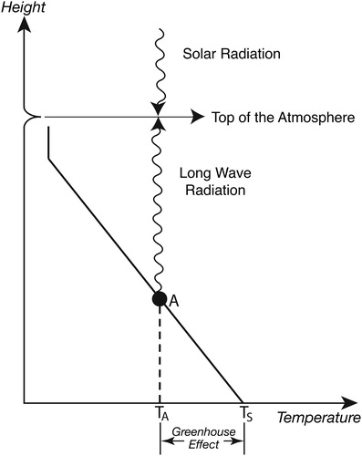
In order to illustrate schematically the thermal structure and the greenhouse effect of the atmosphere, Fig. 1 is constructed. In this figure, the slanted solid line indicates schematically the idealised, vertical temperature profile of the troposphere, where temperature decreases almost linearly with height. The vertical line segment above the slanted line illustrates schematically the almost isothermal lower stratosphere. The dot A in the middle troposphere indicates the effective emission centre of the outgoing terrestrial radiation from the top of the atmosphere. As noted above, its temperature (T_A) is –18.7 °C, which may be compared with +14.5 °C, that is, the global mean temperature of the Earth’s surface (T_S). The latter is warmer than the former by ∼33 °C as noted already, indicating the magnitude of the greenhouse effect of the atmosphere. Using Fig. 1, I would like to explain why the atmosphere exerts such large warming effect upon Earth’s surface.

Fig. 1. Schematic diagram that illustrates the greenhouse effect of the atmosphere. The slanted solid line indicates schematically the vertical temperature profile of the troposphere. The vertical line segment at the top of the slanted line indicates schematically the almost isothermal temperature profile of the stratosphere. The dot A (●) on the slanted line indicates the average height of the layer of emission for the outgoing terrestrial, longwave radiation from the top of the atmosphere. The difference between the global mean surface temperature (T_S) and the temperature of the planetary emission (T_A) indicates the greenhouse effect of the atmosphere.

Radiative transfer in the atmosphere obeys Kirchhoff’s law. This law requires that, for a given wave length, the absorptivity of a substance is equal to its emissivity, which is defined as the ratio of the actual emission to the theoretical emission from a blackbody. Because Earth’s surface behaves almost as a blackbody, it has an absorptivity that is close to one, absorbing almost completely the downward flux of longwave and shortwave radiation that reach Earth surface. In keeping with Kirkhoff’s law, it emits an upward flux of longwave radiation almost as a blackbody would, according to the Stefan–Boltzmann law of blackbody radiation. As this upward flux penetrates into the atmosphere, it is depleted due to the absorption by greenhouse gases such as water vapour, carbon dioxide, nitrous oxide, and methane, but it is also accreted due to the emission from these gases. The net upward flux decreases or increases with height, depending upon whether the depletion is larger than accretion or vice versa.

Although greenhouse gases are minor constituents of the atmosphere, they, as a whole, absorb a major fraction of the upward flux of longwave radiation emitted by the Earth’s surface. On the other hand, the atmosphere emits the upward flux of longwave radiation, partially compensating for the depletion of the upward flux due to the absorption as described above. Since Kirkhoff’s law requires the absorptivity of the atmosphere to be equal to its emissivity at a given wave length, the absorption of the upward flux emitted by the relatively warm Earth’s surface is substantially larger than the emission of the upward flux by the relatively cold atmosphere. For this reason, the emission centre of the outgoing radiation is located in the mid troposphere that is colder than Earth’s surface by ∼33 °C as pointed out already. In short, the atmosphere has greenhouse effect that reduces substantially the upward flux of longwave radiation emitted by the Earth’s surface before it reaches the top of the atmosphere, helping to maintain the warm climate at Earth’s surface.

3. Mechanism of global warming

So far, I have explained why the atmosphere has a so-called greenhouse effect that reduces substantially the upward flux of longwave radiation emitted by Earth’s surface. Here, I shall explain why temperature increases not only at the surface but also in the troposphere as the concentration of a greenhouse gas increases in the atmosphere.

If a greenhouse gas such as carbon dioxide increases in the atmosphere, the infrared opacity of air increases, thereby enhancing the absorption of longwave radiation in the atmosphere. Thus, the absorption of the upward flux from the lower layer of the atmosphere increases more than the absorption of the flux from the higher layer due to the difference in the optical thickness of the overlying layer. Consequently, the average height of the layer, from which the outgoing longwave radiation originates, increases as the concentration of greenhouse gas increases in the atmosphere. In short, the more opaque is the atmosphere, the higher is the emission level of the upward flux that reaches the top of the atmosphere. Since the effective emission centre of the outgoing radiation is located in the troposphere, where temperature decreases with increasing height, the temperature of the centre decreases as it moves upward, thereby reducing the outgoing longwave radiation from the top of the atmosphere.

The physical processes involved in the response of the outgoing, upward flux of longwave radiation to increasing greenhouse gases are illustrated in Fig. 2. In this figure, the slanted solid line indicates schematically the vertical temperature profile in the troposphere, where temperature decreases almost linearly with height. Dot A on the slanted line indicates the effective emission centre for the outgoing longwave radiation from the top of the atmosphere. As indicated by the arrow that originates from the dot A, the effective emission centre moves upward in response to the increase in the concentration of greenhouse gas, as explained above. Thus, the temperature of the centre decreases, reducing the outgoing longwave radiation from the top of the atmosphere.

Fig. 2. Schematic diagram illustrates the upward shift of the dot A (●), which indicates the average height of the layer of the planetary emission for the top-of-the-atmosphere flux of outgoing, longwave radiation, in response to the increase in the concentration of a greenhouse gas in the atmosphere. The diagram also illustrates the downward shift of the dot B (●), which indicates the average height of the layer of emission for the downward flux of the longwave radiation at the Earth surface, in response to the increase in the concentration of a greenhouse gas. Here, the slanted, solid line indicates schematically the vertical temperature profile of the troposphere. The vertical line on the top of slanted line indicate schematically the lower end of almost isothermal stratosphere.

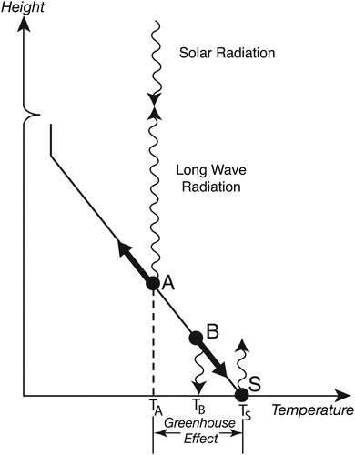
The change in the concentrations of greenhouse gases affects not only the upward flux of the outgoing, longwave radiation from the top of the atmosphere but also the downward flux that reaches the Earth’s surface. If the concentration of greenhouse gas increases in the atmosphere, the infrared opacity of air increases. Thus, the absorption of the downward flux from the higher layer of the atmosphere increases more than the absorption of the flux from the lower layer. Consequently, there is a downward shift of effective level of emission, from which the downward flux originates, as the concentration of greenhouse gas increases in the atmosphere. In short, the more opaque is the atmosphere, the lower is the emission centre of the downward flux that reaches the Earth’s surface. Because temperature increases with decreasing height in the troposphere as indicated by the slanted line in Fig. 1, the temperature at the effective emission level of the downward flux, signified by dot B, also increases as it moves downward, thereby increasing the downward flux of longwave radiation that reaches the Earth’s surface.

The radiative response of the surface-troposphere system to an increase in greenhouse gases can be regarded as the net result of two related processes. The first process involves the increase in the downward flux of longwave radiation that increases the temperature of the Earth’s surface. Over a sufficiently long period of time, the surface returns to the overlying troposphere practically all the radiative energy it receives, with thermal energy being transferred upward through moist and dry convection, longwave radiation, and large-scale circulation in the atmosphere. Thus, temperature increases not only at the Earth’s surface but also in the overlying troposphere.

The second process involves the upward flux of longwave radiation at the top of the atmosphere in response to an increase in atmospheric greenhouse gas concentration. If the amount of greenhouse gases were to increase without allowing the temperature of the surface-troposphere system to change, the upward flux of longwave radiation at the top of the atmosphere would decrease, as explained earlier. To maintain the radiative heat balance of the planet as a whole, the surface-troposphere system warms just enough for the effects of these two processes to balance, such that the top-of-atmosphere flux of outgoing longwave radiation remains unchanged despite the warming. The global scale increase of the overall temperature of the coupled surface-troposphere system is often called global warming.

An important factor that affects the magnitude of global warming is the positive feedback process that involves water vapour. Although it is not shown here, water vapour absorbs and emits strongly over much of the spectral range of terrestrial, longwave radiation and is mainly responsible for the powerful greenhouse effect of the atmosphere. In contrast to long-lived greenhouse gases such as carbon dioxide, water vapour has a short residence time of a few weeks in the atmosphere, where it is added through evaporation from Earth’s surface (e.g. ocean) and is depleted rapidly through condensation and precipitation. Thus, the absolute humidity of air is bounded by saturation, preventing large-scale relative humidity from exceeding 100%. Since the saturation vapour pressure of air increases with increasing temperature according to the Clausius–Clapeyron equation, enhancing the moisture-holding capacity of air, the absolute humidity of air tends to increases with increasing temperature, thereby enhancing the greenhouse effect of the atmosphere. The positive feedback effect between temperature and the greenhouse effect of water vapour is called ‘water vapour feedback’. In short, the water vapour feedback magnifies the global warming that is induced by the increase in the concentration of long-lived greenhouse gas such as CO₂, nitrous oxide, and chlorofluorocarbons (CFCs).

4. Radiative-convective equilibrium

It was toward the end of the 19th century, when Swedish scientist Arrhenius (1896) made the first attempt to estimate the magnitude of temperature change in response to the change in the concentration of carbon dioxide, using one-layer model of the atmosphere coupled with the heat balance model of the Earth’s surface. In his computation, he included not only the water vapour feedback described above but also the snow albedo feedback, that is, the two of the most important positive feedback processes that enhances the sensitivity of climate to thermal forcing. Given the limited information available, it is remarkable that this truly pioneering study was conducted at that time.

Several decades after the publication of Arrhenius’ study, Callendar (1938) made a renewed attempt to estimate the magnitude of surface temperature change in response to the increase in atmospheric carbon dioxide, using absorptivities of carbon dioxide and water vapour that are more realistic than that used by Arrhenius. Callendar, however, employed a very simple method based solely on the radiative energy balance of the Earth’s surface. As explained in the preceding section, the downward flux of longwave radiation increases at the Earth’s surface in response to the increase in the atmospheric concentration of carbon dioxide. In his study, Callendar estimated the magnitude of the increase in surface temperature that yields the increase in the net upward flux of longwave radiation, which is equal to the increase in the downward flux of longwave radiation in response to the increase in the atmospheric concentration of carbon dioxide. His study attracted the attention as it apparently simulated the global warming observed during the several decades around 1900AD.

A few decades after the publication of Callendar’s study, Möller (1963) conducted careful evaluation of the study, using the latest information available at that time. He found that, although the Callendar’s approach yielded surface temperature change of plausible magnitude in the absence of the water vapour feedback, it fails to do so as discussed below, when the feedback is incorporated into the model.

As explained in the preceding section, the absolute humidity of air in the troposphere tends to increases with increasing temperature in the presence of the water vapour feedback, thereby increasing the downward flux of longwave radiation at the Earth’s surface. For this reason, the net upward flux of longwave radiation at the surface hardly increases with increasing temperature in the presence of the water vapour feedback, making it problematic to estimate the change in surface temperature using Callendar’s method. Mӧller speculated that, for reliable estimate of the surface temperature change that satisfies the heat balance requirement, it may be necessary to consider not only the net upward flux of longwave radiation but also the convective heat flux from Earth’s surface to the overlying troposphere. For further discussion of this subject, see chapter 2 of the book ‘Beyond Global Warming’ (Manabe and Broccoli, 2019) to be published by Princeton University Press.

In the middle of 1960’s, Manabe and Wetherald (1967) addressed this issue, using one-dimensional, radiative-convective model, in which the heat balance of the atmosphere and that of the Earth’s surface are maintained through the close interaction between radiative and convective heat transfer. Using the model, they obtained the vertical temperature profile of the atmosphere in radiative-convective equilibrium not only for the normal concentration of carbon dioxide, that is, 300 ppm by volume, but also for two other concentrations, that is, 150 ppmv and 600 ppmv.

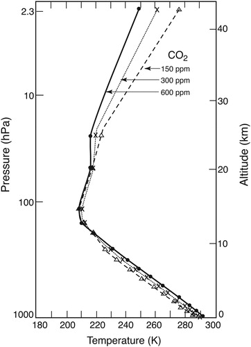
Figure 3 illustrates vertical temperature profiles of the coupled atmosphere-earth surface system in radiative-convective equilibrium, which is obtained for the three concentrations identified above. As explained already in the preceding section, temperature increases not only at Earth’s surface but also in the troposphere as the concentration of atmospheric carbon dioxide doubles from 150 ppm to 300 ppm and 300 ppm to 600 ppm. The magnitude of the warming is 2.3 °C in both cases and is practically identical to each other. Since the absorptivity of carbon dioxide is approximately proportional to the logarithm of its concentration, it is expected that the greenhouse effect of the atmosphere changes in proportion of the logarithm of the amount of carbon dioxide in the atmosphere. This explains the reason why the magnitude of the warming due to the doubling of atmospheric carbon dioxide from 150 ppm to 300 ppm is similar to the warming due to the doubling from 300 ppm to 600 ppm even though the magnitude of the change in the concentration of carbon dioxide is much smaller in the former than in the latter.

Fig. 3. Vertical profiles of temperature in radiative-convective equilibrium. Dashed, dotted and solid lines illustrate the vertical profiles obtained for the three different atmospheric concentrations of carbon dioxide, that is, 150 ppm (part per million), 300 ppm, and 600 ppm by volume, respectively. Temperature is indicated at the bottom of the figure. Pressure (hp) and approximate height (km) are indicated on the left and right of the figure, respectively. From Manabe and Wetherald (1967).

To evaluate quantitatively the influence of the water vapour feedback upon the simulated warming, they conducted another set of runs in which the feedback was disabled. In these runs, the distribution of absolute humidity was prescribed to remain constant rather than being adjusted to maintain a constant relative humidity. From the differences among the three states of radiative-convective equilibrium thus obtained, Manabe and Wetherald estimated the magnitude of the equilibrium response of surface temperature in the absence of water vapour feedback. They found that surface temperature increases by approximately 1.3 °C in response to the doubling of atmospheric CO₂ concentration not only from 150 ppm to 300 ppm but also from 300 ppm to 600 ppm. It is much smaller than 2.3 °C that we got in the presence of water vapour feedback. The results from these experiments indicate that the water vapour exerts strong a positive feedback effect that magnifies the surface temperature change by a factor of ∼1.8.

In sharp contrast to the Earth’s surface and troposphere, where temperature increases in response to a doubling of the atmospheric CO₂ concentration, cooling occurs in the stratosphere as indicated in Fig. 3. Because of the absence of convective heating, the heat balance of the stratosphere is maintained between the heating due to the absorption of solar radiation by ozone and the net cooling due to the emission and absorption of longwave radiation mainly by carbon dioxide. If the atmospheric CO₂ concentration doubles, for example, the longwave cooling intensifies and temperature in the stratosphere equilibrates at a lower value. This is the main reason why the stratospheric cooling occurs in the CO₂-doubling experiment as shown in Fig. 3.

According to analysis of data obtained from satellite microwave sounding and radio-sonde measurements (Karl et al., 2006), the global mean temperature has decreased at the rate of ∼0.4 °C per decade in the lower stratosphere, and increased at the rate of ∼0.2 °C per decade in the lower troposphere, during the last half century. The reversal of temperature trends between the stratosphere and troposphere appears to be in agreement with the result obtained from the radiative-convective model described here. It is likely, however, that the observed cooling in the lower stratosphere is attributable not only to the increase in the concentration of carbon dioxide but also to the reduction of ozone in the stratosphere as pointed out, for example, by Ramaswamy (2006).

5. Coupled atmosphere-ocean-land model

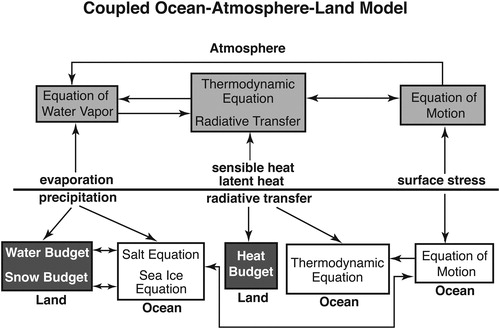
The one-dimensional, radiative-convective model introduced above was developed as an important step towards the development of a three-dimensional, general circulation model of the atmosphere, which evolved into a coupled model of the atmosphere-ocean-land system to be called hereafter ‘coupled model’ for ease of identification. The performance of the initial version of the coupled model was described in a paper published by Manabe and Bryan (1969). As shown in the box diagram in Fig. 4, the coupled model consists of three major components, which are the general circulation model of the atmosphere, that of ocean, and the simple, heat- and water- balance model of continental surface. For computational economy, parameterisation of various subgrid scale processes (e.g. moist convection, cloud formation, heat- and water-budget at continental surface) were made as simple as possible without losing its essential function. Although the initial version of the coupled model was constructed in the late 1960’s, it took two more decades before the coupled model with realistic geography became ready for the global warming experiment described below. For the description of this version of the coupled model and design of the numerical experiments performed, see Manabe et al. (1991).

Fig. 4. Diagram that depicts schematically the structure of the coupled atmosphere-ocean-land model.

Starting in 1989, we published a series of papers (Stouffer et al. 1989; Manabe et al. 1991, 1992) that describes the results from a climate prediction experiment conducted in the late 1980’s. In the experiment, the coupled model was forced by the atmospheric concentration of carbon dioxide that increases at the rate of 1% per year, compounded. This rate is roughly equivalent to the rate of increase in the radiative forcing due to the increase of all greenhouse gases since the late 1980’s (see Schimmel, 1995), not including ozone change.

Here, I describe briefly our recent attempt (Stouffer and Manabe, 2017) to compare the distribution of the surface temperature predictions made more than 25 years ago with observations made during the last half century. An important caveat to keep in mind is that the model forcing used in the study involved the increase in the equivalent CO₂ concentration of greenhouse gases. Changes in other forcing agents such as man-made and volcanic aerosols, and insolation were ignored. The forcing difference between solely CO₂ versus all the known radiative forcing agents are likely to cause differences in the pattern and magnitude of the change shown here. This causes problems in comparing models to observations and makes the comparisons qualitative in nature. It is one of the reasons why we focus our attention on the geographical distribution of surface temperature change rather than the magnitude of change in this study.

Figure 5a illustrates the geographical distribution of the predicted change in surface air temperature by the ∼70th year of the global warming experiment, when the atmospheric concentration of carbon dioxide doubles in the experiment. It may be compared with Fig. 5b, which illustrates the distribution of the difference in observed surface temperature between the recent 25-year period 1991–2015 and the 30-year reference period 1961–1990. The difference may be regarded as an indicator of the local temperature trends during the last half century when the multi-decadal rate of global warming is the most pronounced. In order to facilitate comparison between the geographical patterns of predicted and observed surface temperature changes that are different by a factor of ∼5, colours are chosen such that the values at the various colour thresholds in Fig. 5a are five times as large as those in Fig. 5b, highlighting the warming pattern.

Fig. 5. Geographical distribution of the change in surface air temperature. (a) Change in the coupled model realised by the ∼70th year (the average between the 60th and 80th year) of the global warming experiment, when the atmospheric concentration of carbon dioxide doubles. Here, surface air temperature is obtained from the atmospheric model level closest to Earth’s surface (∼75 m). (b) Observed change from the 30-year base period around 1975 (1961–1990) to the 25-year period around 2002 (1991–2015). The map is obtained using the historical surface temperature data set HadCRUTS4 described by Morice et al. (2012). Note that, in the Southern Ocean poleward of 60°S, the observed change is not shown because data are hardly available in winter. From Stouffer and Manabe (2017).

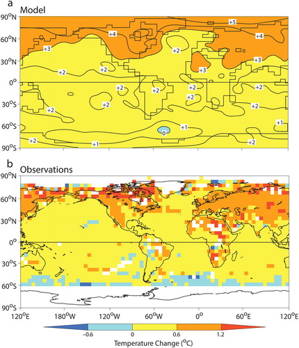
Comparing the pattern of predicted and observed change, it is notable that surface temperature increases almost everywhere with land areas warm faster than adjacent ocean areas in both model and observation. As explained already, the downward flux of longwave radiation increases at the Earth’s surface as the concentration of greenhouse gas increases in the atmosphere, thereby increasing the surface temperature. The magnitude of the warming is larger over continent than over ocean, where much of net incoming radiation is used as the latent heat of evaporation, reducing the warming. Inspecting Fig. 5a, one notes that the warming is a minimum in the northern North Atlantic, though this is not so pronounced in the observation (Fig. 5b). This minimum is attributable not only to deep convective mixing of heat but also to the weakening of the Atlantic meridional overturning circulation that carries warm water toward the northern North Atlantic.

Figure 5 also indicates that, in both the model and the observation, the warming tends to increase with increasing latitudes in the Northern Hemisphere. In sharp contrast, temperature change is small in the Antarctic Ocean in both the model result and observation. If the observed trend of little or no warming continues in the Southern Ocean, it will confirm this surprising early model finding.

To discuss the reason why the surface temperature does not change substantially in the Southern Ocean of the model, we present Fig. 6 that illustrates the latitude-depth profile of zonally averaged, oceanic temperature change realised by the 70th year of the experiment, when the concentration of carbon dioxide doubles in the atmosphere. This figure reveals that the positive temperature anomaly penetrates deeply not only near the Antarctic coast around 75°S but also in the circumpolar ocean around 60°S. As pointed out by Manabe et al. (1991), this is attributable to the deep convection that mixes heat deeply, increasing greatly the effective thermal inertia of ocean. Consequently, the magnitude of the warming is small at the surface of the circumpolar ocean as indicated in Fig. 5a.

Fig. 6. Zonally averaged temperature change (°C) for the entire ocean of the coupled model realised by the ∼70th year of the global warming experiment, when the atmospheric concentration of carbon dioxide doubles. From Stouffer et al. (1989).

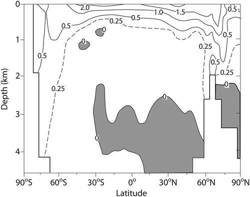
In the circumpolar ocean of the Southern Hemisphere zonally connected around latitude circle, intense westerlies predominate in the atmosphere, driving the deep overturning circulation as Gill and Bryan (1971) explained. In the upwelling segment of the overturning circulation, located around 60°S, sea ice forms in winter beneath frigid air and grows rapidly, producing patches of saline, dense water at oceanic surface through brine release. Thus, they sink deeply, yielding deep convection. Meanwhile, the upwelling of deep water prevents the continuous accumulation of dense saline water in the deep layer of the ocean, helping to sustain deep convection. In short, the upwelling of deep water is critically important for sustaining deep convection in the Southern Ocean.

The existence of the deep overturning circulation in the Southern Ocean was questioned by Danabasoglu et al. (1994). However, it is quite likely to exist, playing critically important role in the heat budget in the Southern Ocean. For further discussion of this subject, see chapter 8F of the book ‘Beyond Global Warming’ (Manabe and Broccoli, 2019) to be published soon by Princeton University Press.

In summary, the geographical patterns of the predicted and observed surface temperature change are very similar to each other. This is quite surprising, when one realises that the distribution of the thermal forcing of the model does not include the effect of aerosols and is likely to be substantially different from that of the actual forcing. Nevertheless, the similarity between the predicted and observed patterns suggests that the geographical pattern of surface temperature change may not depend critically upon that of thermal forcing. It also suggests that the model contains the key physical processes that control the geographical pattern of global warming at the Earth’s surface.

6. Change in water availability

Global warming involves changes not only in temperature but also in the rate of evaporation and that of precipitation. If a greenhouse gas such as water vapour and carbon dioxide increases in the atmosphere, the downward flux of longwave radiation increases at the Earth’s surface, thereby increasing the surface temperature as explained in Section 3. Since the saturation vapour pressure of air at a wet surface (e.g. ocean) increases with increasing surface temperature, it is expected that the rate of evaporation from the Earth’s surface also increases so long as the relative humidity of the overlying atmosphere does not change systematically. Given sufficient time, global-scale increase in the rate of evaporation in turn results in corresponding increase in the rate of precipitation, increasing the strength of the global water cycle.

As Manabe and Wetherald (1975, 1985) and Held and Soden (2006) pointed out, global warming affects not only the global mean rates of precipitation and evaporation but also their geographical distributions due mainly to the change in the rate of horizontal transport of water vapour by large-scale circulation in the atmosphere. When temperature increases in the troposphere in response to the increase in the concentration of greenhouse gas, it is expected that the horizontal transport of water vapour by large-scale circulation also increases in the troposphere, because the absolute humidity of air tends to increase with increasing temperature, keeping relative humidity unchanged as discussed already in Section 3. This is the main reason why the distribution of precipitation changes differently from that of evaporation as global warming proceeds, affecting substantially the distribution of the water availability such as the rate of river discharge and soil moisture at continental surface.

Here, I shall discuss how the distributions of precipitation and evaporation are likely to change in response to the increase in the atmospheric concentration of carbon dioxide, thereby affecting river discharge and soil wetness at continental surface. It is based upon the analysis of the numerical experiments described by Wetherald and Manabe (2002) and Manabe et al. (2004a, 2004b). The structure of the model used is similar to the coupled model described in the preceding section. In order to obtain distribution of precipitation that is realistic enough for these experiments, however, the computational resolution of the model was doubled, reducing the interval between finite difference grid points by a factor of two from ∼500 km to ∼250 km.

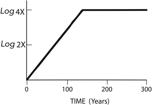
In the numerical experiment presented here, the atmospheric concentration of carbon dioxide increases at the compounded rate of 1% per year until it quadruples and remains unchanged as shown schematically in Fig. 7. By comparing the state at the end of the experiment with the initial state of the model, we evaluated how the distributions of hydrologic variables change in response to quadrupling of the atmospheric concentration of carbon dioxide. Although similar numerical experiment was performed for CO₂-doubling, the result is not presented here because the geographical pattern of the hydrologic changes obtained from the two experiments are similar to each other, though their magnitude differs by a factor of ∼2.

Fig. 7. Time series of atmospheric CO₂ concentration (in logarithmic scale). Here, X and 4X denote 300 ppm by volume and 1200 ppm by volume, respectively.

Figure 8 shows the latitudinal distribution of zonally averaged, annual mean rate of evaporation and that of precipitation simulated by the model. Although both precipitation and evaporation are lager in low latitudes than in high latitudes, their profiles are different. For example, the zonal mean rate of precipitation is larger than that of evaporation near the equator and from middle to high latitudes, whereas the reverse is the case in the subtropics. The difference between the two profiles is attributable mainly to the change in the meridional transport of water vapour by atmospheric circulation.

Fig. 8. Latitudinal profiles of annual mean rate of evaporation (dashed line) and that of precipitation (solid line), zonally averaged over latitude circle. They are obtained from the control run, in which CO₂ concentration is held fixed at the standard value (i.e. 300 ppm by volume). From Wetherald and Manabe (2002).

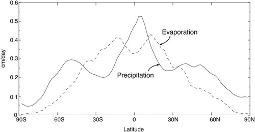
An important factor that controls the latitudinal profiles of precipitation and evaporation at low latitudes is Hadley Circulation with rising motion near the equator and sinking motion in the subtropics. In the near-surface layer of the atmosphere, trade-winds carry moisture-rich air from the subtropics toward the tropical convergence zone, where intense upward motion predominates and precipitation is at a maximum. In the subtropics, on the other hand, air sinks in broad zonal belt. Because of adiabatic compression of this sinking air, relative humidity is low, enhancing evaporation from the Earth’s surface. Thus, evaporation is at a maximum in the subtropics.

At middle latitudes, where extratropical cyclones are frequent, precipitation is at a maximum. These cyclones carry warm, humid air poleward and cold, dry air equatorward, yielding the net transport of water vapour from the subtropics toward the middle and high latitudes. Thus, atmospheric circulation transports water vapour from the subtropics, where evaporation exceeds precipitation, to middle and high latitudes, where precipitation exceeds evaporation.

In order to show how the latitudinal profile of precipitation and that of evaporation changes in response to the quadrupling of CO₂ concentration in the atmosphere, Fig. 9 is constructed. As this figure shows in magnified scale, the zonal mean rate of evaporation increases at almost all latitudes. The magnitude of the increase is large in the tropics and decreases poleward, becoming small in high latitudes. Because the vapour pressure of air in contact with a wet surface (e.g. oceanic surface) increases with increasing surface temperature according to Clausius–Clapeyron equation, the vertical gradient of vapour pressure above the surface also increases as long as the relative humidity of overlying air does not change systematically. This is the main reason why the increase in the rate of evaporation is largest at low latitudes, where the surface temperature is highest, and decreases with increasing latitudes.

Fig. 9. Latitudinal profiles of zonally averaged change in the annual mean rates of evaporation and precipitation in response to quadrupling of atmospheric concentration of carbon dioxide.

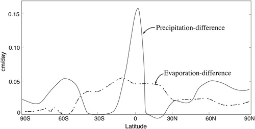
In response to the increase in evaporation described above, the zonal mean rate of precipitation also increases at most latitudes as shown in Fig. 8. The latitudinal distribution of the change in the rate of precipitation, however, is quite different from that of evaporation. As shown on a magnified scale in Fig. 9, the rate of precipitation increases much more than that of evaporation in the tropics and in middle and high latitudes, whereas the reverse is the case in subtropics. These changes are attributable mainly to the increase in the export of moisture from the subtropics toward other latitudes.

When temperature increases in the troposphere owing to global warming, absolute humidity also increases, keeping relative humidity almost unchanged, as discussed earlier. The increase in absolute humidity in turn results in the increase in the transport of tropospheric water vapour. For example, the poleward transport of water vapour by extra-tropical cyclones increases, thereby increasing the transport of moisture from the subtropics toward middle and high latitudes. Thus, precipitation increases more than evaporation poleward of 45° in both hemispheres as shown in Fig. 9. Meanwhile, the equator-ward transport of water vapour by trade winds also increases, increasing the supply of moisture toward the tropical rainbelt, where precipitation increases much more than evaporation. On the other hand, because of the increase in the export of moisture toward both high and low latitudes, precipitation hardly changes in the subtropics despite increased supply of moisture through evaporation from the Earth’s surface to the atmosphere. Held and Soden (2006) found similar hydrologic responses in their analysis of the climate change experiments used for the Fourth Assessment Report of the Intergovernmental Panel on Climate Change.

Because of the changes in rates of precipitation and evaporation described above, water availability also changes at continental surface. For example, the rate of river discharge increases in many regions in middle and high latitudes and in the tropics, where the zonal mean rate of precipitation increases more than evaporation. In contrast, over many arid and semi-arid regions in the subtropics, soil moisture often decreases substantially. Since the downward flux of longwave radiation increases at the Earth’s surface in response to the increase in the concentration of greenhouse gases, the thermal energy available for evaporation increases at Earth’s surface. On the other hand, precipitation hardly increases or decreases in much of the subtropics owing to the increased export of water vapour toward both high and low latitudes. For these reasons, it is expected that soil moisture decreases substantially over many arid and semi-arid regions in the subtropics. In the remainder of this section, we will describe how geographical distribution of soil moisture changes over continents as a consequence of global warming.

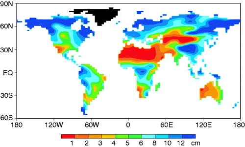
A meaningful and direct comparison of modelled soil moisture with observations is not possible, because of difficulties in defining the plant-available water-holding capacity of the soil, and because of the extreme heterogeneity of soil moisture, soil properties and vegetation rooting characteristics. Nevertheless, soil moisture in this model is an excellent indicator of soil wetness and associated biome. Fig. 10 illustrate the distribution of annual mean soil moisture simulated by the model. The model reproduces reasonably well very broad scale features of soil wetness. For example, the regions of very low soil moisture simulated by the model approximately correspond with the major arid regions of the world: Gobi and Great Indian Desert of Eurasia, North American deserts, Australian deserts, the Patagonian Desert of South America, and the Sahara and Kalahari deserts of Africa. Furthermore, the model places reasonably well the semi-arid regions (green in Fig. 10) in Africa, Australia, and Eurasia. Although semi-arid, western plain of North America is simulated by the model, it extends eastward too far particularly in the southern US, where precipitation is underestimated substantially. On the other hand, soil moisture is large in Siberia and Canada located in high northern latitudes, where precipitation exceeds slow evaporation. As expected, soil moisture is also large in heavily precipitating regions of tropics in South America, Southeast Asia and Africa. In summary, the model places reasonably well the locations of arid, semi-arid and wet regions of the world.

Fig. 10. Geographical distribution of annual mean soil moisture (cm) obtained from the control run. Here, soil moisture is defined as the difference between the total amount and the wilting point of water in the root zone of soil. From Wetherald and Manabe (2002).

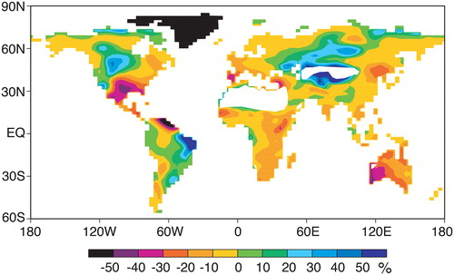
Figure 11 illustrates, in term of the percentage of the value obtained from the control experiment with the standard CO₂ concentration, the geographical distribution of the change in annual mean soil moisture in response to the quadrupling of atmospheric concentration of carbon dioxide. Inspecting the figure, one can see that the percentage reduction is relatively large in many arid and semi-arid regions of the world such as western and southern part of Australia, southern part of Africa, southern Europe, northeastern region of China, and southwestern portion of North America. Although the percentage reduction is also large in the southeastern US, the result should be regarded with caution, because simulated soil moisture is too small in the region as indicated by green colour in Fig. 10.

Fig. 11. Geographical distributions of the percentage change in annual mean soil moisture in response to quadrupling in the atmospheric concentration of carbon dioxide. Here, the percentage change is defined as the percentage of the time mean soil moisture obtained from the control experiment. It is not shown in the extremely arid regions such as Sahara and Central Asia, where soil moisture is less than 1 cm as shown in Fig. 10. In these regions, soil moisture is so small that its percentage change is indefinite. From Manabe et al. (2004b).

Why does soil moisture decreases in many relatively arid regions of the world? As we have discussed previously, the downward flux of longwave radiation increases owing to the increase in the concentration of greenhouse gases, thereby increasing the total radiative energy that is potentially available for evaporation. On the other hand, the magnitude of the change in precipitation is usually small in these regions. In order to maintain the water balance of the continental surface, it is therefore necessary to reduce evaporation as a fraction of potential evaporation. Because the ratio of evaporation to potential evaporation decreases as soil dries, a reduction in soil moisture reduces the fraction of the radiative energy used for evaporation. This is the main reason why soil moisture decreases in many arid and semi-arid regions of the world.

In many relatively arid regions of the world, soil moisture is small partly because water vapour is exported outward by atmospheric circulation as it is in many regions in the subtropics. Because absolute humidity of air usually increases with increasing temperature as explained already, it is expected that the rate of export is likely to increase as global warming proceeds, reducing the amount of water vapour available for precipitation in these regions. This is another reason why soil moisture decreases in many relatively arid regions of the world.

If greenhouse gas continues to increase, the reduction of soil moisture in many arid and semi-arid regions of the world is going to be increasingly noticeable during the 21st century as explained in the preceding paragraphs. Unfortunately, river discharge in many of these regions is likely to decrease as global warming proceeds (Milly et al., 2008). It is therefore likely that the shortage of water in these regions could become very acute during the next few centuries. In contrast, an excessive amount of water is likely to be available through river discharge in many water-rich regions in high northern latitudes and in heavily precipitating regions of tropics. Thus, the frequency of floods is likely to increase markedly as Milly et al. (2002) found in a global warming experiment. The implied amplification of existing differences in water availability between water-poor and water-rich regions could become a very challenging issue for mankind.

7. Concluding remarks

From the 1960’s to the late 1980’s, when we developed the models used for the studies presented here, computers were much slower than those used currently. This is one of the important reasons why the parameterisations of various subgrid scale processes were made as simple as possible. Nevertheless, it was encouraging that these models successfully simulated many salient features of climate. It is also encouraging that a general circulation model of the coupled atmosphere-ocean-land system, constructed about 30 years ago, successfully simulated the geographical pattern of the surface temperature change that has been observed during the last several decades as shown in Fig. 5 shown in Section 5.

Owing partly to the simplicity of parameterisations and low resolution, the computational requirement of the coupled atmosphere-ocean-land model introduced here, is much smaller than the climate models that are currently used for predicting climate change. This is one of the reasons why it has been possible to conduct many numerical experiments, changing one factor at a time, using the model as a virtual laboratory for examining the inner workings of the climate system. In fact, the simplicity of parameterisation has facilitated greatly the diagnostic analysis of the result obtained. For these reasons, relatively simple climate models such as the coupled atmosphere-ocean-land model introduced here have been and are likely to be very powerful tools for exploring climatic change of not only the industrial present but also the geological past.

Acknowledgements

It is a great honour to be chosen by the Royal Swedish Academy of Sciences to receive the Crafoord Prize established through the generosity and farsightedness of Mr. and Mrs. Crafoord. It is likewise a great pleasure to give a talk on global warming, that is, the subject that I have enjoyed exploring throughout my career. On this occasion, I would like to thank Joseph Smagorinsky, the inaugural director of Geophysical Fluid Dynamics Laboratory of National Oceanic and Atmospheric Administration, USA, with whom I collaborated for the initial development of the three-dimensional climate model used for the study presented here. I am receiving this award for the fruits of close collaboration among the staff members of the laboratory. It has been a great privilege and pleasure to work with them.

Disclosure statement

No potential conflict of interest was reported by the authors.

References

- Arrhenius, S. 1896. On the influence of carbonic Acid in the air upon the temperature of the ground. Phil. Mag. Ser. 5, 237–276.
- Callendar, G. S. 1938. The artificial production of carbon dioxide and its influence on temperature. Qjr. Meteorol. Soc. 64, 223–240.
- Danabasoglu, G., McWilliams, J. C. and Gent, P. R. 1994. The role of mesoscale tracer transports in the global circulation. Science 264, 1123–1126. doi: 10.1126/science.264.5162.1123
- Gill, A. E. and Bryan, K. 1971. Effect of geometry on the circulation of a three-dimensional, southern-hemisphere ocean model. Deep Sea Res. 18, 685–721.
- Held, I. M. and Soden, B. J. 2006. Robust response of the hydrologic cycle to global warming. J. Clim. 19, 5686–5699. doi: 10.1175/JCLI3990.1
- Karl, T.R., Hassol, S.J., Miller, C.D. and Murray W.L. (eds.). 2006. Temperature Trends in the Lower Atmosphere: Steps for Understanding and Reconciling Differences. A Report by the Climate Change Science Program and Subcommittee on Global Change Research, Washington, DC, 180 pp.
- Loeb, N. G. et al. 2009. Towards original closure of the Earth's top-of-atmosphere radiation budget. J. Clim. 22, 748–766.
- Manabe, S. and Bryan, K. 1969. Climate calculation with a combined ocean-atmosphere model. J. Atmos. Sci. 26, 786–789. doi: 10.1175/1520-0469(1969)026<0786:CCWACO>2.0.CO;2
- Manabe, S. and Broccoli, A. J. 2019. Beyond Global Warming: How Numerical Models Revealed the Secrets of Climate Change. Princeton, NJ: Princeton University Press.
- Manabe, S. and Wetherald, R. T. 1967. Thermal equilibrium of the atmosphere with a given distribution of relative humidity. J. Atmos. Sci. 24, 241–259. doi: 10.1175/1520-0469(1967)024<0241:TEOTAW>2.0.CO;2
- Manabe, S. and Wetherald, R. T. 1975. The effect of doubling CO2 concentration on the climate of a general circulation model. J. Atmos. Sci. 32, 3–15. doi: 10.1175/1520-0469(1975)032<0003:TEODTC>2.0.CO;2
- Manabe, S. and Wetherald, R. T. 1985. CO2 and Hydrology. Advances in Geophysics. 28. Issues in Atmospheric and Oceanic Modeling. Part A, Climate Dynamics (ed. S. Manabe). New York, NY: Academic Press, 131–157.
- Manabe, S., Stouffer, R. J., Spelman, M. J. and Bryan, K. 1991. Transient response of a coupled ocean atmosphere model to gradual changes of atmospheric CO2. Part I: Annual mean response. J. Clim. 4, 785–818. doi: 10.1175/1520-0442(1991)004<0785:TROACO>2.0.CO;2
- Manabe, S., Spelman, M. J. and Stouffer, R. J. 1992. Transient response of a coupled ocean atmosphere model to gradual changes of atmospheric CO2. Part II: Seasonal response. J. Clim. 5, 105–126. doi: 10.1175/1520-0442(1992)005<0105:TROACO>2.0.CO;2
- Manabe, S., Wetherald, R. T., Milly, P. C. D., Delworth, T. L. and Stouffer, R. J. 2004a. Century-scale change in water availability: CO2-quadrupling experiment. Clim. Change 64, 59–76. doi: 10.1023/B:CLIM.0000024674.37725.ca
- Manabe, S., Milly, P. C. D. and Wetherald, R. T. 2004b. Simulated long-term changes in river discharge and soil moisture due to global warming. Hydrol. Sci. J. 49, 625–642.
- Milly, P. C. D., Wetherald, R. T., Dunne, K. A. and Delworth, T. L. 2002. Increasing risk of great floods in a changing climate. Nature 415, 514–517. doi: 10.1038/415514a
- Milly, P. C. D., Betancourt, J., Falkenmark, M., Hirsch, R. M., Kundzewicz, Z. K. and co-authors. 2008. Climate change. Stationarity is dead: whither water management? Science 319, 573–574. doi: 10.1126/science.1151915
- Möller, F. 1963. On the influence of changes in the CO2 concentration in air on the radiation balance of earth’s surface and climate. J. Geophys. Res. 68, 3877–3886. doi: 10.1029/JZ068i013p03877
- Morice, C. P., Kennedy, J. J., Raynor, N. A. and Jones, P. D. 2012. Quantifying uncertainties in global and regional temperature change using an ensemble of observational estimates: The HadCRUTS4 data set. J. Geophys. Res. 117, D08101.
- Ramaswamy, V. 2006. Anthropogenic and natural influences in the evolution of lower stratospheric cooling. Science 311, 1138–1141. doi: 10.1126/science.1122587
- Schimmel, D. 1995. Climate Change 1995: The Science of Climate Change (eds J.T. Houghton). Cambridge: IPCC, Cambridge University Press, 65–132.
- Stouffer, R. J. and Manabe, S. 2017. An assessment of temperature pattern projection made in 1989. Nature Clim. Change. 7, 163–165. doi: 10.1038/nclimate3224
- Stouffer, R. J., Manabe, S. and Bryan, K. 1989. Interhemispheric asymmetry in climate response to a gradual increase of atmospheric CO2. Nature 342, 660–662. doi: 10.1038/342660a0
- Wetherald, R. T. and Manabe, S. 2002. Simulation of hydrologic changes associated with global warming. J. Geophys. Res. 107, 4379–4393. doi: 10.1029/2001JD001195