
 ?Mathematical formulae have been encoded as MathML and are displayed in this HTML version using MathJax in order to improve their display. Uncheck the box to turn MathJax off. This feature requires Javascript. Click on a formula to zoom.
Abstract
Numerical weather prediction (NWP) models are moving towards km-scale (and smaller) resolutions in order to forecast high-impact weather. As the resolution of NWP models increase the need for high-resolution observations to constrain these models also increases. A major hurdle to the assimilation of dense observations in NWP is the presence of non-negligible observation error correlations (OECs). Despite the difficulty in estimating these error correlations, progress is being made, with centres around the world now explicitly accounting for OECs in a variety of observation types. This paper explores how to make efficient use of this potentially dramatic increase in the amount of data available for assimilation. In an idealised framework it is illustrated that as the length-scales of the OECs increase the scales that the analysis is most sensitive to the observations become smaller. This implies that a denser network of observations is more beneficial with increasing OEC length-scales. However, the computational and storage burden associated with such a dense network may not be feasible. To reduce the amount of data, a compression technique based on retaining the maximum information content of the observations can be used. When the OEC length-scales are large (in comparison to the prior error correlations), the data compression will select observations of the smaller scales for assimilation whilst throwing out the larger scale information. In this case it is shown that there is a discrepancy between the observations with the maximum information and those that minimise the analysis error variances. Experiments are performed using the Ensemble Kalman Filter and the Lorenz-1996 model, comparing different forms of data reduction. It is found that as the OEC length-scales increase the assimilation becomes more sensitive to the choice of data reduction technique.
1. Introduction
In numerical weather prediction (NWP), the assimilation of observations and prior information (commonly referred to as the background) is performed routinely to find the most probable state of the atmosphere represented on the model grid. Data assimilation (DA) has proven to be essential for accurate weather forecasting by providing the initial conditions for NWP (Rabier et al., Citation2000; Rawlins et al., Citation2007).
With increasing computer power, the resolution of NWP models are increasing with the aim of improving the accuracy of high-impact small-scale events. In order to constrain these models there is an increasing need for higher spatial and temporal resolution observations. These observational needs may potentially be met by the next generation of geostationary satellites (e.g. Advanced Himawari Imager onboard Himawari-8, The Infrared Sounder onboard MTG-S) and phased array weather Radars (Miyoshi et al., Citation2016). However, there are currently many factors limiting the use of the large datasets produced by these observations. These include issues with data storage, computational time and complications caused by correlated errors, which are difficult to estimate and complicate the DA algorithms (Liu and Rabier, Citation2003). To address these issues observations are commonly thinned (both spatially, temporally and spectrally) (e.g. Rabier et al., Citation2002; Dando et al., Citation2007; Migliorini, Citation2015; Fowler, 2017) and ‘super-obbed’ (Berger and Forsythe, Citation2004; van Leeuwen, Citation2015). Variances are also commonly inflated (Hilton et al., Citation2009) to reduce the impact of the sub-optimal use of observations that are known to have correlated errors not represented during the assimilation.
The main hurdle to the use of observation error correlations (OECs) in DA is the difficulty in estimating them as they are often attributed to uncertainty in the comparison of the observations to the model variables, known as representation error, rather than instrument noise (see Janjic et al., Citation2017 and references there in). As such they can be state and model dependent (Waller et al., Citation2014) and are predominantly found in observation types with complex observation operators (such as satellite radiances Bormann and Bauer, Citation2010; Stewart et al., Citation2014; Waller et al., Citation2016a; Bormann et al., Citation2016; Campbell et al., Citation2017), observation types measuring features with natural length- and time-scales that are different to those resolved by the model (e.g. Doppler radial winds Waller et al., Citation2016b), and high level observation products which go through a large amount of preprocessing (e.g. atmospheric motion vectors (AMVs) derived from satellite radiances Bormann et al., Citation2003; Cordoba et al., Citation2017). However, progress is being made in estimating and allowing for the presence of correlated observation errors in DA operationally (e.g. Weston et al. Citation2014; Bormann et al., Citation2016; Campbell et al., Citation2017), potentially facilitating the assimilation of much denser observations. This barrier to the use of dense observations is therefore reducing, however issues with computational effort still remain.
Instead of regular thinning, the compression of the data may allow for much of the information within the observations to be retained while still reducing the computational cost of assimilating the data. Data compression, via principle component analysis, has previously been suggested and tested on hyper-spectral satellite instruments such as AIRS and IASI (Collard et al., Citation2010). It is generally found that the atmospheric signal contained in the original spectrum of a few thousand radiances can be represented by about 200 globally generated principal components (Goldberg et al., Citation2003). However, the observations that provide the greatest constraint for estimating the initial state depend not only on the observations and their uncertainty but also on the information already provided by the prior. This is acknowledged in channel selection methods, which use metrics such as mutual information and degrees of freedom for signal to choose a subset of the most informative channels for selection based on a typical prior error covariance matrix (e.g. Rabier et al. Citation2002; Migliorini, Citation2015; Fowler, 2017). However, the prior error covariance matrix can be highly flow dependent, as such the information content of the observations will also be flow dependent. This flow-dependency is naturally represented by DA methods based on the Ensemble Kalman Filter.
Other methods for intelligent network design include adaptive methods such as targeted observations. These methods depend not only on the observation and prior uncertainty but also on the error growth in the forecast model. This allows regions to be identified where additional observations would reduce the forecast error. A variety of techniques have been developed to measure the forecast sensitivity to perturbations to the initial conditions, including those based on the forecast adjoint model, singular vectors and ensemble techniques (see review by Majumdar, Citation2016).
For high-resolution forecasting, which is the focus of this paper, nested grids are often used with lead-times of h. For example, the UK Met Office runs a nested grid over the UK at a resolution of 1.5 km concentrating on precipitation forecasts out to 6 h (Li et al., Citation2018). Rapid up-date forecasting systems are also under development at centres such as RIKEN-Center for Computational Science, that perform DA at resolutions up to 100 m on a local domain in order to produce 30 min forecasts (Miyoshi et al., Citation2016). At these shorter lead times, the influence of the observation on the analysis, rather than the forecast, becomes more insightful in defining an optimal data compression strategy.
This work demonstrates how spatially correlated observation errors affect the influence of the observations on the analysis. In turn this is used to explain how spatially correlated observation errors affect the use of data reduction techniques within the ensemble Kalman Filter.
It is known that observations with correlated errors provide more information about small-scale features than observations with uncorrelated error (Seaman, Citation1977; Rainwater et al., Citation2015; Fowler et al., Citation2018). As such the use of dense observations is shown in this manuscript to be much more beneficial when the errors are correlated than when they are uncorrelated. This contradicts previous results of Liu and Rabier (Citation2002) and Bergman and Bonner (Citation1976), which both showed that even when OECs are correctly modelled, as the density of observations with correlated error is increased the reduction in analysis root mean square error (RMSE) is smaller than when the observation errors are uncorrelated. In Fowler et al. (Citation2018), this result was shown to depend upon not only the OECs but how close the likelihood probability distribution function (PDF) structure (representing the uncertainty in the observations) is to the structure of the prior PDF. It is only when increasing the OECs brings the likelihood PDF more in line with the prior PDF that the observations have a reduced ability to correct the analysis RMSE. In addition to this it was shown in Fowler et al. (Citation2018) that the analysis RMSE (or analysis error variance) only gives a partial measure of the effect of allowing for OECs in the assimilation, and as will be demonstrated further here, is more sensitive to large scale corrections than small-scale corrections.
This manuscript is organised as follows. In Section 2, the DA theory at the heart of the ensemble Kalman filter (EnKF) is presented. In Section 3, a method of optimal data compression, based on that of Xu (Citation2007) and Migliorini (2013), is presented in which the observations retained have maximum information content. In Section 3.1, the impact of the OEC length-scale on the data compression is explored in a simplified framework. Then in Section 3.1, experiments are performed with the Lorenz 1996 model using the EnKF, comparing different strategies for data reduction.
2. Ensemble Kalman filter
Flavours of the EnKF, which merges Kalman filter theory with Monte Carlo estimation methods (Evensen, Citation1994), are currently in use at many operational centres (see review by Houtekamer and Zhang, Citation2016).
The EnKF makes the assumption that both the background, and observation,
errors are unbiased and Gaussian.
(1)
(1)
(2)
(2)
where
represents the truth in state space.
and
are the prior and observation error covariance matrices, respectively.
is the observation operator (the mapping from state to observation space). These assumptions lead to an analytical form for the analysis,
(the state that maximises the posterior probability)
(3)
(3)
The matrix is known as the Kalman gain and can be given by
(4)
(4)
where
is the observation operator linearised about the best estimate of the state.
The analysis error covariance matrix, can be shown to be the inverse of the sum of the background and observation accuracies in state space (
and
respectively),
(5)
(5)
See chapter 5 of Kalnay (Citation2003) for a derivation of EquationEqs. (3)–(5).
In the EnKF the prior uncertainty is represented by an ensemble of model realisations, where N is the size of the ensemble. The ensemble mean,
is computed as
The perturbation matrix is given by
where
is a row vector of length N with each element given by 1.
An approximation to the background error covariance matrix is then given by Note that if
then this is rank deficient and non-invertible. In an attempt to regularise the ensemble estimate of
(and in turn expand the directions that the observations can update the prior estimate) ad-hoc localisation and inflation are often performed (Hamill et al., Citation2001; Oke et al., Citation2007). For the idealised experiments shown here, these techniques are not necessary and a study of their impact will be left for future work.
At the time of the observations, the ensemble is updated given the observation values and the observation error covariance matrix. The updated ensemble mean is a linear combination of the prior mean and the observations, analogous to Equation(3)(3)
(3) ,
(6)
(6)
The Kalman gain is now approximated as
(7)
(7)
where
is the perturbation matrix transformed to observation space.
The updated ensemble perturbation matrix can be given by Hunt et al. (Citation2007)
(8)
(8)
An approximation to the analysis error covariance matrix Equation(5)(5)
(5) is then given by
EquationEquations (6)
(6)
(6) and Equation(8)
(8)
(8) allow the updated ensemble to be reconstructed
The updated ensemble is then propagated forward using the model equations and stochastic forcing (to represent model error) to the time of the next assimilation step.
3. Information content of observations and data compression
The information content of the observations at each assimilation time can be related to the sensitivity of the analysis (the updated ensemble mean) to the observations. This is given by the influence matrix,
(9)
(9)
Cardinali et al. (Citation2004).
A scalar summary of the influence matrix is then commonly given by two quantities; the degrees of freedom for signal, DFS, and entropy reduction, ER (also known as mutual information, and Shannon information content (e.g. Huang and Purser, Citation1996; Rodgers, Citation2000; Fowler et al., Citation2018).
The DFS is commonly defined as where
is the expectation of χ. In an optimal system this is equivalent to
(10)
(10)
where
is the kth eigenvalue of S (Rodgers, Citation2000).
The ER is defined as the reduction in entropy from the prior to the posterior, where entropy of a PDF is given by
(11)
(11)
When follows an unbiased Gaussian distribution,
the entropy can be evaluated as
(12)
(12)
Therefore, in an optimal system ER is given by
(13)
(13)
From Equationequations (10)(10)
(10) and Equation(13)
(13)
(13) we see that, the observations associated with the largest eigenvalues of S have the greatest information content as measured by both DFS and ER.
The number of non-zero eigenvalues of will be bounded above by
In most practical applications this will be given by the ensemble size N (Migliorini, Citation2013). The use of localisation could help to increase this bound by increasing the rank of the ensemble estimate of
Let It can be shown that
(14)
(14)
and
(15)
(15)
Therefore, the left singular vector of can be used to compress the observations with minimum information loss (Xu et al., Citation2009).
Let the compression matrix be given by
(16)
(16)
where
is a matrix whose columns contain the eigen vectors of
ordered with respect to the magnitude of the eigenvalues.
is a matrix of zeros except for the elements
which are equal to one. The size of
can be chosen to fulfil some criterion of desirable information loss. For example, In Migliorini (Citation2013), a threshold on the singular values of M (a measure of the signal-to-noise ratio) was used to decide the number of compressed observations to be assimilated.
The observation operator that transforms the state to the space of the compressed observations then becomes
(17)
(17)
The assimilated compressed observations are
(18)
(18)
The error covariance matrix for the compressed observations is
(19)
(19)
which in this case is
3.1. Idealised circulant framework
A natural framework for understanding the effect of correlated observation error on the optimal compression of data makes use of circulant matrices. That is the error covariances are assumed to be homogeneous and isotropic. This allows the correlation structure to be described by a single correlation function. In this case matrices of the same dimension have common eigenvectors given by the discrete Fourier basis, and the eigenvalues are ordered according to wavenumber (Gray, Citation2006).
Let us assume that the state is directly observed such that and
where
and
are diagonal matrices containing the eigenvalues of the prior and observation error correlations respectively. Then we can express the eigenvalues of
as
(20)
(20)
where βγk and ρψk are the kth eigenvalue of
and R, respectively. The eigenvectors of
are given by
If instead of ordering the eigenvalues with respect to wavenumber we order them in descending order of magnitude of then we can express the DFS and ER in terms of a truncation of the first
compressed observations. Let these be referred to as
and
(21)
(21)
(22)
(22)
As the ratio is independent of the kth wavenumber, the choice of data compression will depend only on the spectrum of the error correlations and not on their variances.
Similarly we can give an expression for (approximately the reduction in ensemble spread) arising from assimilating the first
compressed observations,
(23)
(23)
In this simple framework, we see that compressing the observations with respect to the largest eigenvalues of (or equivalently
) will not necessarily ensure that the observations that have the greatest effect on reducing the ensemble spread are also selected. This will depend on the eigenvalues of
In the case of uncorrelated observation errors, this discrepancy between the observations with the maximum information and those that minimise the analysis error variances is not present, as in this case
and so
3.2. Simple numerical illustration
In the following experiments, a simple circular domain is considered of length discretised into 32 evenly spaced points. The state is observed directly at each grid point. The circulant
and
matrices are characterised by a SOAR (Second-Order Auto-Regressive) function with length-scales
and
respectively. The SOAR function is defined as
(24)
(24)
where rm is the distance between two points and L is the correlation length-scale. The error variances are assumed to be 1 for both the prior and observations.
In each of the following experiments, This results in correlations greater than 0.2 out to six grid points and an entropy of the prior, given by
of 36.1 (to 3 significant digits). The top panels of show the eigenvalues of
(blue triangles) and
(red circles) as a function of wavenumber.
(),
() and
(). This range of length-scales in R in relation to the length-scales in B could be representative of different observations. For example, whilst radiosonde observations may be thought to have spatially uncorrelated errors, AMVs could have much larger spatially correlated length-scales in their errors than in B (see e.g. Cordoba et al., Citation2017). The ratio of the length-scales in R to those in B could also vary as balances in the model breakdown. For example during a convective event, the prior error correlations length-scales represented by the ensemble may reduce such that they are shorter than those in R.
Fig. 1. Top: Eigenvalues of (20) (yellow line),
(blue triangles) and
(red circles) for the case of SOAR correlation functions with
and
Also plotted are the eigenvalues of
(purple crosses) when compressed observations retaining 75% of the total ER are assimilated (13 compressed observations in this case). Bottom:
(left),
(middle) and
(right) as a function of the number of compressed observations ordered according to the eigenvalues of
The dashed lines indicate the number of compressed observations needed to achieve 75% of the total value. These numbers are also given in .
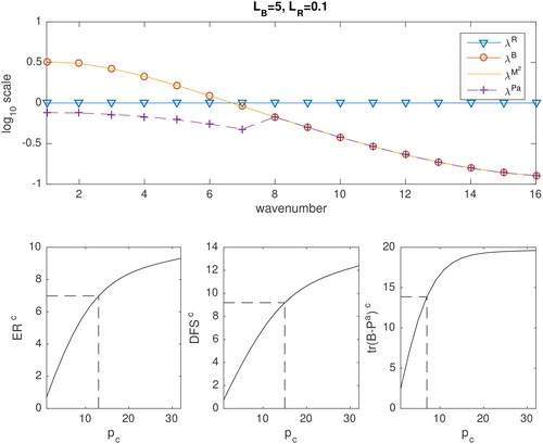
Fig. 2. As in but for The black line of the last panel shows
as a function of the number of compressed observations when the assimilation is performed using large-scale observations first, and the red line when the assimilation is performed using small-scale observations first.
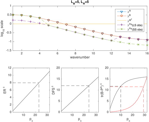
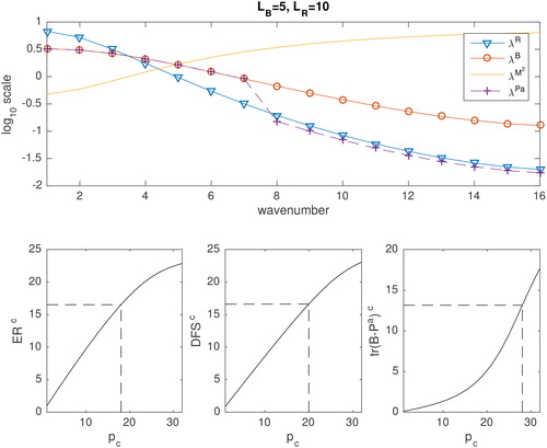
Fig. 3. As in but for
When and we see that the observation uncertainty is 1 at all scales. As the length-scale in
increases the uncertainty of the observations increases at small wave numbers and decreases at large wave numbers. This is consistent with observations with correlated errors providing more information about smaller scales and less about larger scales than observation without correlated errors (Seaman, Citation1977; Rainwater et al., Citation2015; Fowler et al., Citation2018).
Also plotted in the top panels of are the eigenvalues of (yellow line). When
() we see that the eigenvalues of
are greater at small wave numbers and hence large-scale features will be favoured by the data compression. However, when
() we see that the eigenvalues of
are greater at large wave numbers and hence small-scale features will be favoured by the data compression. When
() the eigenvalues of
are constant (i.e. the observations provide the same information about all scales). Therefore, the scales chosen by the data compression are arbitrary.
In the bottom panels of , (left) and
(middle) are shown as a function of the number of compressed observations ordered according to the magnitude of λM. The dashed lines indicate the number of compressed observations needed to achieve 75% of the total value. These numbers are also given in .
Table 1. 75% of the value of ER, DFS, and when all observations are assimilated for different values of
In brackets are the number of compressed observations need to achieve these values.
If we first compare the values of and
when all 32 observations are assimilated we see that both ER and DFS increase as the length-scales in
increases. This is explained in detail in Fowler et al. (Citation2018).
When the information content of the observations initially rises quickly as the number of compressed observations are increased before slowly plateauing as additional observations bring little new information. This means that in these cases less than 75% of the compressed observations are needed to achieve 75% of the information of the total observations. This is obviously not the case when
in which case the information content is proportional to the number of compressed observations.
In the last panel of , is shown as a function of the number of compressed observations, again ordered according to the magnitude of λM. Again the dashed lines indicate the number of compressed observations needed to achieve 75% of the total reduction in error variance (numbers are given in ).
Let us first compare the values of when all 32 observations are assimilated. We see that unlike ER and DFS,
is at a minimum when
This is because both the observations and prior are informative about the same directions of state space, whereas when
the observations and prior have more complimentary information and are more able to reduce the analysis error variances (Fowler et al., Citation2018).
In the case when compressing the observations to maximise information content is also seen to result in the maximum reduction in analysis error variance. In this case, 75% of the reduction in analysis error variance is achievable with just the first 8 compressed observations.
The eigenvalues of the analysis error covariance matrix as a function of wavenumber are plotted in the top panel of (purple crosses) when the compressed observations responsible for 75% of the entropy reduction are assimilated. The reduction in the analysis uncertainty at large scales compared to the background uncertainty is clearly seen.
In the case when we saw previously that it does not matter which of the compressed observations are used to maximise the information content. However, this is clearly not the case if we are interested in reducing the analysis error variance. The black line of the last panel of shows
as a function of the number of compressed observations when the assimilation is performed using large-scale observations first, and the red line when the assimilation is performed using small-scale observations first. It is clear that a few observations of the large-scales (where the background uncertainty is greatest) results in a much smaller analysis error variance than many small-scale observations.
The eigenvalues of the analysis error covariance matrix as a function of wavenumber, for the two different orderings of the compressed observations, are plotted in the top panel of . When 24 compressed observations (chosen as the number needed to retain 75% of the information content) of the large scales are assimilated (purple crosses), the reduction in the analysis uncertainty at large scales compared to the background uncertainty is clearly seen. However, when the first 24 small-scale observations are assimilated (green crosses), the reduction in the analysis uncertainty at small scales compared to the background uncertainty is only visible due to the log scale. This is because the background is already relatively accurate at the small scales.
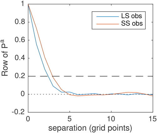
Despite the analysis error variances being smaller when the large-scale observations are assimilated, it is clear that the entropy of the posterior is the same irrespective of the order the compressed observations are assimilated. This is because assimilating the small-scale observations has an important effect on the analysis error correlations, not measured by the trace of the analysis error covariance matrix, and hence the overall entropy is the same in the two cases. The correlation structure for the circulant analysis error covariance matrices are shown in . We see that the correlation length-scales are longer when the small scale observations are assimilated, implying that in this case the relative accuracy of the analysis at small scales to large scales is much greater. In both cases the entropy of is 28.2.
Fig. 4. Analysis error correlation structure for the case illustrated in . The number of compressed observations assimilated are chosen to conserve 75% of ER. Blue: compressed observations favour large scales and red: compressed observations favour small scales.
Lastly, when () it is the small-scale observations which have the greatest information content. However, much more than 75% of these compressed observations are necessary to achieve 75% of the reduction in analysis error variance.
From these simple experiments it can be concluded that as the length-scales in increase and the accuracy of the observations at the smallest resolved scales becomes greater than the background, that there is greater benefit to having a resolution of observations that matches that of the model. Assimilating this quantity of data is however unfeasible for many observation types. To reduce the amount of data for assimilation, data compression may be used to ensure that the most informative combination of observations are retained. It is possible that the optimal combination of observations for retaining the maximum information will not be the same as giving the greatest reduction in analysis error variance, especially when the small scales are favoured over the large scales. This discrepancy between information content and reduction in analysis error variance can be understood by comparing the equation for ER (13) with
ER is sensitive to how the determinant of the error variance matrix changes due to the assimilation of the observations rather than just the trace. ER is therefore much more sensitive to corrections to the relatively accurate small-scales. The relevance of accurately constraining the small-scales is becoming increasingly important for high-resolution forecasting of high-impact weather.
Experiments were performed in which observations are available at a higher resolution than that resolved by the model but in all cases the information content at these unresolved scales was less than at those resolved. As such these unresolved scales would not be chosen during the data compression, despite having some information.
4. Application to the Lorenz 1996 model
In this section, the data compression method described in Section 3 is applied to the Lorenz 1996 model (Lorenz, Citation1995) using the EnKF (described in Section 2) to assimilate the observations.
The Lorenz 1996 model solves the following set of equations
(25)
(25)
where
with n = 40 and F = 8, assuming a cyclic domain. Following Lorenz and Emanuel (Citation1998), a fourth-order Runge-Kutta scheme is used with a time step of 0.05. This toy model represents the evolution of an arbitrary ’atmospheric’ variable in n sectors on a latitude circle. With the forcing term F = 8, the model exhibits chaotic behaviour. The model naturally represents scales associated with the complex sinosoid with the 20 different frequencies that can be represented on the 40 grid points of the model. The largest spatial scale is the average of the variables across the circular domain and the smallest is the complex sinusoid with wavelength of twice the grid spacing.
A simulated true trajectory is generated with initial conditions given by An initial ensemble is generated from
where
In the following experiments B is given by a circulant matrix, with a SOAR correlation function (24) with length-scale
and variance 5. The ensemble size is N = 100. The ensemble is then propagated in time using the Lorenz 1996 model with stochastic forcing at every grid point and time step drawn from a Normal distribution with variances given by 0.01.
40 evenly distributed observations are simulated from the truth run every 20 time steps starting 100 time steps into the simulation (allowing for spin up of the ensemble). where
20 time steps can be thought of as equivalent to 5 days comparing the error doubling time in the Lorenz 1996 model to the real atmosphere (assuming the latter is 2 days) (Khare and Anderson, Citation2006). This frequency of observations is chosen to make the effect of the observations at each assimilation time clearer.
Two observation error covariance matrices are considered given by a circulant matrix with a SOAR correlation function (24) and variance 5. In the first (effectively uncorrelated observation errors). In the second
(giving correlations greater than 0.2 out to about 7 grid points).
Experiments were performed with other parameters for the respective covariance matrices and sampling frequencies, however, there was little sensitivity to these in the qualitative results shown below and the conclusions made are unchanged.
Five methods of data reduction are compared. Those referred to as ‘optimal’ imply that they are dependent upon an objective criterion based on the information content of the observations. In each case only five pieces of observational data are retained for assimilation from the original 40 observations. This dramatic reduction in the data is chosen to highlight the differences between the different methods of data reduction within the numerical experiments. In practice a criteria for retaining a certain proportion of the information of the total observations may be used for choosing the number of compressed observations (as in Section 3.2), or a threshold on the information content of each compressed observation assimilated may be used as in Migliorini (Citation2013). The five methods of data reduction are
Thinning: Observations are thinned to every 8th grid point.
Optimal thinning: Observations are chosen corresponding to the 5 largest diagonal values of
measuring the greatest values of
Spatial averaging: Observations are averaged over 8 grid-points centred on every 8th grid point.
Optimal Fourier Data Compression (DC): Observations are compressed using a Fourier transform with wavelengths chosen corresponding to the 5 largest diagonal values of
Optimal DC: Observations are compressed using the method described in Section 3, again assimilating just the 5 most informative observations.
For each of these methods a compression matrix, is defined and the new observation operators, observations assimilated and their error covariances are computed using (17) to (19). Note that in this case the original observation operator,
was simply the identity matrix.
The observation operators, corresponding to these five compression strategies are shown in . The coloured lines represent the 5 different rows of the
matrix. In the first and third compression strategies, the observation operator is independent of the observation error covariance matrix and time step. In the ‘optimal’ second, fourth and fifth compression strategies, the observation operator is dependent upon the ensemble representation of the prior uncertainties and the full observation error covariance matrix. These are illustrated for the first observation time, so that the prior uncertainty (approximated by the ensemble) is the same in each case. It is seen that when the observation errors are correlated, the optimal data compression retains smaller scale features of the observations, wave-numbers selected by the optimal Fourier decomposition are also shown in . In comparison, the effect of spatial averaging is a severe smoothing out of the small-scale information in the observations.
Fig. 5. Rows of the observation operator matrix for the five strategies for reducing the observation data detailed in Section 4. The optimal strategies are illustrated for the first observation time.
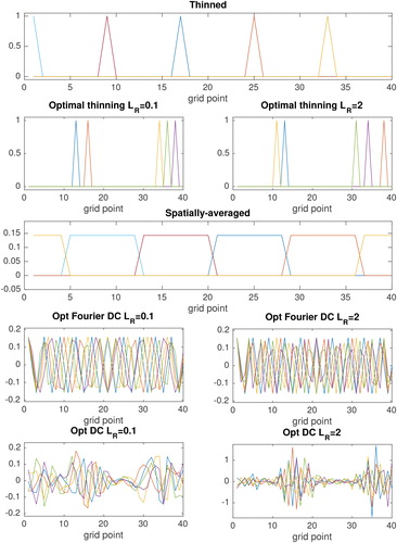
Table 2. The wave-numbers selected by the optimal Fourier data compression method at each observation time for the two different types of observations. The first observation time corresponds to the observation operator plotted in .
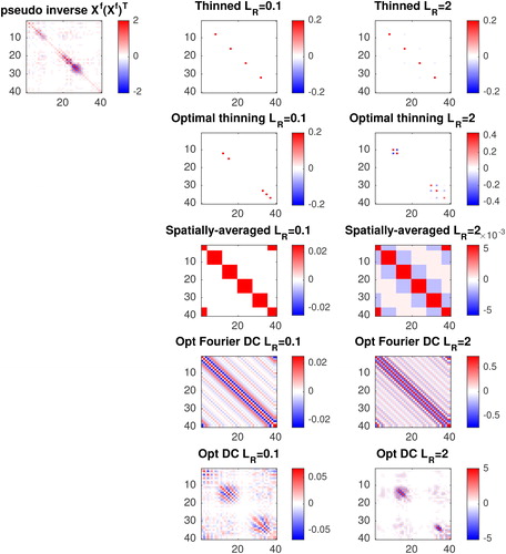
In , the pseudo inverse of and
for the different data reduction strategies are shown for the first observation time. Note that, unlike in Section 3.1,
is no longer circulant. These represent the accuracy of the prior and assimilated observations in state space, respectively. It is seen that the ‘optimal’ thinning and data compression methods choose observations in regions where the prior accuracy is low (i.e. the prior uncertainty is large). When the observation errors are uncorrelated the trace of
is approximately equal to 1 irrespective of data compression strategy. When the observation errors are correlated the trace of
is greatest when observations are compressed using the optimal DC method described in Section 3, and the smallest when they are spatially averaged (47.0 compared to 0.227).
Fig. 6. Top left: pseudo inverse of illustrated for the first observation time. Other panels:
(the accuracy of the compressed observation in state space) for the 5 different thinning strategies when observation errors are uncorrelated (middle panels) and correlated (right panels) illustrated for the first observation time.
The resulting ensemble spread, entropy (estimated from (11) using the ensemble approximation of the error covariance matrix) and ER for the thinning experiments are shown in . In these figures, the values have been averaged over 200 random realisations of the observation and model error. Also plotted in is the condition number of the analysis error covariance matrix, which is related to how sensitive the analysis is to perturbations in the data. The closer this is to 1 the better the conditioned the inverse problem (Golub and Van Loan, Citation1996). The solid lines are when the simulated observations have uncorrelated error and the dashed lines are when the observation errors are correlated.
Fig. 7. (a) Ensemble spread, (b) entropy computed using the ensemble estimate of (11), (c) and (d) log10 of the condition number of the analysis error covariance matrix for the five different thinning strategies detailed in Section 3.1. Solid lines represent results when the observation errors are uncorrelated, dashed lines represent results when the observation errors are correlated. Results are averaged over 200 experiments with different realisations of the observation and model error.
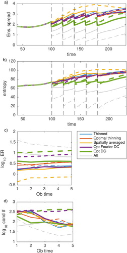
Let us first compare the case when all 40 observations are assimilated (grey lines) every 20 time steps. We see that the observations with correlated errors result in a smaller ensemble spread and entropy than observations with uncorrelated errors. It is interesting to note that after each assimilation time the entropy represented by the ensemble increases most rapidly when the observation errors are correlated. Recall that both the ensemble spread and entropy measure the uncertainty in the ensemble, however, the entropy is sensitive to changes in the correlations in the ensemble perturbations as well as their magnitudes, and hence more representative of the uncertainty at all scales. Therefore, the greater increase in entropy with time for the correlated errors is indicative of the small-scale corrections dissipating during the forecast period between analysis times.
Observations with correlated error are also seen to have significantly more information, as the reduction in entropy is greater at each analysis time. This reduces in time due to the reduction in the ensemble spread (increase in the prior accuracy). Initially, the conditioning is worse when the observation errors are correlated as would be expected (CitationTabeart et al., 2018), however, the opposite is true after the 2nd observation time. This is consistent with the ensemble spread reducing in time and the influence of the observations also reducing (Haben et al., Citation2011).
When the observations are thinned to every 8th grid point (blue lines) the performance of the DA is degraded as would be expected using only 12.5% of the original observations. The difference between the lines is negligible for the different observation error types. This is because the thinning distance of the observations is practically beyond the correlation length-scale.
When the observation errors are uncorrelated, there appears to be little effect on the ER () when the observations are thinned (blue line), spatially averaged (yellow line) or compressed using the optimal Fourier wavelengths (purple line), with numbers ranging between 1.5 and 2.6. There is a slight increase in ER when the optimal thinning (red line) is used (up to approximately 3.8). When the optimum compression is used (green line) there is an increase in ER (increasing to approximately 4.08) and a clear reduction in ensemble spread. When the observation errors are uncorrelated, there is also little difference between the condition number for the five different data reduction strategies.
When the observation errors are correlated the choice of data reduction on the results is much more significant. Compared to thinning the observations (blue dashed-line), spatial averaging (yellow dashed line) is seen to be significantly detrimental to the ER (0.46 compared to 2.8) and ensemble spread. This is because spatial averaging smooths out the highly accurate small scale information of the observations leaving just the less accurate large scale information. Spatial averaging is less detrimental when observation errors are uncorrelated as in this case the observations provide the same information at all scales (see ), and averaging enables a reduction in the noise. Again there is a slight increase in ER when the optimal thinning (red dashed line) is used (3.7 compared to 2.8).
Using the Fourier compression or the optimal data compression, when the observation errors are correlated is seen to lead to a large increase in ER (greater, in many cases, than using the full 40 observations when the errors are uncorrelated). In , we saw that both these methods of data compression are selecting the fine scale information in the observations for assimilation.
The reason that the ensemble spread is smaller when the observations have uncorrelated error compared to correlated error with the optimal DC may be related to the results shown in Section 3.2. It was seen here that using observations to correct the small scales was less able to reduce the analysis error variance, which is approximated by the ensemble spread, despite the information content of the observations being greater. This hypothesis is supported by the entropy time series where it is seen that at each observation time the entropy of the posterior is actually smaller when assimilating the optimally compressed observations with correlated error rather than uncorrelated error. Increasing the number of compressed observations (and hence the number of scales retained by the data compression) sees the ensemble spread quickly reduce. For example, when just 8 of the compressed observations are retained, the ensemble spread when the observations have correlated errors is smaller than the ensemble spread when the observation errors are uncorrelated by the fifth observation time (results not shown).
In the case when the observation errors are correlated, the condition number is much larger when using these more optimal methods of data compression. This could potentially have an undesirable impact on the sensitivity of the analysis to perturbations in the data.
5. Summary and conclusions
Recent advances in the estimation and inclusion of OECs in DA means that we are getting closer to be able to assimilate denser observations with an accurate description of their uncertainty. As observations with correlated error are known to have greater information at small scales than observations with uncorrelated error this may be crucial for high resolution forecasting in which accurate forecasts of small-scale high impact weather are sought.
This may seem contradictory to previous studies of Liu and Rabier (Citation2002) and Bergman and Bonner (Citation1976) that concluded that increasing the density of observations with correlated error is not as beneficial as if the observations had uncorrelated error, due to the reduction in analysis RMSE not being as great. This is, in part, due to the effect of increasing the correlation length-scales of the observation errors bringing the likelihood PDF more in line with the prior PDF (Fowler et al., Citation2018). Once the OEC length-scales are increased beyond those of the prior, the reduction in analysis RMSE with increasing observation density is seen to increase once again.
The potential large increase in the number of observations available for assimilation carries a large computational and storage burden with it. It is therefore important to justify any increase in the amount of data assimilated and give careful thought to the design of the observing network. One way to potentially reduce the computational burden is to reduce the data using a compression technique based on retaining the maximum information content of the observations.
In an idealised circulant framework it was shown how the scales that are retained by the data compression depends upon the structure of the prior and OECs. When the length-scales in R are smaller than those in B, observations of large-scale features are retained for assimilation. When the length-scales in R are greater than those in B, observations of small-scale features are retained for assimilation. However, the greater the length-scales in R, the greater the total information content of those observations.
It was shown that, despite possibly having greater information content, many more small-scale observations are needed than large-scale observations to achieve the same level of reduction in the analysis error variances. This highlights a potential discrepancy between information content (a relative quantity) and reduction in the analysis error variances (an absolute quantity). The importance of constraining the analysis at small-scales depends upon the aim of performing the assimilation. For the increasingly important applications of high-impact forecasting that aim to produce limited area forecasts out to short lead times, corrections to the small-scales are arguably more important than correcting the large-scales. In these cases the large-scales are largely constrained by the boundary conditions provided by the global model. It is only when forecasting at longer lead times that the small scale corrections in the analysis dissipate and become invaluable. In addition to this, large scale information may be available from other observations. Therefore, to understand the full potential of observations with correlated errors it is important not to concentrate only on the effect on the reduction in the analysis error variances or analysis RMSE.
In Section 3.1, the compression of the observations was then applied to the EnKF using the Lorenz 1996 model, for observations with correlated and uncorrelated errors. The data compression method was compared to other methods to reduce the amount of data. These included regular thinning, optimal thinning (in which the observations with the greatest analysis sensitivities where selected), spatial averaging, and compression using a Fourier transform based on the wavelengths with the greatest analysis sensitivity.
It was found that when the observation errors are uncorrelated, the information content of the reduced data set is largely insensitive to the strategy used. However, when the observation errors are correlated, it is found that the information content of the reduced data set is highly sensitive to the strategy used. In particular using a data compression method based on maximising the information content of the compressed observations can increase the entropy reduction of the reduced observations by up to 420% compared to regular thinning. Whereas observations reduced using spatial averaging have only 16% of the entropy reduction of observations reduced using regular thinning.
This implies that when the observations have correlated error it is more beneficial to have high-density observations. However, in order to reduce the amount of data, the use of spatial averaging can be more detrimental than regular thinning and instead data compression based on retaining the small-scale information should be used. The need for this to be performed on-line depends on how quickly the length scales of the correlations represented by the ensemble are evolving.
In the Lorenz 1996 example, although the optimal methods were adaptive with the changing flow of the ensemble, the compression was actually relatively static (see for an example of the how the most important wave numbers change for the 5 observation times). Future work will look further at the effect of the flow dependent estimate on the data compression using a more physically realistic model in which prior error correlations are more dynamic. For example, using the multivariate modified shallow water model of Kent et al. (Citation2017) which represents simplified dynamics of cumulus convection and associated precipitation, and the corresponding disruption to large-scale balances. Methods for reducing the computational cost of on-line data compression will also be investigated, as well as the possibility of retaining some base line scales.
In practice the use of data compression can be expected to be sensitive to the accuracy of the specified error characteristics. This will be the focus of future work. The results could also be sensitive to the way the ensemble Kalman filter is implemented (e.g. ensemble size, localisation, inflation, etc.). Experiments were also performed with a small ensemble size of N = 10 with little effect on the results, largely because, even in this case, the number of compressed observations () was less than N. The sensitivity to the ensemble parameters can be expected to increase as
increases.
Acknowledgements
I would like to thank J. Eyre (UK Met Office), R. N. Bannister and J. A. Waller (Uni. Reading) for providing valuable feedback and discussion.
Additional information
Funding
Related Research Data
References
- Berger, H. and Forsythe, M. 2004. Satellite wind superobbing. Met Office Forecasting Research Technical Report No. 451. http://research.metoffice.gov.uk/research/nwp/publications/papers/technical_reports
- Bergman, K. H. and Bonner, W. D. 1976. Analysis error as a function of observation density for satellite temperature soundings with spatially correlated errors. Mon. Wea. Rev. 104, 1308–1316. doi:10.1175/1520-0493(1976)104<1308:AEAAFO>2.0.CO;2
- Bormann, N. and Bauer, P. 2010. Estimates of spatial and interchannel observation-error characteristics for current sounder radiances for numerical weather prediction. I: methods and application to ATOVS data. Q. J. R. Meteorol. Soc. 136, 1036–1050. doi:10.1002/qj.616
- Bormann, N., Saarinen, S., Kelly, G. and Thépaut, J.-N. 2003. The spatial structure of observation errors in atmospheric motion vectors from geostationary satellite data. Mon. Wea. Rev. 131, 706–718. doi:10.1175/1520-0493(2003)131<0706:TSSOOE>2.0.CO;2
- Bormann, N., Bonavita, M., Dragani, R., Eresmaa, R., Matricardi, M. and co-authors. 2016. Enhancing the impact of IASI observations through an updated observation-error covariance matrix. Q. J. R. Meteorol. Soc. 142, 1767–1780. doi:10.1002/qj.2774
- Campbell, W. F., Satterfield, E. A., Ruston, B. and Baker, N. L. 2017. Accounting for correlated observation error in a dual formulation 4D-variational data assimilation system. Mon. Wea. Rev. 145, 1019. doi:10.1175/MWR-D-16-0240.1
- Cardinali, C., Pezzulli, S. and Andersson, E. 2004. Influence-matrix diagnostics of a data assimilation system. Q. J. R Meteorol. Soc. 130, 2767–2786. doi:10.1256/qj.03.205
- Collard, A. D., McNally, A. P., Hilton, F. I., Healy, S. B. and Atkinson, N. C. 2010. The use of principal component analysis for the assimilation of high-resolution infrared sounder observations for numerical weather prediction. Q. J. R. Meteorol. Soc. 136, 2038–2050. URL https://rmets.onlinelibrary.wiley.com/doi/abs/10.1002/qj.701. doi:10.1002/qj.701
- Cordoba, M., Dance, S. L., Kelly, G. A., Nichols, N. K. and Waller, J. A. 2017. Diagnosing atmospheric motion vector observation errors for an operational high resolution data assimilation system. Q. J. R. Meteorol. Soc. 143, 333–341. doi:10.1002/qj.2925
- Dando, M. L., Thorpe, A. J. and Eyre, J. R. 2007. The optimal density of atmospheric sounder observations in the Met Office NWP system. Q. J. R. Meteorol. Soc. 133, 1933–1943. doi:10.1002/qj.175
- Evensen, G. 1994. Sequential data assimilation with a nonlinear quasi-geostrophic model using Monte Carlo methods to forecast error statistics. J. Geophys. Res. 99, 10143–10162. doi:10.1029/94JC00572
- Fowler, A., Dance, S. and Waller, J. 2018. On the interaction of observation and a-priori error correlations. Q. J. R. Meteorol. Soc. 144, 48–62. doi:10.1002/qj.3183
- Fowler, A. M. 2017. A sampling method for quantifying the information content of IASI channels. Mon.Wea. Rev. 145, 709–725. doi:10.1175/MWR-D-16-0069.1
- Goldberg, M. D., Qu, Y., McMillin, L. M., Wolf, W., Zhou, L. and Divakarla, M. 2003. AIRS near-real-time products and algorithms in support of operational numerical weather prediction. IEEE Trans. Geosci. Remote Sensing 41, 379–389. doi:10.1109/TGRS.2002.808307
- Golub, G. H. and Van Loan, C. F. 1996. Matrix Computations. 3rd ed. The John Hopkins University Press, Baltimore, MD.
- Gray, R. 2006. Toeplitz and Circulant Matrices: A Review. Foundations and Trends in Communications and Information Theory: Vol 2: No. 3, pp 155–239. doi:10.1561/0100000006
- Haben, S. A., Lawless, A. S. and Nichols, N. K. 2011. Conditioning of incremental variational data assimilation, with application to the Met Office system. Tellus A 64, 782–792.
- Hamill, T. M., Whitaker, J. S. and Snyder, C. 2001. Distance-dependent filtering of background error covariance estimates in an ensemble Kalman filter. Mon. Wea. Rev. 129, 2776–2790. doi:10.1175/1520-0493(2001)129<2776:DDFOBE>2.0.CO;2
- Hilton, F., Collard, A., Guidard, V., Randriamampianina, R. and Schwaerz, M. 2009. Assimilation of IASI radiances at European NWP centres. In: Proceedings of Workshop on the assimilation of IASI data in NWP, ECMWF, Reading, UK, 6-8 May 2009.
- Houtekamer, P. L. and Zhang, F. 2016. Review of the ensemble Kalman filter for atmospheric data assimilation. Mon. Wea. Rev. 144, 4489–4532. doi:10.1175/MWR-D-15-0440.1
- Huang, H.-L. and Purser, R. J. 1996. Objective measures of the information density of satellite data. Meteorl. Atmos. Phys. 60, 105–117. doi:10.1007/BF01029788
- Hunt, B. R., Kostelich, E. J. and Szunyogh, I. 2007. Efficient data assimilation for spatiotemporal chaos: a local ensemble transform Kalman filter. Physica D 230, 112–126. doi:10.1016/j.physd.2006.11.008
- Janjic, T., Bormann, N., Bocquet, M., Carton, J. A., Cohn, S. E. and co-authors. 2017. On the representation error in data assimilation. Q. J. R. Meteorol. Soc. 144, 1257–1278. doi:10.1002/qj.3130
- Kalnay, E. 2003. Atmospheric Modeling, Data Assimilation and Predictability. Cambridge University Press, New York,.
- Kent, T., Bokhove, O. and Tobias, S. 2017. Dynamics of an idealized fluid model for investigating convective-scale data assimilation. Tellus A 69, 1369332. URL doi:10.1080/16000870.2017.1369332
- Khare, S. P. and Anderson, J. L. 2006. An examination of ensemble filter based adaptive observation methodologies. Tellus 58A, 179–195.
- Li, Z., Ballard, S. P. and Simonin, D. 2018. Comparison of 3D-Var and 4D-Var data assimilation in an NWP-based system for precipitation nowcasting at the Met Office. Q. J. R. Meteorol. Soc. 144, 404–413. URL https://rmets.onlinelibrary.wiley.com/doi/abs/10.1002/qj.3211. doi:10.1002/qj.3211
- Liu, Z.-Q. and Rabier, F. 2002. The interaction between model resolution, observation resolution and observational density in data assimilation: a one-dimensional study. Q. J. R. Meteorol. Soc. 128, 1367–1386. doi:10.1256/003590002320373337
- Liu, Z.-Q. and Rabier, F. 2003. The potential of high-density observations for numerical weather prediction: a study with simulated observations. Q. J. R. Meteorol. Soc. 129, 3013–3035. doi:10.1256/qj.02.170
- Lorenz, E. N. 1995. Predictability – a problem partly solved. In: Seminar Proceedings I, Reading, UK, ECMWF, pp. 1–18.
- Lorenz, E. N. and Emanuel, K. A. 1998. Optimal sites for supplementary weather observations: simulation with a small model. J. Atmos. Sci. 55, 399–414. doi:10.1175/1520-0469(1998)055<0399:OSFSWO>2.0.CO;2
- Majumdar, S. J. 2016. A review of targeted observations. Bull. Am. Meteor. Soc. 97, 2287–2303. URL doi:10.1175/BAMS-D-14-00259.1
- Migliorini, S. 2013. Information-based data selection for ensemble data assimilation. Q. J. R. Meteorol. Soc. 139, 2033–2054. doi:10.1002/qj.2104
- Migliorini, S. 2015. Optimal ensemble-based selection of channels from advanced sounders in the presence of cloud. Mon. Wea. Rev. 143, 3754–3773. URL doi:10.1175/MWR-D-14-00249.1
- Miyoshi, T., Lien, G.-Y., Satoh, S., Ushio, T., Bessho, K. and co-authors. 2016. Big data assimilation” toward post-petascale severe weather prediction: An overview and progress. Proc. IEEE 20, 2155–2179.
- Oke, P. R., Sakov, P. and Corney, S. P. 2007. Impacts of localisation in the EnKF and EnOI: experiments with a small model. Ocean Dyn. 57, 32–45. doi:10.1007/s10236-006-0088-8
- Rabier, F., Jarvinen, H., Klinker, E., Mahfouf, J.-F. and Simmons, A. 2000. The ECMWF operational implementation of four-dimensional variational data assimilation. I: experimental results and simplified physics. Q J. R. Meteorol. Soc. 126, 1143–1170. doi:10.1002/qj.49712656415
- Rabier, F., Fourrié, N., Chafa I, D. and Prunet, P. 2002. Channel selection methods for infrared atmospheric sounding interferometer radiances. Q J. R Meteorol. Soc. 128, 1011–1027. doi:10.1256/0035900021643638
- Rainwater, S., Bishop, C. H. and Campbell, W. F. 2015. The benefits of correlated observation errors for small scales. Q. J. R. Meteorol. Soc. 141, 3439–3445. doi:10.1002/qj.2582
- Rawlins, F., Ballard, S. P., Bovis, K. J., Clayton, A. M., Li, D. and co-authors. 2007. The Met Office global four-dimensional variational data assimilation scheme. Q. J. R. Meteorol. Soc. 133, 347–362. doi:10.1002/qj.32
- Rodgers, C. D. 2000. Inverse Methods for Atmospheric Sounding. World Scientific Publishing, Singapore.
- Seaman, R. S. 1977. Absolute and differential accuracy of analyses achievable with specified observational network characteristics. Mon. Wea. Rev. 105, 1211–1222. doi:10.1175/1520-0493(1977)105<1211:AADAOA>2.0.CO;2
- Stewart, L. M., Dance, S. L., Nichols, N. K., Eyre, J. R. and Cameron, J. 2014. Estimating interchannel observation-error correlations for IASI radiance data in the Met Office system. Q. J. R. Meteorol. Soc. 140, 1236–1244. doi:10.1002/qj.2211
- Tabeart, J. M., Dance, S. L., Haben, S. A., Lawless, A. S., Nichols, N. K. and co-authors. 2018. The conditioning of least squares problems in variational data assimilation. Numer. Linear Algebra Appl. 0, e2165. URL https://onlinelibrary.wiley.com/doi/abs/10.1002/nla.2165.
- van Leeuwen, P. J. 2015. Representation errors and retrievals in linear and nonlinear data assimilation. Q. J. R. Meteorol. Soc 141, 612–1623.
- Waller, J. A., Dance, S. L., Lawless, A. S. and Nichols, N. K. 2014. Estimating correlated observation error statistics using an ensemble transform Kalman filter. Tellus A 66, 23294. doi:10.3402/tellusa.v66.23294
- Waller, J. A., Ballard, S. P., Dance, S. L., Kelly, G., Nichols, N. K. and co-authors. 2016a. Diagnosing horizontal and inter-channel observation error correlations for SEVIRI observations using observation-minus-background and observation-minus-analysis statistics. Remote Sens. 8, 581. doi:10.3390/rs8070581
- Waller, J. A., Simonin, D., Dance, S. L., Nichols, N. K. and Ballard, S. P. 2016b. Diagnosing observation error correlations for Doppler radar radial winds in the Met Office UKV model using observation-minus-background and observation-minus-analysis statistics. Mon. Wea. Rev. 144, 3533. doi:10.1175/MWR-D-15-0340.1
- Weston, P. P., Bell, W. and Eyre, J. R. 2014. Accounting for correlated error in the assimilation of high-resolution sounder data. Q. J. R. Meteorol. Soc. 140, 2420–2429. doi:10.1002/qj.2306
- Xu, Q. 2007. Measuring information content from observations for data assimilation: relative entropy versus Shannon entropy difference. Tellus 59A, 198–209.
- Xu, Q., Wei, L. and Healy, S. 2009. Measuring information content from observations for data assimilation: connection between different measures and application to radar scan design. Tellus 61A, 144–153.