Using statistical downscaling to assess skill of decadal predictions

Abstract

We test a hypothesis that the signal-to-noise ratio of decadal forecasts improves with larger scales and can be utilised through model output statistics (MOS) involving empirical-statistical downscaling and dependencies to large-scale conditions. Here, we used MOS applied to an ensemble of decadal forecasts to predict local wet-day frequency, the wet-day mean precipitation, and the mean temperature for one to nine year long intervals of forecasts with a one year lead time. Our study involved a set of decadal forecasts over the 1961–2011 period, based on a global coupled ocean-atmosphere model that was downscaled and analysed for the North Atlantic region. The MOS for the decadal forecasts failed to identify aspects that were associated with higher skill for temperature and precipitation over Europe on time scales shorter than five years. A likely explanation for not enhancing skillful parts of the forecasts was that the raw model output had low skill for the general large-scale atmospheric circulation. This was particularly true for the wet-day frequency over Europe, which had a strong connection to the mean sea-level pressure (SLP) anomalies over the North Atlantic. There was a weak connection between large-scale maritime surface temperature anomalies and local precipitation and temperature variability over the European continent. The decadal forecasts for time scale of nine years and longer, on the other hand, exhibited moderate skill. The dependency between temporal and spatial scales was found to differ for the temperature and the mean SLP anomalies, but we found little indication that the decadal predictions for anomalies with large-scale regional extent were associated higher skill than for more local patterns in these forecasts.

Keywords:

• model output statistics
• downscaling
• decadal predictions
• common EOFs

1. Introduction

Decadal predictions are at the forefront of climate research whereby global climate models (GCMs) involving coupled atmospheric and oceanic components are initialised with the best available information about the current state of the oceans and subsequently used to simulate the next decade or so (Meehl et al., 2014). GCMs have more traditionally been used for climate change projections to provide a picture of a climate several decades into the future (Chang et al., 2012), and although they also can produce simulations for the near future, they typically do not start with initial conditions that match the current state of the ocean and atmosphere. Because climate projections usually do not involve initial conditions that provide the best snapshot of current conditions, a large fraction of the uncertainty in the Atlantic in the first few decades is likely due to internal variability, as suggested by uncertainty partitioning (Hawkins and Sutton, 2009). Recent results from model experiments indicate some decadal predictive skill in the North Atlantic (Doblas-Reyes et al., 2013; Kirtman et al., 2013; Garca-Serrano et al., 2015), western Pacific (Mochizuki et al., 2010; Chikamoto et al., 2015) and the Indian Ocean (Guemas et al., 2013), however, the skill is lower in other regions of the world’s oceans. One cause of long-term predictability may be a result of the slow advection of heat in the Atlantic Ocean (Sutton and Allen, 1997; Robson et al., 2014); however, there may potentially also be other slow physical processes that play a role in the North Atlantic, and it is this internal variability that decadal forecasts try to predict.

GCMs are designed to simulate large-scale features and have a minimum skillful scale that may be of the order of a few grid-boxes (Takayabu et al., 2016). Downscaling is required to represent smaller-scale features and involves a variety of methods that utilise dependencies between large-scale and small-scale processes and conditions. It includes both nested high-resolution limited area models (also referred to as ‘dynamical downscaling’) as well as statistical methods as in empirical-statistical downscaling (ESD) (Takayabu et al., 2016). ESD uses statistical methods such as regression on empirical data (historical observations) to calibrate a simple model that describes the dependency between the large-scale predictor and the small-scale predictand. It can be tailored specifically to particular needs, and so-called model output statistics (MOS) represents one type of ESD where the downscaling models are calibrated with a combination of GCM output and local observations (Wilks, 1995). The benefit with MOS and calibrating the model output against the observations is that it can correct for systematic biases, e.g. if the anomalies are too weak or strong or if the action is systematically displaced in space. Moreover, MOS is a subcategory of ESD, but where the model results are used in the calibration of the downscaling models rather than a third data set (e.g. reanalyses). Hence, the difference between MOS and ‘traditional’ ESD is that the former uses model output as predictors in the calibration of the downscaling models against historical observations, whereas the latter uses historical observations as predictors.

1.1. Current status

Most work on decadal forecasts has so far been based on direct model output and ensembles of GCM output from a single or multiple models. For instance, Meehl et al. (2014) provided a comprehensive review of decadal forecasting, but did not address potential benefits associated with ESD or MOS when applied to such forecasts. Likewise, traditional validation of seasonal-to-decadal forecasts tend to involve direct comparison with reanalyses or observations (Smith et al., 2013; Guemas et al., 2015) or estimation of reliability of the Brier score (Wilks, 1995), however, statistical post-processing, such as ESD or MOS, may potentially enhance the forecast skills as it potentially can by-pass systematic bias and deterioration from local small-scale noise. Some large-scale features may be more predictable than others and may enhance predictive skills if used as predictors in ESD. Furthermore, there is a minimum skillful scale connected to the design of climate models and their ability to represent real-world phenomena and processes. Hibino and Takayabu (2016) studied the effect of aggregating simulated daily precipitation over different temporal and spatial scales on the signal-to-noise ratio (SNR) for the detection of change, and reported increased SNR with longer scales. Improved ability for detecting signal with greater scales can be exploited for decadal forecasts, as it is expected that ESD and MOS emphasise the large-scales, which may be more predictable than small-scale variability, and hence may potentially enhance the prediction skills by filtering out small-scale noise.

There have been few scientific studies where downscaling has been applied to seasonal or decadal forecasts (Caron et al., 2014; Benestad and Mezghani, 2015), but the limited literature may be due to few available seasonal-to-decadal forecasts. It is possible to use ESD and MOS as a diagnostic tool to assess connections between large and small scales, and here ESD was used for checking the link between the scales in the historical data, whereas MOS was used to evaluate the skill of the decadal forecasts. MOS may offer a value-added contribution as model drift from initial state is a difficult obstacle when it comes to decadal forecasting (Meehl et al., 2014). Bias adjustment has often been used to produce skillful forecasts (Kharin et al., 2012), however, it is possible to by-pass a bias adjustment altogether through MOS. In addition to using MOS as an analytical tool for evaluating decadal forecasts, we also used MOS to provide an answer to the question of whether the use of downscaling improves the decadal forecast quality over the raw model output.

The objective of this study was to downscale the wet-day mean precipitation (μ) and the wet-day frequency (f_w), as in Benestad and Mezghani (2015). Here, we assumed a wet day was when more than 1 mm/day precipitation was recorded in a rain gauge measurement. These quantities can be used in probabilistic forecasts since the probability of heavy precipitation may be approximated by an exponential distribution where $\mathit{Pr}(X>x)=f_w{e}^{-x/\mu }$ (Benestad, 2007; Benestad and Mezghani, 2015) (here x is the daily precipitation amount). Furthermore, the total precipitation amount is the product of the two and the total number of days (n): $p_{\mathit{tot}}=n{f}_w\mu$. The greatest potential for downscaling such probabilities appears to be the connection between the mean sea-level pressure (SLP) and f_w, as the connection between the amounts μ and the large-scale conditions may be more complicated (Benestad and Mezghani, 2015). The wet-day frequency responds more to shorter time scales (about 5 years) than the wet-day mean precipitation (about 15 years and longer). A comprehensive analysis of skill needs to account for different time scales and was in this case carried out for annual time scales, three-year aggregates, pentads (five-year means) and nine-year periods.

2. Method

To test whether there is a link between large-scale surface air temperature (TAS) or mean SLP anomalies and local precipitation statistics, ESD was first applied with predictors from the NCEP/NCAR reanalysis 1 over the period 1950–2017 (Kalnay et al., 1996). The predictands (wet-day mean μ and frequency f_w) were aggregated over the forecast interval as in Benestad and Mezghani (2015), but were based on the EOBS (version 19.0) gridded precipitation and temperature data for the period 1950–2017 (Linden and Mitchell, 2009). Here, the term ‘forecast interval’ refers to the number of years ahead that each forecast was extended from the initial lead time, e.g. for an interval of one year we used the annual mean temperature and for a three-year interval we used the three-year average. A more precise mathematical formulation of the forecasted quantity is $\overline{x(t)}, t\in [t_1, t_2]$ where t₁ is the lead time (one year for all the cases presented here) and t₂ is the last date of the forecasted quantity. The forecasts were aggregated to estimate a mean value for the interval in order to represent the associated time scale. Likewise, corresponding aggregated quantities were estimated from the EOBS data. The validation involved a leave-one-out (LOO) cross-validation (Wilks, 1995). Since past studies suggest that the circulation pattern seems to affect the frequency of rainy days, we used SLP as predictor for f_w (Benestad and Mezghani, 2015; Benestad et al., 2016). For μ, we tried predictors that could capture the sources of moisture (evaporation), which included the TAS and the saturation water vapour pressure e_s (see the Appendix for more details).

The ensemble mean forecasts were based on the GFDL-CM2.1 model (Delworth et al., 2006) and assessed against the NCEP/NCAR reanalysis to indicate what skill could be expected from the MOS. The assessment of the decadal forecasts involved (i) calculating the correlation between the ensemble mean forecast and the reanalysis, and (ii) a diagnostic of the ensemble spread. For the former, the correlation was estimated over the years of forecasts for each matching pair of grid-boxes in the reanalysis and ensemble means forecast without accounting for the initial drift associated with the prescription of initial conditions. The correlation score should not be sensitive to differences in the mean as long as the drift was similar for the entire set of forecasts for one given forecast interval.

The ensemble spread, on the other hand was quantified through the application of common empirical orthogonal functions (EOFs) (Barnett, 1999; Benestad, 2001). We used common EOFs to quantify the ensemble spread because they provide an elegant and suitable method for comparing different multivariate datasets (Benestad et al., 2017). Common EOFs have not been used much previously within the climate research community for comparing multivariate datasets. Here, they were used to identify the spatial pattern that explains most of the variance within the ensemble and the time evolution associated with this for each of the ensemble members. Here, the term EOF refers to the spatial pattern whereas the principal component (PC) is the time series describing its evolution over time. Combined, the EOFs and PCs bear some similarity with the Fast Fourier Transform because it is possible to reconstruct the original data from the set of EOFs, singular values and PCs.

The common EOFs provided a basis for the MOS where the PCs associated with forecast ensemble were used as input (predictors) in a stepwise multiple regression analysis against the predictand representing local precipitation and temperature. The predictands were also PCs, but were associated with the EOFs of the gridded EOBS data. For the decadal forecasts, there were 10 different predictions (i.e. 10 ensemble members) for the same date/year, whereas for the observations, there was only one data point for each date. To make use of all the information embedded in the ensemble in the evaluation of the forecasts, the same set of observations had to be matched with each ensemble member. We also made use of a multiple regression analysis to assess how well the forecasts matched the observations. Each member of the forecast ensemble (predictors) was included in the regression analysis by creating a joint data matrix made up with concatenated forecasts sorted according to the date (see the Appendix). Each member was matched with corresponding observations by repeating the same observations (predictands) for each ensemble member. The motivation for using a regression with multiple ensemble members was that a large spread was expected to affect the calibration of the stepwise multiple regression used in the MOS in a similar fashion as a high noise fraction, and hence lower the expected variance captured by the regression model.

We expected that the decadal predictability resided in the oceans rather than over land, however, the variability in temperature was greater over land with more pronounced short-term variability and contained more noise. Hence, the experiments were repeated with a land-sea mask to leave out the contribution from land surfaces to assess the ensemble spread in the maritime temperatures.

The application of MOS was designed to emphasise the large scales and their effect on the local conditions, and one potential benefit in using MOS was to increase the SNR if the large scales were more skillfully predicted than the small scales. In this case, the decadal forecasts (TAS, SLP or e_s derived from TAS) were used as predictors in both the calibration process as well as for prediction, and the MOS was based on a stepwise multiple regression analysis, which could account for systematic biases in the forecast fields (e.g. different means/drift, variance or variations offset in space).

The question of how scales are related in time and space has not yet been settled, and a range of different forecast intervals was tested to cover phenomena that are potentially associated with various time scales. For instance, do changes need longer time if they involve larger areas and spatial scales? A related issue was the question of how robust were the forecast skill estimates, which was explored through a comparison of different time scales (prediction period over which the mean was estimated). The assessment therefore involved many trials with different intervals over which the forecasts were aggregated. The question concerning the dependency between temporal and spatial scales was explored in terms of a spectral analysis applied to regional averages from the reanalysis over a range of domains with different area. The smallest domain was taken to be grid box centred in the Atlantic (15${}^{°}$ W/30${}^{°}$ N) and the larger domains were taken to be centred around this grid box (each region i contains ${(2i+1)}^2$ grid boxes where $i\in [0, 1, 2,\dots ]$). Time series were estimated for each of these by taking the area average, which were then used to estimate the power spectra for the different domain sizes.

In summary, the steps taken in this study were:

• Compare variance in TAS and SLP associated with various spatial and temporal scales to assess the presence of large-scale slow processes that may be predictable.

• Aggregate annual f_w and μ for gridded precipitation and the annual mean for the gridded temperature (EOBS).

• Apply ESD to reanalyses and gridded precipitation to assess dependencies to large-scale SLP, TAS or e_s.

• Generate maps of correlation between reanalysis and the forecasts filtered through a limited number of EOFs to assess skill associated with spatial scales.

• Generate common EOFs from data matrices that combine (reanalyses and) all members of the ensemble for analysis and use in MOS.

• Apply MOS to the common EOFs to downscale the aggregated statistics from EOBS and assess predictive skill and account for biases/drift.

More information about the method is provided in the Appendix.

3. Results

3.1. Scale dependency

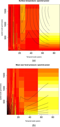
The first part of the study involved an evaluation of how the variance varies with temporal and spatial scales. Results from the scale analysis would provide a context for the subsequent evaluation of the decadal forecasts and the MOS results. We used spectral analyses for comparing the temporal and spatial scales, and Fig. 1a shows results for the power spectra for the surface temperature applied to successively larger domains, and the results indicated pronounced power for a combination of long time scales averaged over a large area. The long-term variability over large regions was consistent with a general warming trend; however, the results also suggested that large-scale fluctuations were associated with ∼20 year time scales. For SLP, on the other hand (Fig. 1b), most of the spectral power was found on the spatial small scales. This reflects shifts in the mass of the air column, which is more pronounced over smaller than over larger volumes. These results provided some support for the initial assumption and one motivation for using MOS in conjunction with decadal forecasts: large-scale temperature anomalies tend to be associated with longer time scales (higher values in the upper right section). For SLP, on the other hand, the most pronounced variations tend to be associated with synoptic cyclones and smaller spatial scales (higher values in the lower section) (Neu, 2012).

Fig. 1. Heat maps showing power spectra along the x-axis for different spatial scales along the y-axis for TAS (a) and SLP (b). Yellow colour signifies high and red low power. The temporal scales are given as months and the area as number of grid boxes. The contours give a smoother representation of the colour scaling. Data: NCEP/NCAR reanalysis 1.

3.2. Link between large and small scale conditions

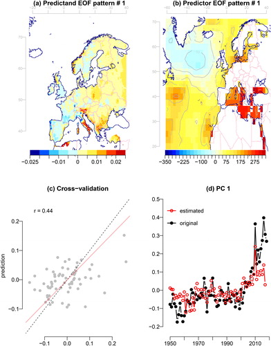
Establishing how spatial scales are connection to variability is a prerequisite for downscaling approaches such as MOS, which makes use of large-scale conditions (predictors) and how the local scales (predictands) depend on these. To make this assessment, we used ESD as a diagnostic tool, as the application of MOS to decadal forecasts was based on the assumption that the local precipitation statistics depends on the large-scale conditions. This assumption was first tested by applying conventional ESD to the NCEP/NCAR reanalysis 1 and the gridded precipitation parameters μ and f_w from the EOBS data. Hence, the first step to assess the effect of applying MOS to decadal forecasts did not involve MOS but a downscaling exercise between the best representation of actual large-scale conditions from a reanalysis and aggregated historical rainfall statistics. The results suggested that there was indeed a connection between the large scales and local precipitation statistics, and Fig. 2 shows the results of a LOO cross-validation for the wet-day frequency. The figure only shows the results for the leading predictand EOF, however, we carried out a multiple regression for each of the four leading predictands PC respectively, using a set of seven predictor PCs as input. There was a particularly close association between the large-scale SLP and the wet-day frequency f_w (LOO correlation of 0.81), but a similar cross-validation analysis suggested more modest skills for the wet-day mean μ when using the saturation vapour pressure e_s over the ocean as the predictor (LOO correlation of 0.44; Fig. 3). Here, only the results for the leading predictand EOF is shown as the higher order patterns were associated with lower proportion of the total covariance (see the Appendix). In addition to that, the cross-validation gave low skill scores for μ, the ESD-based reproduction of the leading EOF pattern for μ did not capture the observed trend associated with this pattern. The maritime TAS and the vapour saturation pressure e_s, which is a function of TAS, were both related to the sea surface temperature (SST), and the predictor pattern for e_s associated with higher μ over Europe exhibited stronger weights in the Mediterranean and the western part of the Atlantic. In summary, the results from both the spectral analysis of scales and the ESD on historical observations indicated that MOS potentially might be a feasible strategy for improving decadal forecasts.

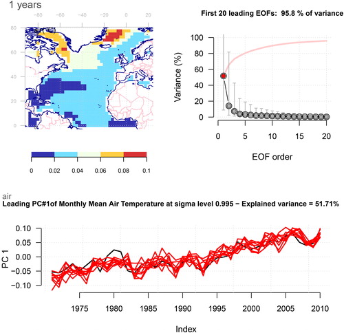
Fig. 2. Results from downscaling wet-day frequency indicated a close association between large-scale annual mean SLP anomalies and variations in the leading EOF of the annual f_w. The upper left panel shows the pattern of the leading EOF estimated for the annual f_w, upper right shows the SLP anomalies which are associated with variations in the leading PC (combination of spatial weights from a stepwise multiple regression) derived from NCAR/NCEP reanalysis 1 SLP, lower left shows a scatter plot between the original PC and predictions in terms of LOO cross-validation, and the lower right shows the original time series (black) and the calibrated results (red).

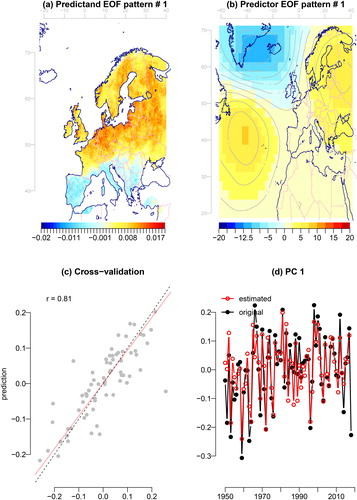
Fig. 3. Results from downscaling wet-day mean precipitation indicated a weak link between large-scale annual mean e_s anomalies derived from NCAR/NCEP reanalysis 1 TAS and variations in the leading EOF of the annual μ. The upper left panel shows the pattern of the leading EOF estimated for the annual μ, upper right shows the e_s anomalies, which are associated with variations in the leading PC derived from NCAR/NCEP reanalysis 1 TAS, lower left shows a scatter plot between the original PC and predictions in terms of LOO cross-validation, and the lower right shows the original time series (black) and the calibrated results (red).

3.3. Forecast skill for large-scale anomalies

3.3.1. Ensemble mean and correlation with reanalysis

The application of MOS can only provide added-value if there is some skill in predicting the large-scale anomalies on decadal time scales. Hence, another assumption to test was the hypothesised improved skill of the decadal forecasts for large-scale TAS and SLP patterns compared to small-scale anomalies. In this case, we used correlations to quantify the predictive skill for the ensemble mean, and we filtered the spatial scales from the forecasts and the historical observations by estimating the EOFs of the fields and then only retaining a few of the leading modes to keep the main modes of variability. A correlation analysis indicated low (negative) skill between the ensemble mean TAS forecast and TAS from the NCEP/NCAR reanalysis off the east coast of the US east coast near Cape Hatteras where the Gulf Stream separates from the continent, but high values in the eastern and northern part of the ocean basin (Fig. 4). The skill of the decadal forecasts was assessed through maps showing correlations between forecasts and reanalysis data for the same locations through matching grid-boxes. Over the Atlantic region, the skill in predicting SST is generally associated with changes in radiative forcing over the tropical and subtropical regions and with internal variability (slow, dynamically driven changes in ocean circulation) over the sub-polar gyre region (Garca-Serrano et al., 2012, 2015; Doblas-Reyes et al., 2013; Caron et al., 2015).

Fig. 4. Correlation maps between three-year mean TAS from the NCEP/NCAR reanalysis 1 and corresponding quantities from the decadal ensemble mean forecast, both filtered through 3 EOFs. The results indicated that the three-year temperature in the west off the east coast of the USA has a low correlation with the ensemble mean of the forecast, but there were high correlations in the east Fig. 4a. Figure 4b, map of correlation differences between forecast filtered through the three leading EOFs and unfiltered forecasts to assess the degree predictability of associated with the leading EOF modes (large scales).

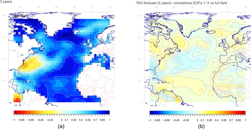
Part of the skill was associated with the long-term warming captured by the decadal forecasts based on the GFDL CM2.1 coupled ocean-atmosphere climate model. The question whether the skill was connected to the larger spatial scale anomalies was tested through an assessment where the forecasts were filtered through a set of leading EOFs: the first 20 EOFs were computed and then a subset of the leading modes were kept and used to reconstruct the forecasts. A subset of the three leading modes is presented in Fig. 4, but this assessment was also repeated with different subsets and with similar results (not shown). The leading EOF modes represented covariance patterns that usually involved larger spatial and temporal scales than the higher-order modes. A comparison between correlation scores for the filtered forecasts with the original forecasts against the NCAR/NCEP reanalysis suggests that there were regions with both higher and lower correlation scores (Fig. 4b). It was mainly in the central North Atlantic where small-scale variability seemed to reduce the correlation.

3.3.2. Ensemble members and common EOFs

We assessed the potential skill of the decadal forecasts in more detail by quantifying the spread of the different ensemble members in terms of the main modes of variability. A large spread would indicate less predictability than a smaller spread, and we used common EOFs to compare the ensemble members with the historical fields (see the Appendix). Hence, an additional assessment of skill involved a comparison between the PCs from the common EOFs, and the results indicated that there was a moderate spread among the ensemble members, suggesting that the forecasts were only moderately constrained by the known initial conditions and the boundary conditions (Fig. 5). In this analysis, we had combined temperature anomalies from the NCEP/NCAR reanalysis with corresponding temperature anomalies from the ten ensemble members from the decadal forecasts for corresponding times and spatial grid. The joint data matrix was then used to compute common EOFs in order to produce a set of spatial covariance patterns common for all and a set of PCs, which represented each of the data sets in the joint data matrix. Ten of the datasets were generated by the GCM while only one was from the reanalysis, and hence, the GCM results had a dominating influence on the leading spatial covariance pattern. All the curves showing the leading PC refer to the same spatial pattern (upper left panel), and the singular values suggested that this leading mode could account for almost 52% of the variance, which also indicated that the predicted spatial covariance structure was similar to that found in the reanalysis (see the Appendix for more on the common EOFs). The four leading EOFs could explain most of the total variance, suggesting that the model was able to produce anomalies with similar characteristics as those in the reanalysis data. The spatial structure associated with the common EOFs indicated that the strongest variability was in the Arctic near the edge of the sea-ice and that there was least action off the east coast of the USA, where the Gulf stream branches off the American continent and where the correlation between the ensemble mean forecast and the NCEP/NCAR reanalysis was the smallest (Fig. 4a). One explanation for the reduced skill in this region may be that the ocean model lacked sufficient spatial resolution to adequately represent the western boundary current, the separation of the Gulf Stream from the continent, and the ocean current meanders. It is also interesting to note that the decadal forecasts (red curves) predicted a similar long-term trend as the observations (black curve).

Fig. 5. Common EOFs estimated for the joint annual mean TAS NCEP/NCAR reanalysis and the forecasts. The upper left panel shows the common spatial anomaly structure common for the reanalysis and all ensemble members, the upper right shows the variance associated with each EOF (singular values) with cumulated variance (red), and the lower panel shows the PC where the black curve represents the reanalysis and the red curves indicate the ten ensemble members. The leading EOF accounted for more than 50% of the variance, and stood out as the most important mode. The PCs suggested that there was a weak-to-moderate scatter (with respect to the decadal variations) between the ensemble members, and hence some indication of predictive skill.

A similar assessment as for TAS was also carried out for the SLP results, and the results suggest that the atmospheric circulation patterns were less constrained by the ocean state compared to the TAS (Fig. 6a). Moreover, the spread between the ensemble members was more pronounced in the SLP than for TAS, which was evident from the common EOF results (Fig. 7). The leading EOF accounted for most of the variance both in SLP and TAS (Figs. 5 and 7), and for SLP, the spatial EOF pattern suggested that there was a linkage with the North Atlantic Oscillation (NAO). The NAO is well-known to be associated with pronounced variations in the winter-time precipitation and temperature over northern Europe, and may be influenced by a range of conditions including the stratosphere (Thompson et al., 2002; Cagnazzo and Manzini, 2009; Ripesi et al., 2012). On a longer timescale of nine years, the magnitude of the correlation was greater than for the three-year timescale (Fig. 6b), and one possible explanation may be that the reduced sample size of non-overlapping forecasts over the 1961–2011 interval results in more pronounced sampling fluctuations. Figure 6 suggests that there was no indication of improved skill with longer timescales for SLP. Having established that large scales were prominent for TAS but not for SLP, that there was a dependency between large and small scales in the historical observations, and that the decadal forecasts made with GFDL CM2.1 exhibited some skill for TAS but less so, for SLP, we now have a context for evaluating MOS applied to the decadal forecasts. We proceeded with applying MOS to the decadal forecasts.

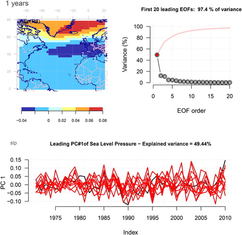
Fig. 6. (a) Same as Fig. 4a, but showing correlation maps for NCAR/NCEP reanalysis 1 and forecasted three-year mean SLP. The correlations were substantially lower than for TAS, suggesting less skillful forecasts when it comes to atmospheric circulation patterns. (b) Correlation maps for observed and forecasted nine-year mean SLP.

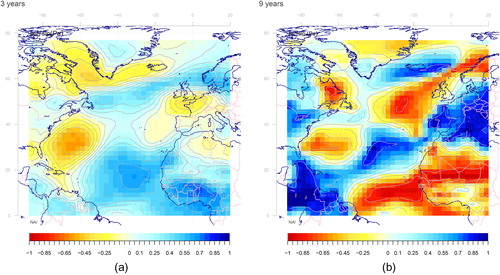
Fig. 7. Common EOFs estimated for the joint annual SLP NCEP/NCAR reanalysis and the forecasts. The upper left panel shows the common spatial anomaly structure common for the reanalysis and all ensemble members, the upper right shows the variance associated with each EOF (singular values) with cumulated variance (red), and the lower panel shows the PC where the black curve represents the reanalysis and the red curves indicate the ten ensemble members. The leading EOF accounted for about 50% of the variance, and stood out as the most important mode. There was a substantial spread in way the PC was captured by the ensemble members.

3.4. Evaluation of MOS

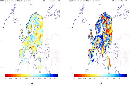
The added value of applying MOS to gridded precipitation statistics was tested through LOO cross-validation applied to the decadal forecast for both wet-day mean and frequency, but none of these predictions were associated with much skill. The lack of predictive skill in precipitation over Europe was also noted by Guemas et al. (2015). A correlation analysis between the ensemble mean of the LOO results for the wet-day frequency f_w and corresponding statistics from the gridded EOBS data returned scores scattered around zero (–0.02) for timescales of three years (Fig. 8a), but slightly higher for longer timescales (nine years: 0.14) (Fig. 8b). The same diagnostics for the wet-day mean μ showed similar mean correlation scores as for the wet-day frequency (Fig. 9). One possible reason for the poor prediction of the wet-day frequency may be that the forecasts of SLP were associated with pronounced ensemble spread, and a correlation analysis suggested little resemblance with the observed SLP field in terms of the NCEP/NCAR reanalysis 1 (Figs. 6 and 7).

Fig. 8. The correlation between (a) the three-year and (b) nine-year wet-day frequency estimated from the EOBS data and the mean MOS results taken over the entire ensemble. The results indicated low skill for the prediction of three-year f_w.

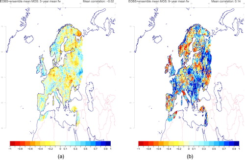
Fig. 9. The correlation between the (a) three-year and (b) nine-year wet-day mean precipitation estimated from the EOBS data and the mean MOS results taken over the entire ensemble. The correlations were more heterogeneous for μ than for f_w, with several regions that had higher values. However, there were also regions with weak scores.

In addition to using common EOFs to compare the raw decadal forecasts with the reanalysis data, they were also used to assess the MOS results against the observations, where common EOFs were calculated for the ensemble mean LOO results for μ and corresponding wet-day mean precipitation from the EOBS data (not shown). The PCs of the common EOFs suggested that both the decadal forecasts and the observations contained a long-term increasing trend, which can be associated with the past warming. For the wet-day frequency, the part of the leading PC representing the ensemble mean MOS results had significantly reduced variance compared to the observations, suggesting poor skills (R²; not shown).

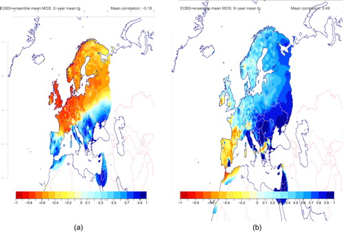
The annual mean temperature over Europe is influenced by the large-scale temperature structure over the North Atlantic, as demonstrated with LOO cross-validation for a downscaling exercise using NCEP/NCAR reanalysis 1 TAS (both maritime and continental) as predictor (Fig. 10), and the leading EOF for the annual temperature pattern accounted for 66% of the total variance in the EOBS data over Europe. The combination of spatial weights from the multiple regression in the ESD cross-validation exercise reproduced a similar spatial pattern (upper left panel) as the leading EOF of annual mean temperature from EOBS (upper left), and a correlation of 0.97 in the cross-validation indicated a strong link between the two (lower left). The MOS was repeated for the gridded annual mean of the daily mean temperature from the EOBS set. Two experiments were carried out, one where the predictor was taken to be the marine TAS over the North Atlantic and where the temperature over land was masked, and one using both maritime and continental temperatures. The first experiment, which included maritime temperatures, was expected to yield better scores only if the temperatures over the ocean are more predictable, as the temperature over land often has higher variance and is more strongly affected by circulation patterns. Hence, a MOS that uses maritime temperatures as predictors may enhance the skill for decadal predictions. However, the evaluation of the MOS for annual mean TAS forecasts indicated that there was low skill for three-year time scales over northern and western Europe where the correlation skill scores were negative (Fig. 11a). For time scales of 3–5 years, there was an enhancement of the correlation in the southern part of Europe (not shown), and for time scales around 9 years and greater, the correlation was high for most of Europe with a mean correlation of 0.49 (Fig. 11b). These skill scores reflected the long-term trend, which was reproduced in the decadal forecasts, and ephemeral variations over northern Europe with time scale <5 years and low predictive skill suggested that the shorter time scales were strongly influenced by SLP and the NAO.

Fig. 10. Results from the ESD experiment indicated a strong link between large-scale and local annual mean TAS anomalies. The upper left panel shows the pattern of the leading EOF estimated for the annual TAS from EOBS, upper right shows the TAS anomalies from the NCEP/NCAR reanalysis 1 associated with variations in the leading PC, lower left shows a scatter plot between the original PC and predictions in terms of LOO cross-validation, and the lower right shows the original time series (black) and the calibrated results (red).

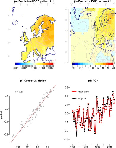
Fig. 11. The correlation between the (a) three-year and (b) nine-year mean TAS estimated from the EOBS data and the mean MOS results taken over the entire ensemble. The results indicated low skill for the prediction of three-year TAS. Only the maritime air temperatures from the decadal predictions were used to downscale the gridded temperature over Europe.

The analysis presented in Figs. 4–11 was repeated for forecasts for the annual, two-year means, four-year means, six-year means and so on up to nine-year aggregated value, and the skills varied gradually with time scale in accordance to the differences between the three/five/nine-year aggregates (not shown).

4. Discussion

The skill assessment here was different to the common strategy for decadal forecasts, which often involves a comparison between the skill of the initialised forecasts with that of the non-initialised forecasts. In this case, the comparison was made between aggregated statistics from short and long forecast intervals and corresponding intervals of observations because we were concerned with a question concerning scales as well as the merit of initialisation of the model simulations.

One reason for low predictive skill on decadal time scales over Europe was that the temperature and precipitation statistics were closely linked to the atmospheric circulation regime, and the large-scale SLP was only loosely constrained in terms of ocean heat distribution. Furthermore, the SLP was associated with shorter time scales and had a particularly strong link to the wet-day frequency, but also to the temperature. Here, the temperature and precipitation statistics were aggregated for all seasons, however, it is possible that there may be seasonal differences (Benestad and Mezghani, 2015).

One may question if it makes sense to assess whether MOS can add any value when it is already known that the GCM cannot predict large-scale circulation patterns of satisfying skill. In this case, we tried to distill more information from the ensemble than the traditional ensemble mean and emphasise the large-scale co-variance to get a better test. Furthermore, MOS can improve skill if the model systematically displaces phenomena in terms of their location but still manages to predict their timing, i.e. the activity of low pressure systems along the storm tracks or temperature anomalies connected to ocean currents. These results bring up another question about how much skill should a GCM have before downscaling can add more value. Trial and error provide steps towards learning more about these issues, and both successes and failures are important to report as a neglect to publish negative outcomes results in a publication bias (Joober et al., 2012; Mlinari et al., 2017). The lesson from this study was the importance of the atmospheric circulation and its degree of predictability on decadal scales. The most prominent large-scale SLP anomaly over the North Atlantic resembles the NAO pattern (Fig. 7), which has been notoriously difficult to forecast. It may be influenced by the position of the polar jet (Baldwin et al., 2007), the stratosphere (Thompson et al., 2002; Cagnazzo and Manzini, 2009; Ripesi et al., 2012), and the sea-ice extent (Petoukhov and Semenov, 2010; Orsolini et al., 2011; Francis and Vavrus, 2012), in addition to the North Atlantic SST, and it co-varies with the North Atlantic storm tracks. The large-scale maritime TAS over the North Atlantic, on the other hand, is more strongly constrained by the ocean state and its effect on the European mainland is mediated through atmospheric advection.

The analysis of the decadal forecasts presented here cannot support the hypothesis that MOS adds value in terms of making use of large-scale anomalies associated with higher predictive skills than local small-scale variations, although this does not rule out the possibility that MOS may enhance such forecasts in general. The GCM, on which these results were based, may not necessarily be representative of the best decadal forecasts or decadal forecasting in general. It is possible that better models exist with higher spatial resolution and better ability to represent the oceanic state and the ocean currents, and their influence on the overlying atmosphere. The Achilles heel of decadal forecasts seems to be connected to the atmospheric circulation, which in this GCM appeared to be less predictable. The GFDL-CM2.1 model simulates a motion within the atmosphere that is only weakly influenced by the underlying boundary conditions, such as heat sources, and this weak constraint limits the skill of decadal predictions over the continental Europe. There is also a region off the eastern coast of North America with low predictability where the Gulf current separates from the continent.

The scales in time and space appear to be related, but differ for TAS and SLP. Large-scale temperature anomalies are associated with longer time scales such as long-term trends; however, there are also some indications of variations with 20–30 year time scales. For SLP, on the other hand, the aggregation over space does not translate into longer time scales, but reduced variance. The SLP provides a measure of the air mass residing above the sea, and an average over a large area reflects the total mass within a segment of the atmosphere. The total air mass is not expected to change much over time; however, on smaller spatial scales, the air column is affected by atmospheric waves or temperatures at different heights. There is also little indication that large scales in terms of leading EOFs are associated with higher skills than small-scale variability (higher-order EOFs), and there is also a weak link between the saturation water vapour pressure, which is a function of TAS, and the wet-day mean precipitation. Both the TAS and the wet-day mean precipitation exhibit a long-term trend associated with the general warming, and the higher skill scores for μ predictions on longer time scales may partly be due to a common trend.

It is important to keep in mind that while different scales reflect different physical processes, the statistical character of aggregated data is also affected by the choice of time intervals and spatial representation, which also have an effect on the sample size. The standard error of the mean is $\sigma /\sqrt{n-1}$ (Barde and Barde, 2012) and the diminishing error with sample size may be one reason why it may be easier to detect a signal in longer intervals and over larger regions (Hibino and Takayabu, 2016). Hence, for the case of decadal forecasting, an improved skill can be expected both from emphasising the slow processes as well as the higher accuracy in estimating the mean value.

5. Conclusion

Decadal forecasts derived from a GCM were subject to MOS-based ESD over the North Atlantic and European region, but the analysis of skill suggested low predictability on three-year timescales, mainly due to the fact that the atmospheric circulation was weakly constrained by the oceanic state. Precipitation and temperature over Europe were strongly influenced by such circulation patterns, and in particular variability resembling the NAO and corresponding large-scale mean SLP anomalies. There was also little indication that large-scale anomalies were more predictable than small-scale variability according to these forecasts, hence undermining the assumption for MOS enhancing the predictive skill on decadal time scales. Higher skill was found for forecasts with longer timescale of nine years; however, the higher scores may have been partly inflated by common long-term warming trends.

Acknowledgements

We would like to acknowledge the teams who have produced the NCEP/NCAR reanalyses, the gridded EOBS data, and the GCM runs (FP7-SPECS). The NCEP Reanalysis data was provided by the NOAA/OAR/ESRL PSD, Boulder, Colorado, USA, from their Web site at http://www.esrl.noaa.gov/psd/ and we acknowledge the E-OBS dataset from the EU-FP6 project ENSEMBLES (http://ensembles-eu.metoffice.com) and the data providers in the ECA&D project (http://www.ecad.eu). We are also grateful for constructive comments from two anonymous reviewers.

Disclosure statement

No potential conflict of interest was reported by the authors.

Additional information

Funding

This work was funded under the FP7-SPECS (EU Grant Agreement 3038378). L.P.C. and F.J.D.R. were also supported by the H2020 EUCP (GA 776613) and the Spanish MINECO CLINSA (CGL2017-85791-R) and HIATUS (CGL2015-70353-R) projects.

Appendix

Method: a detailed description

Description of decadal forecasts

Our analysis relied on a 10-member GCM ensemble of 10-year long hindcasts based on GFDL CM2.1, initialised every year (either January 1st or November 1st) for the period 1961–2011 such as to bring the state of the coupled models close to observations and align the simulated natural variability with the observed variability. In other words, the raw decadal forecasts involved 51 × 10 forecasts. The GFDL CM2.1 horizontal atmospheric resolution was 2${}^{°}$ latitude × 2.5${}^{°}$ longitude while the ocean horizontal resolution was 1${}^{°}$ in latitude and longitude, with the meridional resolution equator-ward of 30 increasing progressively such as to reach $\sim {0.3}^{°}$ at the equator. The atmospheric component of the model had 24 vertical levels while the ocean component had 50 vertical levels, 22 of which were evenly spaced within the top 220 m.

All the simulations were performed by following the protocol established by the Coupled Model Intercomparison Project Phase 5 (CMIP5) project. Thus, the external forcing (greenhouse gases, solar activity, stratospheric aerosols associated with volcanic eruptions, and anthropogenic aerosols) were taken from observations for the period 1961–2005 and from the RCP 4.5 scenario (Representative Concentration Pathway 4.5 $\mathrm{W}/{\mathrm{m}}^2$; Meinshausen et al. (2011)) estimates from 2006 onward. It should be noted that some of these radiative forcings would not be known in a true prediction exercise, and as such, the results can be better understood as an upper limit on predictability.

The raw model output and the predictors

Here, a subset of the forecasts was evaluated as the combination of all possibilities would be too large for this paper. We analysed a set of different forecast intervals, which refer to the duration of the forecast: the first and last forecasted TAS or SLP. The predictors were TAS and SLP averaged over the forecast intervals, ranging from a year to 9 years of duration. Thus, for a forecast interval of one year, we used the annual mean, for a three-year-interval, we used the three-year-mean, and so on. The decadal forecasts were taken from the GFDL-CM2.1 GCM from the FP7-SPECS project with nine different forecasted lead times (0-8 years), each with 10 ensemble members. We only used forecasts with one year lead before the 1–9 year forecast period. Hence, only a limited time window t₁–t₂ was used from these simulations, and the predictor was taken as the mean aggregated over this time window and the forecasted quantity was derived according to $\overline{x(t)}, t\in [t_1, t_2]$.

The analysis

To avoid misunderstanding, the term ‘multivariate’ is used here to refer to a field consisting of many variables of the same type (either TAS or SLP, but not a combination of the two). Moreover, the analysis was applied to data matrices holding a set of either TAS or SLP observed or forecasted for different locations.

The predictands

The threshold value defining a wet day was set to 1 mm/day, and the precipitation parameters f_w and μ were estimated from the daily data sets through the use of CDO (https://code.mpimet.mpg.de/projects/cdo). The predictor for μ was the saturation vapour pressure estimated from the SAT as in Benestad and Mezghani (2015) ($e_s={10}^{(11.4-2353/T)}$, where T is the temperature in degrees Kelvin), whereas the predictor for f_w was the SLP. If the number of wet days is $n_w=\sum _t\mathcal{H}(x_t-x_0)$, where $\mathcal{H}$ is the Heaviside function, x_t is the precipitation recorded on day t, x₀ is the threshold (1 mm/day), and n_t is the total number of days, then the mathematical expression for the wet-day mean frequency is $f_w=n_w/n_t$ and the wet-day mean precipitation is $\mu =\sum _t{x}_t\mathcal{H}(x_t-x_0)/n_w$. Four EOFs were used to represent the predictands and the four leading EOFs for μ were associated with ∼14.0, 8.3, 7.4 and 5.5% (total 32.5%) of the variance and 18.5, 11.5, 7.2, 4.9% (total 42.1%) for f_w, respectively. For optimal results, a MOS would need to include enough EOFs to account for most of the covariance; however, since we were merely evaluating its potential, we limited our set to the four leading modes. The low variance for the modes higher than four suggested that there were no pronounced extensive and coherent spatial covariance patterns that typically can be connected to large-scale conditions. Moreover, the low fraction of the variance suggest that a significant part of the rainfall statistics has a more local character that is not represented here. For the annual daily mean EOBS temperature, the variance of the four leading EOFs accounted for 66.3, 10.4, 6.1 and 4.4% of the total variance, and combined, they accounted for 97.2%.).

Common EOFs

Spatio-temporal patterns in different data sources can be compared if the data is presented on a common grid and combined in one matrix. Both traditional EOF and common EOFs can be used in diagnostic analyses as well as providing a basis for prediction for multivariate datasets. The fundamental idea is that a data matrix X can be decomposed into orthogonal components, e.g. through the means of singular value decomposition $X=\mathit{UW}{V}^T$ (Press, 1989). In this case, U is a matrix holding the EOFs, V contains the PCs, W is a diagonal matrix containing singular values, and $U^{T}U=V^{T}V=I$. It is possible to combine a number of different data sets through concatenation along the time dimension, and then estimate EOFs for the combined data matrix. Such EOFs are known as common EOFs (Barnett, 1999), and were used here to represent the predictors in terms of all ensemble members, where the PCs contained information about the different ensemble members and the EOFs described spatial structures common to all.

Downscaling and MOS

A set of EOFs was derived from forecasts for all ensemble members from selected initialisations, lead time and aggregated over a forecast interval. The PCs associated with the EOFs were used in a stepwise multiple regression analysis (Benestad, 2001) against corresponding PCs representing the predictands. In most cases, the data matrix X used as input for the EOFs consisted of the ten ensemble members concatenated in time, however, in some cases where it was used for diagnostic, it was also applied to a data matrix consisting the ensemble mean value (the supporting material). For the former, the size of the data matrix was $n\times m\times S$ for n forecasts, an ensemble size of m = 10, and S is the number of grid-box values. As predictand, we used the either precipitation parameters (f_w or μ) or daily mean temperature from the EOBS, just as in the ESD exercises where the predictors were taken from the NCEP/NCAR reanalysis rather than the decadal forecasts themselves.

The ESD technique used to diagnose the connections between the scales in the historical data and to calibrate models for MOS used a stepwise multiple regression between the predictand y and a set of predictors $[x_1, x_2,\dots ]$ based on the simple linear equation $y={\beta }_0+\sum _i{\beta }_i{x}_i$ (for each predictand). Both the predictands and the predictors were taken to be the PCs that describe how the presences of the different EOF patterns vary from time to time. Here, we used an ordinary least squares model and the stepwise screening was based on the Akaike information criterion.

The MOS was applied to all ensemble members and observations, and the set of observations was repeated once for each ensemble member so that each member had a match in the observations. In order to ensure a proper synchronisation, the matching of data points relied on using the dates of the data; Each initialisation of forecasts was carried out for different years, and the dates corresponding to the first member was associated with YYYY-01-01 (YYYY being the year of the forecast), the second member YYYY-01-02, and so on. The repeated use of observations and including all ensemble members in the calibration gave a larger training sample than using single members or ensemble means. In addition, making use of the entire forecast ensemble in the calibration took advantage of more information embedded than just the ensemble mean, as large model spread affected the calibration of the MOS model and provided an indication of the model skill. Hence, R² from the regression analysis reflected the predictability of decadal variability.

LOO cross-validation

The MOS skill was assessed using a LOO cross-validation, which involved withholding one forecasting interval common for all members (Wilks, 1995). EOFs were estimated for the predictand based on the calibration set data, but the data matrix X excluded the interval used for the evaluation. The predictions for the independent evaluation sample corresponded to the PCs, which were associated with the EOFs from the calibration sample, but the end results were derived using these EOF products to recover the gridded field structure of the data. The use of EOFs was similar to using principal component analysis (PCA) for representing predictands, and was explored by Benestad et al. (2015a) who found that PCA-based downscaling gave more robust results and a marginal improvement in the cross-validation skills. This split before computing the predictand EOFs was not applied to the predictors, because the MOS would always make use of the full predictor field; Whereas the part of the predictors synchronised with the observations were used for the calibration, the other part was used for prediction. It was most convenient and simplest to compute EOFs for the entire field and use different segments of the PCs for the training and forecasting.

References

- Baldwin, M. P., Rhines, P. B., Huang, H.-P. and McIntyre, M. E. 2007. Atmospheres. The jet-stream conundrum. Science 315, 467–468. doi:10.1126/science.1131375
- Barde, M. P. and Barde, P. J. 2012. What to use to express the variability of data: standard deviation or standard error of mean? Perspect. Clin. Res. 3, 113–116. 4103/2229-3485.100662. URL https://www.ncbi.nlm.nih.gov/pmc/articles/PMC3487226/. doi:10.4103/2229-3485.100662
- Barnett, T. P. 1999. Comparison of near-surface air temperature variability in 11 coupled global climate models. J. Climate 12, 511–518. doi:10.1175/1520-0442(1999)012<0511:CONSAT>2.0.CO;2
- Benestad, R. 2007. Novel methods for inferring future changes in extreme rainfall over northern Europe. Clim. Res. 34, 195–210. doi:10.3354/cr00693
- Benestad, R., Sillmann, J., Thorarinsdottir, T. L., Guttorp, P., Mesquita, M. D. S. and co-authors. 2017. New vigour involving statisticians to overcome ensemble fatigue. Nat. Clim. Change 7, 697–703. URL http://www.nature.com/doifinder/10.1038/nclimate3393. doi:10.1038/nclimate3393
- Benestad, R. E. 2001. A comparison between two empirical downscaling strategies. Int. J. Climatol. 21, 1645–1668. doi:10.1002/joc.703
- Benestad, R. E., Chen, D., Mezghani, A., Fan, L. and Parding, K. 2015a. On using principal components to represent stations in empirical-statistical downscaling. Tellus A 67. v67.28326, URL http://www.tellusa.net/index.php/tellusa/article/view/28326.
- Benestad, R. E. and Mezghani, A. 2015. On downscaling probabilities for heavy 24-hour precipitation events at seasonal-to-decadal scales. Tellus A 67. doi:10.3402/tellusa.v67.25954, URL http://www.tellusa.net/index.php/tellusa/article/view/25954.
- Benestad, R. E., Mezghani, A. and Parding, K. M. 2015b. esd V1.0. doi:10.5281/zenodo.29385.
- Benestad, R. E., Parding, K. M., Isaksen, K. and Mezghani, A. 2016. Climate change and projections for the Barents region: what is expected to change and what will stay the same? Environ. Res. Lett. 11, 054017. URL http://stacks.iop.org/1748-9326/11/i=5/a=054017. doi:10.1088/1748-9326/11/5/054017
- Cagnazzo, C. and Manzini, E. 2009. Impact of the Stratosphere on the Winter Tropospheric Teleconnections between ENSO and the North Atlantic and European Region. J. Climate 22, 1223–1238. doi:10.1175/2008JCLI2549.1
- Caron, L.-P., Hermanson, L. and Doblas-Reyes, F. J. 2015. Multiannual forecasts of Atlantic U.S. tropical cyclone wind damage potential. Geophys. Res. Lett. 42, 2417–2425. doi:10.1002/2015GL063303
- Caron, L.-P., Jones, C. G. and Doblas-Reyes, F. 2014. Multi-year prediction skill of Atlantic hurricane activity in CMIP5 decadal hindcasts. Clim. Dyn. 42, 2675–2690. URL http://link.springer.com/10.1007/s00382-013-1773-1. doi:10.1007/s00382-013-1773-1
- Chang, E. K. M., Guo, Y. and Xia, X. 2012. CMIP5 multimodel ensemble projection of storm track change under global warming. J. Geophys. Res. 117. doi:10.1029/2012JD018578. URL http://doi.wiley.com/10.1029/2012JD018578.
- Chikamoto, Y., Timmermann, A., Luo, J.-J., Mochizuki, T., Kimoto, M. and co-authors. 2015. Skilful multi-year predictions of tropical trans-basin climate variability. Nat. Commun. 6, 6869. URL doi:10.1038/ncomms7869
- Delworth, T. L., Broccoli, A. J., Rosati, A., Stouffer, R. J., Balaji, V. and co-authors. 2006. GFDL’s CM2 global coupled climate models - Part 1: formulation and simulation characteristics. J. Climate 19, 643–674. doi:10.1175/JCLI3629.1
- Doblas-Reyes, F. J., Andreu-Burillo, I., Chikamoto, Y., García-Serrano, J., Guemas, V. and co-authors. 2013. Initialized near-term regional climate change prediction. Nat. Commun. 4, 1715. URL http://www.pubmedcentral.nih.gov/articlerender.fcgi?artid=3644073&tool=pmcentrez&rendertype=abstract. doi:10.1038/ncomms2704
- Francis, J. A. and Vavrus, S. J. 2012. Evidence linking Arctic amplification to extreme weather in mid-latitudes. Geophys. Res. Lett. 39.
- Garca-Serrano, J., Doblas-Reyes, F. J. and Coelho, C. A S. 2012. Understanding Atlantic multi-decadal variability prediction skill. Geophys. Res. Lett. 39, L18708. 1029/2012GL053283, URL http://doi.wiley.com/10.1029/2012GL053283.
- Garca-Serrano, J., Guemas, V. and Doblas-Reyes, F. J. 2015. Added-value from initialization in predictions of Atlantic multi-decadal variability. Clim. Dyn. 44, 2539–2555. doi:10.1007/s00382-014-2370-7
- Guemas, V., Corti, S., García-Serrano, J., Doblas-Reyes, F. J., Balmaseda, M. and co-authors. 2013. The Indian Ocean: the region of highest skill worldwide in decadal climate prediction*. J. Climate 26, 726–739. URL http://journals.ametsoc.org/doi/abs/10.1175/JCLI-D-12-00049.1. doi:10.1175/JCLI-D-12-00049.1
- Guemas, V., García-Serrano, J., Mariotti, A., Doblas-Reyes, F. and Caron, L.-P. 2015. Prospects for decadal climate prediction in the Mediterranean region. QJR. Meteorol. Soc. 141, 580–597. URL http://doi.wiley.com/10.1002/qj.2379. doi:10.1002/qj.2379
- Hawkins, E. and Sutton, R. 2009. The potential to narrow uncertainty in regional climate predictions. Bull. Am. Meteor. Soc. 90, 1095. doi:10.1175/2009BAMS2607.1
- Hibino, K. and Takayabu, I. 2016. A trade-off relation between temporal and spatial averaging scales on future precipitation assessment. J. Meteor. Soc. Jpn. 94A, 121–134. URL https://www.jstage.jst.go.jp/article/jmsj/94A/0/94A_2015-056/_article. doi:10.2151/jmsj.2015-056
- Joober, R., Schmitz, N., Annable, L. and Boksa, P. 2012. Publication bias: what are the challenges and can they be overcome? J. Psychiatry Neurosci. 37, 149–152. URL https://www.ncbi.nlm.nih.gov/pmc/articles/PMC3341407/. doi:10.1503/jpn.120065
- Kalnay, E., Kanamitsu, M., Kistler, R., Collins, W., Deaven, D. and co-authors. 1996. The NCEP/NCAR 40-Year Reanalysis Project. Bull. Am. Meteor. Soc. 77, 437–471. doi:10.1175/1520-0477(1996)077<0437:TNYRP>2.0.CO;2
- Kharin, V. V., Boer, G. J., Merryfield, W. J., Scinocca, J. F. and Lee, W. S. 2012. Statistical adjustment of decadal predictions in a changing climate. Geophys. Res. Lett. 39, n/a–6. doi:10.1029/2012GL052647
- Kirtman, B., Power, S. B., Adedoyin, A. J., Boer, G. J., Bojariu, R. and co-authors 2013. Chapter 11 - Near-term climate change: projections and predictability. Climate Change 2013: The Physical Science Basis. IPCC Working Group I Contribution to AR5, IPCC. Cambridge University Press, Cambridge. URL http://www.climatechange2013.org/images/report/WG1AR5_Chapter11_FINAL.pdf.
- Linden, P. V. D. and J. F. B. Mitchell, Eds. 2009. Ensembles: climate change and its impacts: summary of Research and Results from the ENSEMBLES Project. European Comission, Met Office Hadley Centre, Exeter EX1 3PB, UK.
- Meehl, G. A., Goddard, L., Boer, G., Burgman, R., Branstator, G. and co-authors. 2014. Decadal climate prediction: an update from the trenches. Bull. Am. Meteor. Soc. 95, 243–267. 1, URL http://journals.ametsoc.org/doi/abs/10.1175/BAMS-D-12-00241.1. doi:10.1175/BAMS-D-12-00241.1
- Meinshausen, M., Smith, S. J., Calvin, K., Daniel, J. S., Kainuma, M. L. T. and co-authors. 2011. The RCP greenhouse gas concentrations and their extensions from 1765 to 2300. Climatic Change 109, 213–241. URL http://link.springer.com/10.1007/s10584-011-0156-z. doi:10.1007/s10584-011-0156-z
- Mlinari, A., Horvat, M. and Upak Smoli, V. 2017. Dealing with the positive publication bias: why you should really publish your negative results. Biochem. Med. 27, 030201. URL https://www.ncbi.nlm.nih.gov/pmc/articles/PMC5696751/. doi:10.11613/BM.2017.030201
- Mochizuki, T., Ishii, M., Kimoto, M., Chikamoto, Y., Watanabe, M. and co-authors. 2010. Pacific decadal oscillation hindcasts relevant to near-term climate prediction. Proc. Natl. Acad. Sci. U.S.A 107, 1833–1837. URL http://www.pubmedcentral.nih.gov/articlerender.fcgi?artid=2804740&tool=pmcentrez&rendertype=abstract. doi:10.1073/pnas.0906531107
- Neu, U. 2012. IMILAST a community effort to intercompare extratropical cyclone detection and tracking algorithms: assessing method-related uncertainties. Bull. Am. Meteor. Soc. 120919072158001. URL http://journals.ametsoc.org/doi/abs/10.1175/BAMS-D-11-00154.1.
- Orsolini, Y., Senan, R., Benestad, R. E. and Melsom, A. 2011. Autumn atmospheric response to the 2007 low Arctic sea ice extent in coupled ocean-atmosphere hindcasts. Clim. Dyn. 38, 2437–2448.
- Petoukhov, V. and Semenov, V. A. 2010. A link between reduced Barents-Kara sea ice and cold winter extremes over northern continents. J. Geophys. Res. 115.
- Press, W. H., Ed. 1989. Numerical Recipes in Pascal: The Art of Scientific Computing. Cambridge University Press, Cambridge.
- Ripesi, P., Ciciulla, F., Maimone, F. and Pelino, V. 2012. The February 2010 Arctic Oscillation Index and its stratospheric connection. QJR Meteorol. Soc. 138, 1961–1969. URL http://doi.wiley.com/10.1002/qj.1935. doi:10.1002/qj.1935
- Robson, J., Sutton, R. and Smith, D. 2014. Decadal predictions of the cooling and freshening of the North Atlantic in the 1960s and the role of ocean circulation. Clim. Dyn. 42, 2353–2365. URL http://link.springer.com/10.1007/s00382-014-2115-7. doi:10.1007/s00382-014-2115-7
- Smith, D. M., Scaife, A. A., Boer, G. J., Caian, M., Doblas-Reyes, F. J. and co-authors. 2013. Real-time multi-model decadal climate predictions. Clim. Dyn. 41, 2875–2888. URL http://link.springer.com/10.1007/s00382-012-1600-0. doi:10.1007/s00382-012-1600-0
- Sutton, R. and Allen, M. 1997. Decadal predictability of North Atlantic sea surface temperature and climate. Nature 388, 563–567. doi:10.1038/41523
- Takayabu, I., Kanamaru, H., Dairaku, K., Benestad, R., Storch, H. V. and Christensen, J. H. 2016. Reconsidering the quality and utility of downscaling. J. Meteorol. Soc. Jpn. 94A, 31–45. doi:10.2151/jmsj.2015-042
- Thompson, D. W. J., Baldwin, M. P. and Wallace, J. M. 2002. Stratospheric connection to northern hemisphere wintertime weather: implications for prediction. J. Climate 15, 1421–1428. doi:10.1175/1520-0442(2002)015<1421:SCTNHW>2.0.CO;2
- Wilks, D. S. 1995. Statistical Methods in the Atmospheric Sciences. Academic Press, Orlando, Florida, USA.