Improving the condition number of estimated covariance matrices

Abstract

High dimensional error covariance matrices and their inverses are used to weight the contribution of observation and background information in data assimilation procedures. As observation error covariance matrices are often obtained by sampling methods, estimates are often degenerate or ill-conditioned, making it impossible to invert an observation error covariance matrix without the use of techniques to reduce its condition number. In this paper, we present new theory for two existing methods that can be used to ‘recondition’ any covariance matrix: ridge regression and the minimum eigenvalue method. We compare these methods with multiplicative variance inflation, which cannot alter the condition number of a matrix, but is often used to account for neglected correlation information. We investigate the impact of reconditioning on variances and correlations of a general covariance matrix in both a theoretical and practical setting. Improved theoretical understanding provides guidance to users regarding method selection, and choice of target condition number. The new theory shows that, for the same target condition number, both methods increase variances compared to the original matrix, with larger increases for ridge regression than the minimum eigenvalue method. We prove that the ridge regression method strictly decreases the absolute value of off-diagonal correlations. Theoretical comparison of the impact of reconditioning and multiplicative variance inflation on the data assimilation objective function shows that variance inflation alters information across all scales uniformly, whereas reconditioning has a larger effect on scales corresponding to smaller eigenvalues. We then consider two examples: a general correlation function, and an observation error covariance matrix arising from interchannel correlations. The minimum eigenvalue method results in smaller overall changes to the correlation matrix than ridge regression but can increase off-diagonal correlations. Data assimilation experiments reveal that reconditioning corrects spurious noise in the analysis but underestimates the true signal compared to multiplicative variance inflation.

Keywords:

• condition number
• covariance approximation
• observation error covariance matrix
• data assimilation
• reconditioning

1. Introduction

The estimation of covariance matrices for large dimensional problems is of growing interest (Pourahmadi, 2013), particularly for the field of numerical weather prediction (NWP) (Weston et al., 2014; Bormann et al., 2016) where error covariance estimates are used as weighting matrices in data assimilation problems (e.g. Ghil, 1989; Daley, 1991; Ghil and Malanotte-Rizzoli, 1991). At operational NWP centres there are typically $\mathcal{O}({10}^7)$ measurements every 6 h (Bannister, 2017), meaning that observation error covariance matrices are extremely high-dimensional. In nonlinear least-squares problems arising in variational data assimilation, the inverses of correlation matrices are used, meaning that well-conditioned matrices are vital for practical applications (Bannister, 2017). This is true in both the unpreconditioned and preconditioned variational data assimilation problem using the control variable transform, as the inverse of the observation error covariance matrix appears in both formulations. The convergence of the data assimilation problem can be poor if either the background or observation variance is small; however, the condition number and eigenvalues of background and observation error covariance matrices have also been shown to be important for convergence in both the unpreconditioned and preconditioned case in Haben et al. (2011a, 2011b), Haben (2011), Tabeart et al. (2018). Furthermore, the conditioning and solution of the data assimilation system can be affected by complex interactions between the background and observation error covariance matrices and the observation operator (Johnson et al., 2005; Tabeart et al., 2018). The condition number of a matrix, $\mathbf{A},$ provides a measure of the sensitivity of the solution $\mathbf{x}$ of the system $\mathbf{Ax}=\mathbf{b}$ to perturbations in $\mathbf{b}.$ The need for well-conditioned background and observation error covariance matrices motivates the use of ‘reconditioning’ methods, which are used to reduce the condition number of a given matrix.

In NWP applications, observation error covariance matrices are often constructed from a limited number of samples (Cordoba et al., 2016; Waller, Ballard, et al., 2016; Waller, Simonin, et al., 2016). This can lead to problems with sampling error, which manifest in sample covariance matrices, or other covariance matrix estimates, that are very ill-conditioned or can fail to satisfy required properties of covariance matrices (such as symmetry and positive semi-definiteness) (Ledoit and Wolf, 2004; Higham et al., 2016). In some situations, it may be possible to determine which properties of the covariance matrix are well estimated. One such instance is presented in Skøien and Blöschl (2006), which considers how well we can expect the mean, variance and correlation lengthscale of a sample correlation to represent the true correlation matrix depending on different properties of the measured domain (e.g. sample spacing, area measured by each observation). However, this applies only to direct estimation of correlations and will not apply to diagnostic methods (e.g. Desroziers et al., 2005), where transformed samples are used and covariance estimates may be poor. We note that in this paper, we assume that the estimated covariance matrices used in our experiments represent the desired correlation information matrix well and that differences are due to noise rather than neglected sources of uncertainty. This may not be the case for practical situations, where reconditioning may need to be performed in conjunction with other techniques to compensate for the underestimation of some sources of error.

Depending on the application, a variety of methods have been used to combat the problem of rank deficiency of sample covariance matrices. In the case of spatially correlated errors, it may be possible to fit a smooth correlation function or operator to the sample covariance matrix as was done in Simonin et al. (2019) and Guillet et al. (2019), respectively. Another approach is to retain only the first k leading eigenvectors of the estimated correlation matrix and to add a diagonal matrix to ensure the resulting covariance matrix has full rank (Stewart et al., 2013; Michel, 2018). However, this has been shown to introduce noise at large scales for spatial correlations and may be expensive in terms of memory and computational efficiency (Michel, 2018). Although localisation can be used to remove spurious correlations, and can also be used to increase the rank of a degenerate correlation matrix (Hamill et al., 2001), it struggles to reduce the condition number of a matrix without destroying off-diagonal correlation information (Smith et al., 2018). A further way to increase the rank of a matrix is by considering a subset of columns of the original matrix that are linearly independent. This corresponds to using a subset of observations, which is contrary to a key motivation for using correlated observation error statistics: the ability to include a larger number of observations in the assimilation system (Janjić et al., 2018). Finally, the use of transformed observations may result in independent observation errors (Migliorini, 2012; Prates et al., 2016); however, problems with conditioning will manifest in other components of the data assimilation algorithm, typically the observation operator. Therefore, although other techniques to tackle the problem of ill-conditioning exist, they each have limitations. This suggests that for many applications the use of reconditioning methods, which we will show are inexpensive to implement and are not limited to spatial correlations, may be beneficial.

We note that small eigenvalues of the observation error covariance matrix are not the only reason for slow convergence: if observation error standard deviations are small, the observation error covariance matrix may be well-conditioned, but convergence of the minimisation problem is likely to be poor (Haben, 2011; Tabeart et al., 2018). In this case reconditioning may not improve convergence and performance of the data assimilation routine.

Two methods, in particular, referred to in this work as the minimum eigenvalue method and ridge regression, are commonly used at NWP centres. Both methods are used by Weston (2011), where they are tested numerically. Additionally, in Campbell et al. (2017), a comparison between these methods is made experimentally and it is shown that reconditioning improves convergence of a dual four-dimensional variational assimilation system. However, up to now there has been minimal theoretical investigation into the effects of these methods on the covariance matrices. In this paper, we develop theory that shows how variances and correlations are altered by the application of reconditioning methods to a covariance matrix.

Typically reconditioning is applied to improve convergence of a data assimilation system by reducing the condition number of a matrix. However, the convergence of a data assimilation system can also be improved using multiplicative variance inflation, a commonly used method at NWP centres such as ECMWF (Liu and Rabier, 2003; McNally et al., 2006; Bormann et al., 2015, 2016) to account for neglected error correlations or to address deficiencies in the estimated error statistics by increasing the uncertainty in observations. It is not a method of reconditioning when a constant inflation factor is used, as it cannot change the condition number of a covariance matrix. In practice, multiplicative variance inflation is often combined with other techniques, such as neglecting off-diagonal error correlations, which do alter the conditioning of the observation error covariance matrix.

Although it is not a reconditioning technique, in Bormann et al. (2015) multiplicative variance inflation was found to yield faster convergence of a data assimilation procedure than either the ridge regression or minimum eigenvalue methods of reconditioning. This finding is likely to be system-dependent; the original diagnosed error covariance matrix in the ECMWF system has a smaller condition number than the corresponding matrix for the same instrument in the Met Office system (Weston et al., 2014). Additionally, in the ECMWF system, the use of reconditioning methods only results in small improvements to convergence, and there is little difference in convergence speed for the two methods. This contrasts with the findings of Weston (2011), Weston et al. (2014), and Campbell et al. (2017) where differences in convergence speed when using each method of reconditioning were found to be large. Therefore, it is likely that the importance of reducing the condition number of the observation error covariance matrix compared to inflating variances will be sensitive to the data assimilation system of interest. Aspects of the data assimilation system that may be important in determining the level of this sensitivity include: the choice of preconditioning and minimisation scheme (Bormann et al., 2015), quality of the covariance estimate, interaction between background and estimated observation error covariance matrices within the data assimilation system (Fowler et al., 2018; Tabeart et al., 2018), the use of thinning and different observation networks. We also note that Stewart et al. (2009, 2013) and Stewart (2010) consider changes to the information content and analysis accuracy corresponding to different approximations to a correlated observation error covariance matrix (including an inflated diagonal matrix). Stewart et al. (2013) and Healy and White (2005) also provide evidence in idealized cases to show that inclusion of even approximate correlation structure gives significant benefit over diagonal matrix approximations, including when variance inflation is used.

In this work, we investigate the minimum eigenvalue and ridge regression methods of reconditioning as well as multiplicative variance inflation, and analyse their impact on the covariance matrix. We compare both methods theoretically for the first time, by considering the impact of reconditioning on the correlations and variances of the covariance matrix. We also study how each method alters the objective function when applied to the observation error covariance matrix. Other methods of reconditioning, including thresholding (Bickel and Levina, 2008) and localisation (Horn and Johnson, 1991; Ménétrier et al., 2015; Smith et al., 2018) have been discussed from a theoretical perspective in the literature but will not be included in this work. In Section 2, we describe the methods more formally than in previous literature before developing new related theory in detail in Section 3. We show that the ridge regression method increases the variances and decreases the correlations for a general covariance matrix and the minimum eigenvalue method increases variances. We prove that the increases to the variance are bigger for the ridge regression method than the minimum eigenvalue method for any covariance matrix. We show that both methods of reconditioning reduce the weight on observation information in the objective function in a scale-dependent way, with the largest reductions in weight corresponding to the smallest eigenvalues of the original observation error covariance matrix. In contrast, multiplicative variance inflation using a constant inflation factor reduces the weight on observation information by a constant amount for all scales. In Section 4, the methods are illustrated via numerical experiments for two types of covariance structures. One of these is a simple general correlation function, and one is an interchannel covariance arising from a satellite-based instrument with observations used in NWP. We provide physical interpretation of how each method alters the covariance matrix, and use this to provide guidance on which method of reconditioning is most appropriate for a given application. We present an illustration of how all three methods alter the analysis of a data assimilation problem, and relate this to the theoretical conclusions concerning the objective function. We finally present our conclusions in Section 5. The methods are very general and, although their initial application was to observation error covariances arising from NWP, the results presented here apply to any sampled covariance matrix, such as those arising in finance (Higham, 2002; Qi and Sun, 2010) and neuroscience (Schiff, 2011; Nakamura and Potthast, 2015).

2. Covariance matrix modification methods

We begin by defining the condition number. The condition number provides a measure of how sensitive the solution $\mathbf{x}$ of a linear equation $\mathbf{Ax}=\mathbf{b}$ is to perturbations in the data $\mathbf{b}.$ A ‘well-conditioned problem’ will result in small perturbations to the solution with small changes to $\mathbf{b},$ whereas for an ‘ill-conditioned problem’, small perturbations to $\mathbf{b}$ can result in large changes to the solution. Noting that all covariance matrices are positive semi-definite by definition, we distinguish between the two cases of strictly positive definite covariance matrices and covariance matrices with zero minimum eigenvalue. Symmetric positive definite matrices admit a definition for the condition number in terms of their maximum and minimum eigenvalues. For the remainder of the work, we define the eigenvalues of a symmetric positive semi-definite matrix $\mathbf{S}\in {\mathbb{R}}^{d\times d}$ via: (1) $${\lambda }_1(\mathbf{S})\ge \dots \ge {\lambda }_d(\mathbf{S})\ge 0.$$(1)

Theorem 1.

If $\mathbf{S}\in {\mathbb{R}}^{d\times d}$ is a symmetric positive definite matrix with eigenvalues defined as in (1) we can write the condition number in the L₂ norm as $\kappa (\mathbf{S})=\frac{{\lambda }_1(\mathbf{S})}{{\lambda }_d(\mathbf{S})}.$

Proof.

See Golub and Van Loan (1996, Sec. 2.7.2). □

For a singular covariance matrix, $\mathbf{S},$ the convention is to take $\kappa (\mathbf{S})=\infty$ (Trefethen and Bau, 1997, Sec. 12). We also note that real symmetric matrices admit orthogonal eigenvectors which can be normalised to produce a set of orthonormal eigenvectors.

Let $\mathbf{R}\in {\mathbb{R}}^{d\times d}$ be a positive semi-definite covariance matrix with condition number $\kappa (\mathbf{R})=\kappa .$ We wish to recondition $\mathbf{R}$ to obtain a covariance matrix with condition number κ_max (2) $$1\le {\kappa }_{\mathit{max}}<\kappa ,$$(2) where the value of κ_max is chosen by the user. We denote the eigendecomposition of $\mathbf{R}$ by (3) $$\mathbf{R}={\mathbf{V}}_{\mathbf{R}}\mathbf{\Lambda }{\mathbf{V}}_{\mathbf{R}}^T$$(3) where $\mathbf{\Lambda }\in {\mathbb{R}}^{d\times d}$ is the diagonal matrix of eigenvalues of $\mathbf{R}$ and ${\mathbf{V}}_{\mathbf{R}}\in {\mathbb{R}}^{d\times d}$ is a corresponding matrix of orthonormal eigenvectors.

In addition to considering how the covariance matrix itself changes with reconditioning, it is also of interest to consider how the related correlations and standard deviations are altered. We decompose $\mathbf{R}$ as $\mathbf{R}=\mathbf{\Sigma }\mathbf{C}\mathbf{\Sigma },$ where $\mathbf{C}$ is a correlation matrix, and $\mathbf{\Sigma }$ is a non-singular diagonal matrix of standard deviations. We calculate $\mathbf{C}$ and $\mathbf{\Sigma }$ via: (4) $$\mathbf{\Sigma }(i,i)=\sqrt{\mathbf{R}(i,i)},\hspace{1em}\mathbf{C}(i,j)=\frac{\mathbf{R}(i,j)}{\sqrt{\mathbf{R}(i,i)}\sqrt{\mathbf{R}(j,j)}}.$$(4)

We now introduce the ridge regression method and the minimum eigenvalue method, the two methods of reconditioning that will be discussed in this work. We then define multiplicative variance inflation. This last method is not a method of reconditioning, but will be used for comparison purposes with the ridge regression and minimum eigenvalues methods.

2.1. Ridge regression method

The ridge regression method (RR) adds a scalar multiple of the identity to $\mathbf{R}$ to obtain the reconditioned matrix ${\mathbf{R}}_{RR}.$ The scalar δ is set using the following method.

• Define $\delta =\frac{{\lambda }_1(\mathbf{R})-{\lambda }_d(\mathbf{R}){\kappa }_{\mathit{max}}}{{\kappa }_{\mathit{max}}-1}.$

• Set ${\mathbf{R}}_{RR}=\mathbf{R}+\delta \mathbf{I}$

We note that this choice of δ yields $\kappa ({\mathbf{R}}_{RR})={\kappa }_{\mathit{max}}.$

In the literature (Hoerl and Kennard, 1970; Ledoit and Wolf, 2004), ‘ridge regression’ is a method used to regularise least squares problems. In this context, ridge regression can be shown to be equivalent to Tikhonov regularisation (Hansen, 1998). However, in this paper, we apply ridge regression as a reconditioning method directly to a covariance matrix. For observation error covariance matrices, the reconditioned matrix is then inverted prior to its use as a weighting matrix in the data assimilation objective function. As we are only applying the reconditioning to a single component matrix in the variational formulation, the implementation of the ridge regression method used in this paper is not equivalent to Tikhonov regularisation applied to the variational data assimilation problem (Budd et al., 2011; Moodey et al., 2013). This is shown in Section 3.5 where we consider how applying ridge regression to the observation error covariance matrix affects the variational data assimilation objective function. The ridge regression method is used at the Met Office (Weston et al., 2014).

2.2. Minimum eigenvalue method

The minimum eigenvalue method (ME) fixes a threshold, T, below which all eigenvalues of the reconditioned matrix, ${\mathbf{R}}_{ME},$ are set equal to the threshold value. The value of the threshold is set using the following method.

• Set ${\lambda }_1({\mathbf{R}}_{ME})={\lambda }_1(\mathbf{R})$

• Define $T={\lambda }_1(\mathbf{R})/{\kappa }_{\mathit{max}}>{\lambda }_d(\mathbf{R}),$ where κ_max is defined in (2(2) $$1\le {\kappa }_{\mathit{max}}<\kappa ,$$(2) ).

• Set the remaining eigenvalues of ${\mathbf{R}}_{ME}$ via (5) $${\lambda }_k({\mathbf{R}}_{ME})=\{\begin{array}{cc}{\lambda }_k(\mathbf{R})\hfill & \text{if}{\lambda }_k(\mathbf{R})>T\hfill \\ T\hfill & \text{if}{\lambda }_k(\mathbf{R})\le T\hfill \end{array}.$$(5)

• Construct the reconditioned matrix via ${\mathbf{R}}_{ME}={\mathbf{V}}_{\mathbf{R}}{\mathbf{\Lambda }}_{ME}{\mathbf{V}}_{\mathbf{R}}^T,$ where ${\mathbf{\Lambda }}_{ME}(i,i)={\lambda }_i({\mathbf{R}}_{ME}).$

This yields $\kappa ({\mathbf{R}}_{ME})={\kappa }_{\mathit{max}}.$ The updated matrix of eigenvalues can be written as ${\mathbf{\Lambda }}_{ME}=\mathbf{\Lambda }+\mathbf{\Gamma },$ the sum of the original matrix of eigenvalues and $\mathbf{\Gamma },$ a low-rank diagonal matrix update with entries $\mathbf{\Gamma }(k,k)=\max \{T-{\lambda }_k,0\}.$ Using (3(3) $$\mathbf{R}={\mathbf{V}}_{\mathbf{R}}\mathbf{\Lambda }{\mathbf{V}}_{\mathbf{R}}^T$$(3) ) the reconditioned ${\mathbf{R}}_{ME}$ can then be written as: (6) $${\mathbf{R}}_{ME}={\mathbf{V}}_{\mathbf{R}}(\mathbf{\Lambda }+\mathbf{\Gamma }){\mathbf{V}}_{\mathbf{R}}^T=\mathbf{R}+{\mathbf{V}}_{\mathbf{R}}\mathbf{\Gamma }{\mathbf{V}}_{\mathbf{R}}^T.$$(6)

Under the condition that ${\kappa }_{\mathit{max}}>d-l+1,$ where l is the index such that ${\lambda }_l\le T<{\lambda }_{l-1},$ the minimum eigenvalue method is equivalent to minimising the difference $\mathbf{R}-{\mathbf{R}}_{ME}\in {\mathbb{R}}^{d\times d}$ with respect to the Ky-Fan 1-d norm (the proof is provided in Appendix). The Ky-Fan p – k norm (also referred to as the trace norm) is defined in Fan (1959) and Horn and Johnson (1991), and is used in Tanaka and Nakata (2014) to find the closest positive definite matrix with condition number smaller than a given constant. A variant of the minimum eigenvalue method is applied to observation error covariance matrices at the European Centre for Medium-Range Weather Forecasts (ECMWF) (Bormann et al., 2016).

2.3. Multiplicative variance inflation

Multiplicative variance inflation (MVI) is a method that increases the variances corresponding to a covariance matrix. Its primary use is to account for neglected error correlation information, particularly in the case where diagonal covariance matrices are being used even though non-zero correlations exist in practice. However, this method can also be applied to non-diagonal covariance matrices.

Definition 1.

Let $\alpha >0$ be a given variance inflation factor and $$\mathbf{R}=\mathbf{\Sigma }\mathbf{C}\mathbf{\Sigma }$$ be the estimated covariance matrix. Then multiplicative variance inflation is defined by (7) $${\mathbf{\Sigma }}_{\mathit{MVI}}=\alpha \mathbf{\Sigma }.$$(7)

This is equivalent to multiplying the estimated covariance matrix by a constant. The updated covariance matrix is given by (8) $${\mathbf{R}}_{\mathit{MVI}}=\left(\alpha \mathbf{\Sigma }\right)\mathbf{C}\left(\alpha \mathbf{\Sigma }\right)={\alpha }^2\mathbf{\Sigma }\mathbf{C}\mathbf{\Sigma }={\alpha }^2\mathbf{R}.$$(8) The estimated covariance matrix is therefore multiplied by the square of the inflation constant. We note that the correlation matrix, $\mathbf{C}$, is unchanged by application of multiplicative variance inflation.

Multiplicative variance inflation is used at NWP centres including ECMWF (Bormann et al., 2016) to counteract deficiencies in estimated error statistics, such as underestimated or neglected sources of error. Inflation factors are tuned to achieve improved analysis or forecast performance, and are hence strongly dependent on the specific data assimilation system of interest. Aspects of the system that might influence the choice of inflation factor include observation type, known limitations of the covariance estimate, and observation sampling or thinning.

Although variance inflation is not a method of reconditioning, as it is not able to alter the condition number of a covariance matrix, we include it in this paper for comparison purposes. This means that variance inflation can only be used in the case that the estimated matrix can be inverted directly, i.e. is full rank. Multiplicative variance inflation could also refer to the case where the constant inflation factor is replaced with a diagonal matrix of inflation factors. In this case, the condition number of the altered covariance matrix would change. An example of a study where multiple inflation factors are used is given by Heilliette and Garand (2015), where the meteorological variable to which an observation is sensitive determines the choice of inflation factor. However, this is not commonly used in practice, and will not be considered in this paper.

3. Theoretical considerations

In this section, we develop new theory for each method. We are particularly interested in the changes made to $\mathbf{C}$ and $\mathbf{\Sigma }$ for each case. Increased understanding of the effect of each method may allow users to adapt or extend these methods, or determine which is the better choice for practical applications.

We now introduce an assumption that will be used in the theory that follows.

Main Assumption: Let $\mathbf{R}\in {\mathbb{R}}^{d\times d}$ be a symmetric positive semi-definite matrix with ${\lambda }_1(\mathbf{R})>{\lambda }_d(\mathbf{R}).$

We remark that any symmetric, positive semi-definite matrix with ${\lambda }_1={\lambda }_d$ is a scalar multiple of the identity, and cannot be reconditioned since it is already at its minimum possible value of unity. Hence in what follows, we will consider only matrices $\mathbf{R}$ that satisfy the Main Assumption.

3.1. Ridge regression method

We begin by discussing the theory of RR. In particular, we prove that applying this method for any positive scalar, δ, results in a decreased condition number for any choice of $\mathbf{R}.$

Theorem 2.

Under the conditions of the Main Assumption, adding any positive increment to the diagonal elements of $\mathbf{R}$ decreases its condition number.

Proof.

We recall that ${\mathbf{R}}_{RR}=\mathbf{R}+\delta \mathbf{I}.$ The condition number of ${\mathbf{R}}_{RR}$ is given by (9) $$\kappa ({\mathbf{R}}_{RR})=\frac{{\lambda }_1({\mathbf{R}}_{RR})}{{\lambda }_d({\mathbf{R}}_{RR})}=\frac{{\lambda }_1(\mathbf{R})+\delta }{{\lambda }_d(\mathbf{R})+\delta }.$$(9)

It is straightforward to show that for any $\delta >0,\kappa ({\mathbf{R}}_{RR})<\kappa (\mathbf{R}),$ completing the proof. □

We now consider how application of RR affects the correlation matrix $\mathbf{C}$ and the diagonal matrix of standard deviations $\mathbf{\Sigma }.$

Theorem 3.

Under the conditions of the Main Assumption, the ridge regression method updates the standard deviation matrix ${\mathbf{\Sigma }}_{RR}$, and correlation matrix ${\mathbf{C}}_{RR}$ of ${\mathbf{R}}_{ME}$ via (10) $${\mathbf{\Sigma }}_{RR}={({\mathbf{\Sigma }}^2+\delta {\mathbf{I}}_d)}^{1/2},\hspace{1em}{\mathbf{C}}_{RR}={\mathbf{\Sigma }}_{RR}^{-1}\mathbf{R}{\mathbf{\Sigma }}_{RR}^{-1}+\delta {\mathbf{\Sigma }}_{RR}^{-2}.$$(10)

Proof.

Using (4(4) $$\mathbf{\Sigma }(i,i)=\sqrt{\mathbf{R}(i,i)},\hspace{1em}\mathbf{C}(i,j)=\frac{\mathbf{R}(i,j)}{\sqrt{\mathbf{R}(i,i)}\sqrt{\mathbf{R}(j,j)}}.$$(4) ), $\mathbf{\Sigma }(i,i)={(\mathbf{R}(i,i))}^{1/2}.$ Substituting this into the expression for ${\mathbf{R}}_{RR}$ yields: (11) $${\mathbf{\Sigma }}_{RR}(i,i)={({\mathbf{R}}_{RR}(i,i))}^{1/2}={(\mathbf{R}(i,i)+\delta )}^{1/2}={(\mathbf{\Sigma }{(i,i)}^2+\delta )}^{1/2}.$$(11)

Considering the components of ${\mathbf{C}}_{RR}$ and the decomposition of ${\mathbf{\Sigma }}_{RR}$ given by (4(4) $$\mathbf{\Sigma }(i,i)=\sqrt{\mathbf{R}(i,i)},\hspace{1em}\mathbf{C}(i,j)=\frac{\mathbf{R}(i,j)}{\sqrt{\mathbf{R}(i,i)}\sqrt{\mathbf{R}(j,j)}}.$$(4) ): (12) $${\mathbf{\Sigma }}_{RR}{\mathbf{C}}_{RR}{\mathbf{\Sigma }}_{RR}=\mathbf{R}+\delta {\mathbf{I}}_d,\hspace{1em}{\mathbf{C}}_{RR}={\mathbf{\Sigma }}_{RR}^{-1}\mathbf{R}{\mathbf{\Sigma }}_{RR}^{-1}+\delta {\mathbf{\Sigma }}_{RR}^{-2}$$(12) as required. □

Theorem 3 shows how we can apply RR to our system by updating $\mathbf{C}$ and $\mathbf{\Sigma }$ rather than $\mathbf{R}.$ We observe, from (10(10) $${\mathbf{\Sigma }}_{RR}={({\mathbf{\Sigma }}^2+\delta {\mathbf{I}}_d)}^{1/2},\hspace{1em}{\mathbf{C}}_{RR}={\mathbf{\Sigma }}_{RR}^{-1}\mathbf{R}{\mathbf{\Sigma }}_{RR}^{-1}+\delta {\mathbf{\Sigma }}_{RR}^{-2}.$$(10) ), that applying RR leads to a constant increase to variances for all variables. However, the inflation to standard deviations is additive, rather than the multiplicative inflation that occurs for multiplicative variance inflation. We now show that RR also reduces all non-diagonal entries of the correlation matrix.

Corollary 1.

Under the conditions of the Main Assumption, for $i\ne j,|{\mathbf{C}}_{RR}(i,j)|<|\mathbf{C}(i,j)|.$

Proof.

Writing the update equation for $\mathbf{C},$ given by (10(10) $${\mathbf{\Sigma }}_{RR}={({\mathbf{\Sigma }}^2+\delta {\mathbf{I}}_d)}^{1/2},\hspace{1em}{\mathbf{C}}_{RR}={\mathbf{\Sigma }}_{RR}^{-1}\mathbf{R}{\mathbf{\Sigma }}_{RR}^{-1}+\delta {\mathbf{\Sigma }}_{RR}^{-2}.$$(10) ), in terms of the variance and correlations of $\mathbf{R}$ yields: (13) $${\mathbf{C}}_{RR}={\mathbf{\Sigma }}_{RR}^{-1}\mathbf{\Sigma }\mathbf{C}\mathbf{\Sigma }{\mathbf{\Sigma }}_{RR}^{-1}+\delta {\mathbf{\Sigma }}_{RR}^{-2}.$$(13)

We consider ${\mathbf{C}}_{RR}(i,j)$ for $i\ne j.$ As ${\mathbf{\Sigma }}_{RR}$ and $\mathbf{\Sigma }$ are diagonal matrices, we obtain (14) $${\mathbf{C}}_{RR}(i,j)={\mathbf{\Sigma }}_{RR}^{-1}(i,i)\mathbf{\Sigma }(i,i)\mathbf{C}(i,j)\mathbf{\Sigma }(j,j){\mathbf{\Sigma }}_{RR}^{-1}(j,j).$$(14)

From the update equation ((10) $${\mathbf{\Sigma }}_{RR}={({\mathbf{\Sigma }}^2+\delta {\mathbf{I}}_d)}^{1/2},\hspace{1em}{\mathbf{C}}_{RR}={\mathbf{\Sigma }}_{RR}^{-1}\mathbf{R}{\mathbf{\Sigma }}_{RR}^{-1}+\delta {\mathbf{\Sigma }}_{RR}^{-2}.$$(10) 10(10) $${\mathbf{\Sigma }}_{RR}={({\mathbf{\Sigma }}^2+\delta {\mathbf{I}}_d)}^{1/2},\hspace{1em}{\mathbf{C}}_{RR}={\mathbf{\Sigma }}_{RR}^{-1}\mathbf{R}{\mathbf{\Sigma }}_{RR}^{-1}+\delta {\mathbf{\Sigma }}_{RR}^{-2}.$$(10) )(10) $${\mathbf{\Sigma }}_{RR}={({\mathbf{\Sigma }}^2+\delta {\mathbf{I}}_d)}^{1/2},\hspace{1em}{\mathbf{C}}_{RR}={\mathbf{\Sigma }}_{RR}^{-1}\mathbf{R}{\mathbf{\Sigma }}_{RR}^{-1}+\delta {\mathbf{\Sigma }}_{RR}^{-2}.$$(10) , ${\mathbf{\Sigma }}_{RR}(i,i)>\mathbf{\Sigma }(i,i)$ for any choice of i. This means that ${\mathbf{\Sigma }}_{RR}^{-1}(i,i)\mathbf{\Sigma }(i,i)<1$ for any choice of i. Using this in (14(14) $${\mathbf{C}}_{RR}(i,j)={\mathbf{\Sigma }}_{RR}^{-1}(i,i)\mathbf{\Sigma }(i,i)\mathbf{C}(i,j)\mathbf{\Sigma }(j,j){\mathbf{\Sigma }}_{RR}^{-1}(j,j).$$(14) ) yields that for all values of i, j with $i\ne j,|{\mathbf{C}}_{RR}(i,j)|<|\mathbf{C}(i,j)|$ as required.

For i = j, it follows from (13(13) $${\mathbf{C}}_{RR}={\mathbf{\Sigma }}_{RR}^{-1}\mathbf{\Sigma }\mathbf{C}\mathbf{\Sigma }{\mathbf{\Sigma }}_{RR}^{-1}+\delta {\mathbf{\Sigma }}_{RR}^{-2}.$$(13) ) that ${\mathbf{C}}_{RR}(i,i)=1$ for all values of i. □

3.2. Minimum eigenvalue method

We now discuss the theory of ME as introduced in Section 2.2. Using the alternative decomposition of ${\mathbf{R}}_{ME}$ given by (6(6) $${\mathbf{R}}_{ME}={\mathbf{V}}_{\mathbf{R}}(\mathbf{\Lambda }+\mathbf{\Gamma }){\mathbf{V}}_{\mathbf{R}}^T=\mathbf{R}+{\mathbf{V}}_{\mathbf{R}}\mathbf{\Gamma }{\mathbf{V}}_{\mathbf{R}}^T.$$(6) ) enables us to update directly the standard deviations for this method.

Theorem 4.

Under the conditions of the Main Assumption, the minimum eigenvalue method updates the standard deviations, ${\mathbf{\Sigma }}_{ME}$, of $\mathbf{R}$ via (15) $${\mathbf{\Sigma }}_{ME}(i,i)={\left(\mathbf{R}(i,i)+\sum _{k=1}^d{\mathbf{V}}_R{(i,k)}^2\mathbf{\Gamma }(k,k)\right)}^{1/2}.$$(15)

This can be bounded by (16) $$\mathbf{\Sigma }(i,i)\le {\mathbf{\Sigma }}_{ME}(i,i)\le {\left(\mathbf{\Sigma }{(i,i)}^2+T-{\lambda }_d(\mathbf{R})\right)}^{1/2}.$$(16)

Proof.

(17) $${\mathbf{\Sigma }}_{ME}(i,i)={\left(\mathbf{R}(i,i)+\left({\mathbf{V}}_R\mathbf{\Gamma }{\mathbf{V}}_R^T\right)(i,i)\right)}^{1/2}$$(17) (18) $$={\left(\mathbf{R}(i,i)+\sum _{k=1}^d{\mathbf{V}}_R{(i,k)}^2\mathbf{\Gamma }(k,k)\right)}^{1/2}$$(18)

Noting that $\mathbf{\Gamma }(k,k)\ge 0$ for all values of k, we bound the second term in this expression by (19) $$0\le \sum _{k=1}^d{\mathbf{V}}_R{(i,k)}^2\mathbf{\Gamma }(k,k)\le \underset{k}{\max }\{\mathbf{\Gamma }(k,k)\}\sum _{k=1}^d{\mathbf{V}}_R{(i,k)}^2$$(19) (20) $$\le \left(T-{\lambda }_d\left(\mathbf{R}\right)\right)\sum _{k=1}^d{\mathbf{V}}_R{(i,k)}^2\le T-{\lambda }_d\left(\mathbf{R}\right).$$(20)

This inequality follows from the orthonormality of ${\mathbf{V}}_{\mathbf{R}},$ and by the fact that $T>{\lambda }_d(\mathbf{R})$ by definition. □

Due to the way the spectrum of $\mathbf{R}$ is altered by ME, it is not evident how correlation entries are altered in general for this method of reconditioning.

3.3. Multiplicative variance inflation

We now discuss theory of MVI that was introduced in Section 2.3. We prove that MVI is not a method of reconditioning, as it does not change the condition number of a covariance matrix.

Theorem 5.

Multiplicative variance inflation with a constant inflation parameter cannot change the condition number or rank of a matrix.

Proof.

Let ${\alpha }^2>0$ be our multiplicative inflation constant such that ${\mathbf{R}}_{\mathit{MVI}}={\alpha }^2\mathbf{R}.$ The eigenvalues of ${\mathbf{R}}_{\mathit{MVI}}$ are given by ${\alpha }^2{\lambda }_1,{\alpha }^2{\lambda }_2,\dots ,{\alpha }^2{\lambda }_d.$

If $\mathbf{R}$ is rank-deficient, then ${\lambda }_{\mathit{min}}({\mathbf{R}}_{\mathit{MVI}})={\alpha }^2{\lambda }_d=0$ and hence ${\mathbf{R}}_{\mathit{MVI}}$ is also rank deficient. If $\mathbf{R}$ is full rank then we can compute the condition number of ${\mathbf{R}}_{MI}$ as the ratio of its eigenvalues, which yields (21) $$\kappa \left({\mathbf{R}}_{\mathit{MVI}}\right)=\frac{{\alpha }^2{\lambda }_1}{{\alpha }^2{\lambda }_d}=\kappa \left(\mathbf{R}\right).$$(21)

Hence, the condition number and rank of $\mathbf{R}$ are unchanged by multiplicative inflation. □

3.4. Comparing ridge regression and minimum eigenvalue methods

Both RR and ME change $\mathbf{R}$ by altering its eigenvalues. In order to compare the two methods, we can consider their effect on the standard deviations. We recall from Sections 3.1 and 3.2 that RR increases standard deviations by a constant and the changes to standard deviations by ME can be bounded above and below by a constant.

Corollary 2.

Under the conditions of the Main Assumption, for a fixed value of ${\kappa }_{\mathit{max}}<\kappa ,{\mathbf{\Sigma }}_{ME}(i,i)<{\mathbf{\Sigma }}_{RR}(i,i)$ for all values of i.

Proof.

From Theorems 3 and 4, the updated standard deviation values are given by (22) $${\mathbf{\Sigma }}_{RR}={\left({\mathbf{\Sigma }}^2+\delta {\mathbf{I}}_d\right)}^{1/2}\hspace{1em}\text{and}\hspace{1em}{\mathbf{\Sigma }}_{ME}(i,i)\le {\left(\mathbf{\Sigma }{(i,i)}^2+T-{\lambda }_d(\mathbf{R})\right)}^{1/2}.$$(22) From the definitions of δ and T, we obtain that (23) $$\delta =\frac{{\lambda }_1(\mathbf{R})-{\lambda }_d(\mathbf{R}){\kappa }_{\mathit{max}}}{{\kappa }_{\mathit{max}}-1}>\frac{{\lambda }_1(\mathbf{R})-{\lambda }_d(\mathbf{R}){\kappa }_{\mathit{max}}}{{\kappa }_{\mathit{max}}}=T-{\lambda }_d(\mathbf{R}).$$(23)

We conclude that the increment to the standard deviations for RR is always larger than the increment for ME. □

3.5. Comparison of methods of reconditioning and multiplicative variance inflation on the variational data assimilation objective function

We demonstrate how RR, ME and MVI alter the objective function of the variational data assimilation problem when applied to the observation error covariance matrix. We consider the 3D-Var objective function here for simplicity of notation, although the analysis extends naturally to the 4D-Var case. We begin by defining the 3D-Var objective function of the variational data assimilation problem.

Definition 2.

The objective function of the variational data assimilation problem is given by (24) $$J(\mathbf{x})=\frac{1}{2}{(\mathbf{x}-{\mathbf{x}}_b)}^T{\mathbf{B}}^{-1}(\mathbf{x}-{\mathbf{x}}_b)+\frac{1}{2}{(\mathbf{y}-h[\mathbf{x}])}^T{\mathbf{R}}^{-1}(\mathbf{y}-h[\mathbf{x}]):=J_b+J_o$$(24) where ${\mathbf{x}}_b\in {\mathbb{R}}^n$ is the background or prior, $\mathbf{y}\in {\mathbb{R}}^d$ is the vector of observations, $h:{\mathrm{ℝ}}^n\to {\mathrm{ℝ}}^d$ is the observation operator mapping from control vector space to observation space, $\mathbf{B}\in {\mathbb{R}}^{n\times n}$ is the background error covariance matrix, and $\mathbf{R}\in {\mathbb{R}}^{d\times d}$ is the observation error covariance matrix. Let J_o denote the observation term in the objective function and J_b denote the background term in the objective function.

In order to compare the effect of using each method, they are applied to the observation error covariance matrix in the variational objective function (24(24) $$J(\mathbf{x})=\frac{1}{2}{(\mathbf{x}-{\mathbf{x}}_b)}^T{\mathbf{B}}^{-1}(\mathbf{x}-{\mathbf{x}}_b)+\frac{1}{2}{(\mathbf{y}-h[\mathbf{x}])}^T{\mathbf{R}}^{-1}(\mathbf{y}-h[\mathbf{x}]):=J_b+J_o$$(24) ). We note that analogous results hold if all methods are applied to the background error covariance matrix in the objective function. We begin by presenting the three updated objective functions, and then discuss the similarities and differences for each method together at the end of Section 3.5. We first consider how applying RR to the observation error covariance matrix alters the variational objective function (24(24) $$J(\mathbf{x})=\frac{1}{2}{(\mathbf{x}-{\mathbf{x}}_b)}^T{\mathbf{B}}^{-1}(\mathbf{x}-{\mathbf{x}}_b)+\frac{1}{2}{(\mathbf{y}-h[\mathbf{x}])}^T{\mathbf{R}}^{-1}(\mathbf{y}-h[\mathbf{x}]):=J_b+J_o$$(24) ).

Theorem 6.

By applying RR to the observation error covariance matrix we alter the objective function (24(24) $$J(\mathbf{x})=\frac{1}{2}{(\mathbf{x}-{\mathbf{x}}_b)}^T{\mathbf{B}}^{-1}(\mathbf{x}-{\mathbf{x}}_b)+\frac{1}{2}{(\mathbf{y}-h[\mathbf{x}])}^T{\mathbf{R}}^{-1}(\mathbf{y}-h[\mathbf{x}]):=J_b+J_o$$(24) ) as follows: (25) $$J_{RR}\left(\mathbf{x}\right)=J\left(\mathbf{x}\right)-{(\mathbf{y}-h[\mathbf{x}\left]\right)}^T{\mathbf{V}}_{\mathbf{R}}{\mathbf{\Lambda }}_{\delta }{\mathbf{V}}_{\mathbf{R}}^T(\mathbf{y}-h[\mathbf{x}\left]\right)$$(25) where ${\mathbf{\Lambda }}_{\delta }$ is a diagonal matrix with entries given by ${({\mathbf{\Lambda }}_{\delta })}_{ii}=\frac{\delta }{{\lambda }_i({\lambda }_i+\delta )}.$

Proof.

We denote the eigendecomposition of $\mathbf{R}$ as in (3(3) $$\mathbf{R}={\mathbf{V}}_{\mathbf{R}}\mathbf{\Lambda }{\mathbf{V}}_{\mathbf{R}}^T$$(3) ). Applying RR to the observation error covariance matrix, $\mathbf{R},$ we obtain (26) $${\mathbf{R}}_{RR}={\mathbf{V}}_{\mathbf{R}}(\mathbf{\Lambda }+\delta {\mathbf{I}}_p){\mathbf{V}}_{\mathbf{R}}^T.$$(26) We then calculate the inverse of ${\mathbf{R}}_{RR}$ and express this in terms of ${\mathbf{R}}^{-1}$ and an update term: (27) $${\mathbf{R}}_{RR}^{-1}={\mathbf{V}}_{\mathbf{R}}{(\mathbf{\Lambda }+\delta {\mathbf{I}}_p)}^{-1}{\mathbf{V}}_{\mathbf{R}}^T$$(27) (28) $$={\mathbf{V}}_{\mathbf{R}}\text{Diag}(\frac{1}{{\lambda }_i}-\frac{\delta }{{\lambda }_i({\lambda }_i+\delta )}){\mathbf{V}}_{\mathbf{R}}^T$$(28) (29) $$={\mathbf{R}}^{-1}-{\mathbf{V}}_{\mathbf{R}}\text{Diag}(\frac{\delta }{{\lambda }_i({\lambda }_i+\delta )}){\mathbf{V}}_{\mathbf{R}}^T$$(29) Substituting (29(29) $$={\mathbf{R}}^{-1}-{\mathbf{V}}_{\mathbf{R}}\text{Diag}(\frac{\delta }{{\lambda }_i({\lambda }_i+\delta )}){\mathbf{V}}_{\mathbf{R}}^T$$(29) ) into (24(24) $$J(\mathbf{x})=\frac{1}{2}{(\mathbf{x}-{\mathbf{x}}_b)}^T{\mathbf{B}}^{-1}(\mathbf{x}-{\mathbf{x}}_b)+\frac{1}{2}{(\mathbf{y}-h[\mathbf{x}])}^T{\mathbf{R}}^{-1}(\mathbf{y}-h[\mathbf{x}]):=J_b+J_o$$(24) ), and defining ${\mathbf{\Lambda }}_{\delta }$ as in the theorem statement we can write the objective function using the reconditioned observation error covariance matrix as (25(25) $$J_{RR}\left(\mathbf{x}\right)=J\left(\mathbf{x}\right)-{(\mathbf{y}-h[\mathbf{x}\left]\right)}^T{\mathbf{V}}_{\mathbf{R}}{\mathbf{\Lambda }}_{\delta }{\mathbf{V}}_{\mathbf{R}}^T(\mathbf{y}-h[\mathbf{x}\left]\right)$$(25) ). □

The effect of RR on the objective function differs from the typical application of Tikhonov regularisation to the variational objective function (Budd et al., 2011; Moodey et al., 2013). In particular, we subtract a term from the original objective function rather than adding one, and the term depends on the eigenvectors of $\mathbf{R}$ as well as the innovations (differences between observations and the background field in observation space). Writing the updated objective function as in (25(25) $$J_{RR}\left(\mathbf{x}\right)=J\left(\mathbf{x}\right)-{(\mathbf{y}-h[\mathbf{x}\left]\right)}^T{\mathbf{V}}_{\mathbf{R}}{\mathbf{\Lambda }}_{\delta }{\mathbf{V}}_{\mathbf{R}}^T(\mathbf{y}-h[\mathbf{x}\left]\right)$$(25) ) shows that the size of the original objective function (24(24) $$J(\mathbf{x})=\frac{1}{2}{(\mathbf{x}-{\mathbf{x}}_b)}^T{\mathbf{B}}^{-1}(\mathbf{x}-{\mathbf{x}}_b)+\frac{1}{2}{(\mathbf{y}-h[\mathbf{x}])}^T{\mathbf{R}}^{-1}(\mathbf{y}-h[\mathbf{x}]):=J_b+J_o$$(24) ) is decreased when RR is used. Specifically, as we discuss later, the contribution of small-scale information to the observation term, J_o, is reduced by the application of RR.

We now consider how applying ME to the observation error covariance matrix alters the objective function (24(24) $$J(\mathbf{x})=\frac{1}{2}{(\mathbf{x}-{\mathbf{x}}_b)}^T{\mathbf{B}}^{-1}(\mathbf{x}-{\mathbf{x}}_b)+\frac{1}{2}{(\mathbf{y}-h[\mathbf{x}])}^T{\mathbf{R}}^{-1}(\mathbf{y}-h[\mathbf{x}]):=J_b+J_o$$(24) ).

Theorem 7.

By applying ME to the observation error covariance matrix we alter the objective function (24(24) $$J(\mathbf{x})=\frac{1}{2}{(\mathbf{x}-{\mathbf{x}}_b)}^T{\mathbf{B}}^{-1}(\mathbf{x}-{\mathbf{x}}_b)+\frac{1}{2}{(\mathbf{y}-h[\mathbf{x}])}^T{\mathbf{R}}^{-1}(\mathbf{y}-h[\mathbf{x}]):=J_b+J_o$$(24) ) as follows: (30) $$J_{ME}\left(\mathbf{x}\right)=J\left(\mathbf{x}\right)-{(\mathbf{y}-h[\mathbf{x}\left]\right)}^T{\mathbf{V}}_{\mathbf{R}}\tilde{\mathbf{\Gamma }}{\mathbf{V}}_{\mathbf{R}}^T(\mathbf{y}-h[\mathbf{x}\left]\right),$$(30) where (31) $$\tilde{\mathbf{\Gamma }}(i,i)=\{\begin{array}{cc}0\hfill & if{\lambda }_i\ge T\hfill \\ \frac{T-{\lambda }_i}{T{\lambda }_i}\hfill & if{\lambda }_i<T\hfill \end{array}.$$(31)

Proof.

We begin by applying ME and decomposing ${\mathbf{R}}_{ME}$ as in (6(6) $${\mathbf{R}}_{ME}={\mathbf{V}}_{\mathbf{R}}(\mathbf{\Lambda }+\mathbf{\Gamma }){\mathbf{V}}_{\mathbf{R}}^T=\mathbf{R}+{\mathbf{V}}_{\mathbf{R}}\mathbf{\Gamma }{\mathbf{V}}_{\mathbf{R}}^T.$$(6) ): (32) $${\mathbf{R}}_{ME}={\mathbf{V}}_{\mathbf{R}}(\mathbf{\Lambda }+\mathbf{\Gamma }){\mathbf{V}}_{\mathbf{R}}^T.$$(32) Therefore, calculating the inverse of the reconditioned matrix yields (33) $${\mathbf{R}}_{ME}={\mathbf{V}}_{\mathbf{R}}{(\mathbf{\Lambda }+\mathbf{\Gamma })}^{-1}{\mathbf{V}}_{\mathbf{R}}^T$$(33)

As this is full rank, we can calculate the inverse of the diagonal matrix $\mathbf{\Lambda }+\mathbf{\Gamma }$ (34) $${(\mathbf{\Gamma }+\mathbf{\Lambda })}^{-1}(i,i)=\{\begin{array}{cc}\frac{1}{{\lambda }_i}\hfill & \mathrm{if}{\lambda }_i\ge T\hfill \\ \frac{1}{{\lambda }_i+(T-{\lambda }_i)}\hfill & \mathrm{if}{\lambda }_i<T\hfill \end{array}$$(34) (35) $$={\mathbf{\Lambda }}^{-1}-\{\begin{array}{cc}0\hfill & \mathrm{if}{\lambda }_i\ge T\hfill \\ \frac{T-{\lambda }_i}{T{\lambda }_i}\hfill & \mathrm{if}{\lambda }_i<T\hfill \end{array}.$$(35)

Defining $\tilde{\mathbf{\Gamma }}$ as in the theorem statement, and we can write ${\mathbf{R}}_{ME}^{-1}$ as (36) $${\mathbf{R}}_{ME}^{-1}={\mathbf{R}}^{-1}-{\mathbf{V}}_{\mathbf{R}}\tilde{\mathbf{\Gamma }}{\mathbf{V}}_{\mathbf{R}}^T\mathbf{.}$$(36) Substituting this into the definition of the objective function (24(24) $$J(\mathbf{x})=\frac{1}{2}{(\mathbf{x}-{\mathbf{x}}_b)}^T{\mathbf{B}}^{-1}(\mathbf{x}-{\mathbf{x}}_b)+\frac{1}{2}{(\mathbf{y}-h[\mathbf{x}])}^T{\mathbf{R}}^{-1}(\mathbf{y}-h[\mathbf{x}]):=J_b+J_o$$(24) ) we obtain the result given in the theorem statement. □

As $\tilde{\mathbf{\Gamma }}$ is non-zero only for eigenvalues smaller than the threshold T, the final term of the updated objective function (30(30) $$J_{ME}\left(\mathbf{x}\right)=J\left(\mathbf{x}\right)-{(\mathbf{y}-h[\mathbf{x}\left]\right)}^T{\mathbf{V}}_{\mathbf{R}}\tilde{\mathbf{\Gamma }}{\mathbf{V}}_{\mathbf{R}}^T(\mathbf{y}-h[\mathbf{x}\left]\right),$$(30) ) reduces the weight on eigenvectors corresponding to those small eigenvalues. As all the entries of $\tilde{\mathbf{\Gamma }}$ are non-negative, the size of the observation term in the original objective function (24(24) $$J(\mathbf{x})=\frac{1}{2}{(\mathbf{x}-{\mathbf{x}}_b)}^T{\mathbf{B}}^{-1}(\mathbf{x}-{\mathbf{x}}_b)+\frac{1}{2}{(\mathbf{y}-h[\mathbf{x}])}^T{\mathbf{R}}^{-1}(\mathbf{y}-h[\mathbf{x}]):=J_b+J_o$$(24) ) is decreased when ME is used.

Finally, we consider the impact on the objective function of using MVI. We note that this can only be applied in the case that the estimated error covariance matrix is invertible as, by the result of Theorem 5, variance inflation cannot change the rank of a matrix.

Theorem 8.

In the case that $\mathbf{R}$ is invertible, the application of MVI to the observation error covariance matrix alters the objective function (24(24) $$J(\mathbf{x})=\frac{1}{2}{(\mathbf{x}-{\mathbf{x}}_b)}^T{\mathbf{B}}^{-1}(\mathbf{x}-{\mathbf{x}}_b)+\frac{1}{2}{(\mathbf{y}-h[\mathbf{x}])}^T{\mathbf{R}}^{-1}(\mathbf{y}-h[\mathbf{x}]):=J_b+J_o$$(24) ) as follows (37) $$J_{\mathit{MVI}}(\mathbf{x})=J_b+\frac{1}{{\alpha }^2}{J}_o$$(37)

Proof.

By Definition 1, ${\mathbf{R}}_{\mathit{MVI}}={\alpha }^2\mathbf{R}$ for inflation parameter α. The inverse of ${\mathbf{R}}_{\mathit{MVI}}$ is given by (38) $${\mathbf{R}}_{\mathit{MVI}}^{-1}=\frac{1}{{\alpha }^2}{\mathbf{R}}^{-1}.$$(38)

Substituting this into (24(24) $$J(\mathbf{x})=\frac{1}{2}{(\mathbf{x}-{\mathbf{x}}_b)}^T{\mathbf{B}}^{-1}(\mathbf{x}-{\mathbf{x}}_b)+\frac{1}{2}{(\mathbf{y}-h[\mathbf{x}])}^T{\mathbf{R}}^{-1}(\mathbf{y}-h[\mathbf{x}]):=J_b+J_o$$(24) ) yields the updated objective function given by (37(37) $$J_{\mathit{MVI}}(\mathbf{x})=J_b+\frac{1}{{\alpha }^2}{J}_o$$(37) ). □

For both reconditioning methods, the largest relative changes to the spectrum of $\mathbf{R}$ occur for its smallest eigenvalues. In the case of positive spatial correlations, small eigenvalues are typically sensitive to smaller scales. For spatial correlations, weights on scales of the observations associated with Johnson et al. (2005) showed how, when changing the relative weights of the background and observation terms by inflating the ratio of observation and background variances, it is the complex interactions between the error covariance matrices and the observation operator that affects which scales are present in the analysis. This suggests that in the preconditioned setting, MVI will also alter the sensitivity of the analysis to different scales.

We also see that for RR and ME smaller choices of κ_max yield larger reductions to the weight applied to small scale observation information. For RR, a smaller target condition number results in a larger value of δ, and hence larger diagonal entries of Λ_δ. For ME, a smaller target condition number yields a larger threshold, T, and hence larger diagonal entries of $\tilde{\mathbf{\Gamma }}$. This means that the more reconditioning that is applied, the less weight the observations will have in the analysis. This reduction in observation weighting is different for the two methods; RR reduces the weight on all observations, although the relative effect is larger for scales corresponding to the smallest eigenvalues, whereas ME only reduces weight for scales corresponding to eigenvalues smaller than the threshold T. In ME, the weights on scales for eigenvalues larger than T are unchanged.

Applying MVI with a constant inflation factor also reduces the contribution of observation information to the analysis. In contrast to both methods of reconditioning, the reduction in weight is constant for all scales and does not depend on the eigenvectors of R. This means that there is no change to the sensitivity to different scales using this method. The analysis will simply pull closer to the background data with the same relative weighting between different observations as occurred for analyses using the original estimated observation error covariance matrix.

We have considered the impact of RR, ME and MVI on the unpreconditioned 3D-Var objective function. For the preconditioned case, Johnson et al. [2005] showed how, when changing the relative weights of the background and observation terms by inflating the ratio of observation and background variances, it is the complex interactions between the error covariance matrices and the observation operator that affects which scales are present in the analysis. This suggests that in the preconditioned setting MVI will also alter the sensitivity of the analysis to different scales.

4. Numerical experiments

In this section, we consider how reconditioning via RR and ME and application of MVI affects covariance matrices arising from two different choices of estimated covariance matrices. Both types of covariance matrix are motivated by NWP, although similar structures occur for other applications.

4.1. Numerical framework

The first covariance matrix is constructed using a second-order auto-regressive (SOAR) correlation function (Yaglom, 1987) with lengthscale 0.2 on a unit circle. This correlation function is used in NWP systems (Thiebaux, 1976; Stewart et al., 2013; Waller, Dance, et al., 2016; Fowler et al., 2018; Tabeart et al., 2018) where its long tails approximate the estimated horizontal spatial correlation structure well. In order to construct a SOAR error correlation matrix, S, on the finite domain, we follow the method described in Haben (2011) and Tabeart et al. (2018). We consider a one-parameter periodic system on the real line, defined on an equally spaced grid with N = 200 grid points. We restrict observations to be made only at regularly spaced grid points. This yields a circulant matrix where the matrix is fully defined by its first row. To ensure the corresponding covariance matrix is also circulant, we fix the standard deviation value for all variables to be $\mathbf{\sigma }=\sqrt{5}.$

One benefit of using this numerical framework is that it allows us to calculate a simple expression for the update to the standard deviations for ME. We recall that RR updates the variances by a constant, δ. We now show that in the case where $\mathbf{R}$ is circulant, ME also updates the variances of $\mathbf{R}$ by a constant.

Circulant matrices admit eigenvectors which can be computed directly via a discrete Fourier transform (Gray, 2006) (via $\mathbf{R}=\mathbf{V}\mathbf{\Lambda }{\mathbf{V}}^{†},$ where $†$ denotes conjugate transpose). This allows the explicit calculation of the ME standard deviation update given by (15)(15) $${\mathbf{\Sigma }}_{ME}(i,i)={\left(\mathbf{R}(i,i)+\sum _{k=1}^d{\mathbf{V}}_R{(i,k)}^2\mathbf{\Gamma }(k,k)\right)}^{1/2}.$$(15) as (39) $${\mathbf{\Sigma }}_{ME}(i,i)={\left(\mathbf{\Sigma }(i,i)+\frac{1}{d}\sum _{k=1}^d\mathbf{\Gamma }(k,k)\right)}^{1/2}.$$(39) This follows from (15) because the circulant structure of the SOAR matrix yields ${\sum }_{k=1}^d\mathbf{V}{(i,k)}^2=1/d.$

We therefore expect both reconditioning methods to increase the SOAR standard deviations by a constant amount. As the original standard deviations were constant, this means that reconditioning will result in constant standard deviations for all variables. These shall be denoted ${\sigma }_{RR}$ for RR and ${\sigma }_{ME}$ for ME. Constant changes to standard deviations also mean that an equivalent MVI factor that corresponds to the change can be calculated. This will be denoted by α.

Our second covariance matrix comprises interchannel error correlations for a satellite-based instrument. For this, we make use of the Infrared Atmospheric Sounding Instrument (IASI) which is used at many NWP centres within data assimilation systems. A covariance matrix for IASI was diagnosed in 2011 at the Met Office, following the procedure described in Weston (2011) and Weston et al. (2014) (shown in Online Resource 1). The diagnosed matrix was extremely ill-conditioned and required the application of the ridge regression method in order that the correlated covariance matrix could be used in the operational system. We note that we follow the reconditioning procedure of Weston et al. (2014), where the reconditioning method is only applied to the subset of 137 channels that that are used in the Met Office 4D-Var system. These channels are listed in Stewart et al. (2008, Appendix). As the original standard deviation values are not constant across different channels, reconditioning will not change them by a constant amount, as is the case for Experiment 1. We note that the 137 × 137 matrix considered in this paper corresponds to the covariance matrix for one ‘observation’ at a single time and spatial location. The observation error covariance matrix for all observations from this instrument within a single assimilation cycle is a block diagonal matrix, with one block for every observation, each consisting of a submatrix of the 137 × 137 matrix.

In the experiments presented in Section 4.2, we apply the minimum eigenvalue and the ridge regression methods to both the SOAR and IASI covariance matrices. The condition number before reconditioning of the SOAR correlation matrix is 81,121.71 and for the IASI matrix, we obtain a condition number of 2005.98. We consider values of κ_max in the range $100-1000$ for both tests. We note that the equivalence of the minimum eigenvalue method with the minimiser of the Ky-Fan $1-d$ norm is satisfied for the SOAR experiment for ${\kappa }_{\mathit{max}}\ge 168$ and the IASI experiment for ${\kappa }_{\mathit{max}}\ge 98.$

4.2. Results

4.2.1. Changes to the covariance matrix

Example 1:

Horizontal correlations using a SOAR correlation matrix

Due to the specific circulant structure of the SOAR matrix and constant value of standard deviations for all variables (10)(10) $${\mathbf{\Sigma }}_{RR}={({\mathbf{\Sigma }}^2+\delta {\mathbf{I}}_d)}^{1/2},\hspace{1em}{\mathbf{C}}_{RR}={\mathbf{\Sigma }}_{RR}^{-1}\mathbf{R}{\mathbf{\Sigma }}_{RR}^{-1}+\delta {\mathbf{\Sigma }}_{RR}^{-2}.$$(10) and (39)(39) $${\mathbf{\Sigma }}_{ME}(i,i)={\left(\mathbf{\Sigma }(i,i)+\frac{1}{d}\sum _{k=1}^d\mathbf{\Gamma }(k,k)\right)}^{1/2}.$$(39) indicate that we expect increases to standard deviations for both methods of reconditioning to be constant. This was found to be the case numerically. In Table 1, the computed change in standard deviation for different values of κ_max is given as an absolute value and as α, the multiplicative inflation constant that yields the same change to the standard deviation as each reconditioning method. We note that in agreement with the result of Corollary 2 the variance increase is larger for the RR than the ME for all choices of κ_max. Reducing the value of κ_max increases the change to standard deviations for both methods of reconditioning. The increase to standard deviations will result in the observations being down-weighted in the analysis. As this occurs uniformly across all variables for both methods, we expect the analysis to pull closer to the background. Nevertheless, we expect this to be a rather small effect. For this example, even for a small choice of κ_max the values of the equivalent multiplicative inflation constant, α, is small, with the largest value of $\alpha =1.124$ occurring for RR for ${\kappa }_{\mathit{max}}=100.$

Table 1 Change in standard deviation for the SOAR covariance matrix for both methods of reconditioning.

κmax	$\sigma$	${\sigma }_{RR}$	α corr. RR	${\sigma }_{ME}$	α corr. ME
1000	2.23606	2.26471	1.013	2.25439	1.008
500	2.23606	2.29340	1.026	2.27599	1.018
100	2.23606	2.51306	1.124	2.45737	1.099

Columns 4 and 6 show α, the multiplicative inflation factor corresponding to the values for ${\sigma }_{RR}$ and ${\sigma }_{ME},$ respectively.

As the SOAR matrix is circulant, we can consider the impact of reconditioning on its correlations by focusing on one matrix row. In Fig. 1, the correlations and percentage change for the 100th row of the SOAR matrix are shown for both methods for ${\kappa }_{\mathit{max}}=100.$ These values are calculated directly from the reconditioned matrix. We note that by definition of a correlation matrix, $\mathbf{C}(i,i)=1$ $\forall$ i for all choices of reconditioning. This is the reason for the spike in correlation visible in the centre of Fig. 1a and on the right of Fig. 1b. As multiplicative variance inflation does not change the correlation matrix, the black line corresponding to the correlations of the original SOAR matrix also represents the correlations in the case of multiplicative inflation. We also remark that although ME is not equivalent to the minimiser of the Ky-Fan $1-d$ norm for ${\kappa }_{\mathit{max}}=100,$ the qualitative behaviour in terms of correlations and standard deviations is the same for all values in the range $100-1000.$ It is important to note that ME is still a well-defined method of reconditioning even if it is not equivalent to the minimiser of the Ky-Fan $1-d$ norm.

Fig. 1. Changes to correlations between the original SOAR matrix and the reconditioned matrices for ${\kappa }_{\mathit{max}}=100.$ (a) shows $\mathbf{C}(100,:)={\mathbf{C}}_{\mathit{MVI}}(100,:)$ (black solid), ${\mathbf{C}}_{RR}(100,:)$ (red dashed), ${\mathbf{C}}_{ME}(100,:)$ (blue dot-dashed) (b) shows $100\times \frac{\mathbf{C}(100,:)-{\mathbf{C}}_{RR}(100,:)}{\mathbf{C}(100,:)}$ (red dashed) and $100\times \frac{\mathbf{C}(100,:)-{\mathbf{C}}_{ME}(100,:)}{\mathbf{C}(100,:)}$ (blue dot-dashed). As the SOAR matrix is symmetric, we only plot the first 100 entries for (b).

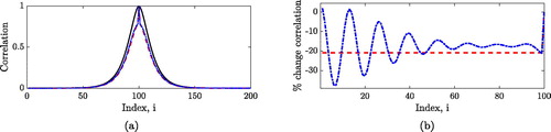
Figure 1a shows that for both methods, application of reconditioning reduces the value of off-diagonal correlations for all variables, with the largest absolute reduction occurring for variables closest to the observed variable. Although there is a large change to the off-diagonal correlations, we notice that the correlation lengthscale, which determines the rate of decay of the correlation function, is only reduced by a small amount. This shows that both methods of reconditioning dampen correlation values but do not significantly alter the overall pattern of correlation information. Figure 1b shows the percentage change to the original correlation values after reconditioning is applied. For RR, although the difference between the original correlation value and the reconditioned correlation depends on the index i, the relative change is constant across all off-diagonal correlations. As MVI does not alter the correlation matrix, it would correspond to a horizontal line through 0 for Fig. 1b.

When we directly plot the correlation values for the original and reconditioned matrices in Fig. 1a, the change to correlations for ME appears very similar to changes for RR. However, when we consider the percentage change to correlation in Fig. 1b, we see oscillation in the percentage differences of the ME correlations, showing that the relative effect on some spatially distant variables can be larger than for some spatially close variables. The spatial impact on individual variables differs significantly for this method. We also note that ME increases some correlation values. These are not visible in Fig. 1 due to entries in the original correlation matrix that are close to zero. Although the differences between $\mathbf{C}$ and ${\mathbf{C}}_{ME}$ far from the diagonal are small, small correlation values in the tails of the original SOAR matrix mean that when considering the percentage difference we obtain large values, as seen in Fig. 1b. This suggests that RR is a more appropriate method to use in this context, as the reconditioned matrix represents the initial correlation function better than ME, where spurious oscillations are introduced. These oscillations occur as ME changes the weighting of eigenvectors of the covariance matrix. As the eigenvectors of circulant matrices can be expressed in terms of discrete Fourier modes, ME has the effect of amplifying the eigenvalues corresponding to the highest frequency eigenvectors. This results in the introduction of spurious oscillations in correlation space.

Both methods reduce the correlation lengthscale of the error covariance matrix. In Tabeart et al. (2018), it was shown that reducing the lengthscale of the observation error covariance matrix decreases the condition number of the Hessian of the 3D-Var objective function and results in improved convergence of the minimisation problem. Hence, the application of reconditioning methods to the observation error covariance matrix is likely to improve convergence of the overall data assimilation problem. Fowler et al. (2018) studied the effect on the analysis of complex interactions between the background error correlation lengthscale, the observation error correlation lengthscale and the observation operator in idealised cases. Their findings for a fixed background error covariance, and direct observations, indicate that the effect of reducing the observation error correlation lengthscale (as in the reconditioned cases) is to increase the analysis sensitivity to the observations at larger scales. In other words, more weight is placed on the large-scale observation information content and less weight on the small scale observation information content. This corresponds with the findings of Section 3.5, where we proved that both methods of reconditioning reduce the weight on small scale observation information in the variational objective function. However, the lengthscale imposed by a more complex observation operator could modify these findings.

Example 2:

Interchannel correlations using an IASI covariance matrix

We now consider the impact of reconditioning on the IASI covariance matrix. We note that there is significant structure in the diagnosed correlations (see online resource 1), with blocks of highly correlated channels in the lower right-hand region of the matrix. We now consider how RR, ME and MVI change the variances and correlations of the IASI matrix.

Figure 2 shows the standard deviations $\mathbf{\Sigma },{\mathbf{\Sigma }}_{RR}$ and ${\mathbf{\Sigma }}_{ME}.$ These are calculated from the reconditioned matrices, but the values coincide with the theoretical results of Theorems 3 and 4. Standard deviation values for the original diagnosed case have been shown to be close to estimated noise characteristics of the instrument for each of the different channels (Stewart et al., 2014). We note that the largest increase to standard deviations occurs for channel 106 only and corresponds to a multiplicative inflation factor for this channel of 2.02 for RR and 1.81 for ME. Channel 106 is sensitive to water vapour and is the channel in the original diagnosed covariance matrix with the smallest standard deviation. The choice of ${\kappa }_{\mathit{max}}=100$ is of a similar size to the value of the parameters used at NWP centres (Weston, 2011; Weston et al., 2014; Bormann et al., 2016). This means that in practice, the contribution of observation information from channels where instrument noise is low is being substantially reduced.

Fig. 2. Standard deviations for the IASI covariance matrix $\mathbf{\Sigma }$ (black solid), ${\mathbf{\Sigma }}_{RR}$ (red dashed), ${\mathbf{\Sigma }}_{ME}$ (blue dot-dashed) for ${\kappa }_{\mathit{max}}=100.$

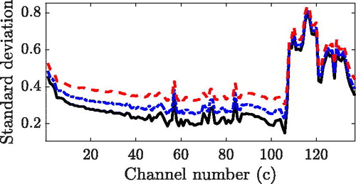
Channels are ordered by increasing wavenumber, and are grouped by type. We expect different wavenumbers to have different physical properties, and therefore different covariance structures. In particular, larger standard deviations are expected for higher wavenumbers due to additional sources of error (Weston et al., 2014), which is observed on the right-hand side of Fig. 2. For RR, larger increases to standard deviations are seen for channels with smaller standard deviations for the original diagnosed matrix than those with large standard deviations. This also occurs to some extent for ME, although we observe that the update term in (15)(15) $${\mathbf{\Sigma }}_{ME}(i,i)={\left(\mathbf{R}(i,i)+\sum _{k=1}^d{\mathbf{V}}_R{(i,k)}^2\mathbf{\Gamma }(k,k)\right)}^{1/2}.$$(15) is not constant in this case. This means that the reduction in weight in the analysis will not be uniform across different channels for ME. The result of Corollary 2 is satisfied; the increase to the variances is larger for RR than ME. This is particularly evident for channels where the variance from the original diagnosed covariance matrix is small. As MVI increases standard deviations by a constant factor, the largest changes for this method would occur for channels with large standard deviations in the original diagnosed matrix. This is in contrast to RR, where the largest changes occur for the channels in the original diagnosed matrix with the smallest standard deviation.

Figure 3 shows the difference between the diagnosed correlation matrix, $\mathbf{C},$ and the reconditioned correlation matrices ${\mathbf{C}}_{RR}$ and ${\mathbf{C}}_{ME}.$ As some correlations in the original IASI matrix are negative, we plot the entries of $(\mathbf{C}-{\mathbf{C}}_{RR})°\mathit{sign}(\mathbf{C})$ and $(\mathbf{C}-{\mathbf{C}}_{ME})°\mathit{sign}(\mathbf{C})$ in Fig. 3(a,b) respectively. Here $°$ denotes the Hadamard product, which multiplies matrices of the same dimension elementwise. This allows us to determine whether the magnitude of the correlation value is reduced by the reconditioning method; a positive value indicates that the reconditioning method reduces the magnitude of the correlation, whereas a negative value indicates an increase in the correlation magnitude. For RR, all differences are positive, which agrees with the result of Theorem 3. As MVI does not change the correlation matrix, an equivalent figure for this method is not given. We also note that there is a recognisable pattern in Fig. 3a, with the largest reductions occurring for the channels in the original diagnosed correlation matrix which were highly correlated. This indicates that this method of reconditioning does not affect all channels equally.

Fig. 3. Difference in correlations for IASI (a) $(\mathbf{C}-{\mathbf{C}}_{RR})°\mathit{sign}(\mathbf{C}),$ (b) $(\mathbf{C}-{\mathbf{C}}_{ME})°\mathit{sign}(\mathbf{C}),$ and (c) $({\mathbf{C}}_{ME}-{\mathbf{C}}_{RR})°\mathit{sign}(\mathbf{C}),$ where $°$ denotes the Hadamard product. Red indicates that the absolute correlation is decreased by reconditioning and blue indicates the absolute correlation is increased. The colourscale is the same for (a) and (b) but different for (c). Condition numbers of the corresponding covariance matrices are given by $\kappa (\mathbf{R})=2005.98,\kappa ({\mathbf{R}}_{RR})=100$ and $\kappa ({\mathbf{R}}_{ME})=100.$

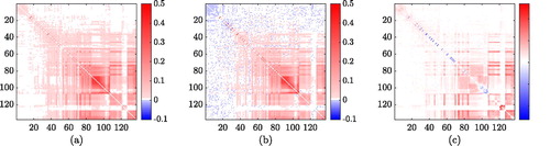
For ME, we notice that there are a number of entries where the absolute correlations are increased after reconditioning. There appears to be some pattern to these entries, with a large number occurring in the upper left-hand block of the matrix for channels with the smallest wavenumber (Weston et al., 2014). However, away from the diagonal for channels 0–40, where changes by RR are very small, the many entries where absolute correlations are increased by ME are much more scattered. This more noisy change to the correlations could be due to the fact that 96 eigenvalues are set to be equal to a threshold value by the minimum eigenvalue method in order to attain ${\kappa }_{\mathit{max}}=100.$ One method to reduce noise was suggested in Smith et al. (2018), which showed that applying localization methods (typically used to reduce spurious long-distance correlations that arise when using ensemble covariance matrices via the Schur product) after the reconditioning step can act to remove noise while retaining covariance structure.

For positive entries, the structure of ${\mathbf{C}}_{ME}$ appears similar to that of RR. There are some exceptions, however, such as the block of channels 121–126 where changes in correlation due to ME are small, but correlations are changed by quite a large amount for RR. The largest elementwise difference between RR and the original diagnosed correlation matrix is 0.138, whereas the largest elementwise difference between ME and the original diagnosed correlation matrix is 0.0036. The differences between correlations for ME and RR are shown in Fig. 3c.

For both methods, although the absolute value of all correlations is reduced, correlations for channels 1–70 are eliminated. This has the effect of emphasising the correlations for channels that are sensitive to water vapour. Weston et al. (2014) and Bormann et al. (2016) argue that much of the benefit of introducing correlated observation error for this instrument can be related to the inclusion of correlated error information for water vapour sensitive channels. Therefore, although the changes to the original diagnosed correlation matrix are large it is likely that a lot of the benefit of using correlated observation error matrices is retained.

We also note that it is more difficult to choose the best reconditioning method in this setting, due to the complex structure of the original diagnosed correlation matrix. In particular, improved understanding of how each method alters correlations and standard deviations is not enough to determine which method will perform best in an assimilation system. One motivation of reconditioning is to improve convergence of variational data assimilation algorithms. Therefore, one aspect of the system that can be used to select the most appropriate method of reconditioning is the speed of convergence. As ME results in repeated eigenvalues, we would expect faster convergence of conjugate gradient methods applied to the problem $\mathbf{Rx}=\mathbf{b}$ for $\mathbf{x},\mathbf{b}\in {\mathbb{R}}^d$ for ME than RR. However, Campbell et al. (2017), Weston (2011), Weston et al. (2014) and Bormann et al. (2015) find that RR results in faster convergence than ME for operational variational implementations. This is likely due to interaction between the reconditioned observation error covariance matrix and the observation operator, as the eigenvalues of ${\mathbf{H}}^T{\mathbf{R}}^{-1}\mathbf{H}$ are shown to be important for the conditioning of the variational data assimilation problem in Tabeart et al. (2018).

Another aspect of interest is the influence of reconditioning on the analysis and forecast performance. We note that this is likely to be highly system and metric-dependent. For example, Campbell et al. (2017) studied the impact of reconditioning on predictions of meteorological variables (temperature, geopotential height, precipitable water) over lead times from 0 to 5 days. In the U.S. Naval Research Laboratory system, ME performed slightly better at short lead times, whereas RR had improvements at longer lead times (Campbell et al., 2017). Differences in forecast performance were mixed, whereas convergence was much faster for RR. This meant that the preferred choice was RR. However, in the ECMWF system, Bormann et al. (2015) studied the standard deviation of first-guess departures against independent observations. Using this metric of analysis skill, ME was found to out-perform RR. The effect of RR on the analysis of the Met Office 1D-Var system is studied in Tabeart et al. (2019), where changes to retrieved variables sensitive to water vapour (humidity, variables sensitive to cloud) are found to be larger than for other meteorological variables such as temperature.

4.2.2. Changes to the analysis of a data assimilation problem

In Section 3.5, we considered how the variational objective function is altered by RR, ME and MVI. We found that the two methods of reconditioning reduced the weight on scales corresponding to small eigenvalues by a larger amount than MVI, which changes the weight on all scales uniformly. In this section, we consider how the analysis of an idealised data assimilation problem is altered by each of the three methods. We also consider how changing κ_max alters the analysis of the problem.

In order to compare the three methods, we study how the solution $\mathbf{x}$ of a conjugate gradient method applied to the linear system $\mathbf{Sx}=\mathbf{b}$ changes for RR, ME and MVI, where $\mathbf{S}={\mathbf{B}}^{-1}+{\mathbf{H}}^T{\mathbf{R}}^{-1}\mathbf{H}$ is the linearised Hessian associated with the 3D-Var objective function (24)(24) $$J(\mathbf{x})=\frac{1}{2}{(\mathbf{x}-{\mathbf{x}}_b)}^T{\mathbf{B}}^{-1}(\mathbf{x}-{\mathbf{x}}_b)+\frac{1}{2}{(\mathbf{y}-h[\mathbf{x}])}^T{\mathbf{R}}^{-1}(\mathbf{y}-h[\mathbf{x}]):=J_b+J_o$$(24) . To do this we define a ‘true’ solution, ${\mathbf{x}}_{\mathit{true}},$ construct the corresponding data $\mathbf{b}$ and assess how well we are able to recover ${\mathbf{x}}_{\mathit{true}}$ when applying RR, ME and MVI to $\mathbf{S}.$ Haben (2011) showed that this is equivalent to solving the 3D-Var objective function in the case of a linear observation operator. We define a background error covariance matrix, $\mathbf{B}\in {\mathbb{R}}^{200\times 200},$ which is a SOAR correlation matrix on the unit circle with correlation lengthscale 0.2 and a constant variance of 1. Our observation operator is given by the identity, meaning that every state variable is observed directly.

We construct a ‘true’ observation error covariance ${\mathbf{R}}_{\mathit{true}},$ given by a 200-dimensional SOAR matrix on the unit circle with standard deviation 1 and lengthscale 0.7. We then sample the Gaussian distribution with zero mean and covariance given by ${\mathbf{R}}_{\mathit{true}}$ 250 times and use these samples to calculate an estimated sample covariance matrix via the MATLAB function cov. This estimated sample covariance matrix ${\mathbf{R}}_{\mathit{est}}$ has condition number $\kappa ({\mathbf{R}}_{\mathit{est}})=3.95\times {10}^8.$ The largest estimated standard deviation is 1.07 and the smallest is 0.90, compared to the true constant standard deviation of 1. RR, ME and MVI are then applied to ${\mathbf{R}}_{\mathit{est}}$ with ${\kappa }_{\mathit{max}}=100.$ When applying MVI, we use two choices of α which correspond to changes to the standard deviations ${({\mathbf{R}}_{RR}(1,1))}^{1/2},{\alpha }_{RR}=1.41,$ and ${({\mathbf{R}}_{ME}(1,1))}^{1/2},{\alpha }_{ME}=1.39.$ The modified error covariance matrices will be denoted ${\mathbf{R}}_{\mathit{inflRR}}={\alpha }_{RR}^2{\mathbf{R}}_{\mathit{est}}$ and ${\mathbf{R}}_{\mathit{inflME}}={\alpha }_{ME}^2{\mathbf{R}}_{\mathit{est}}.$

We define a true state vector, (40) $$\mathbf{x}(k)=4\hspace{0.17em}\text{sin}\hspace{0.17em}(k\pi /100)-5.1\hspace{0.17em}\text{sin}\hspace{0.17em}(7k\pi /100)+1.5\hspace{0.17em}\text{sin}\hspace{0.17em}(12k\pi /100)-3\hspace{0.17em}\text{sin}\hspace{0.17em}(15k\pi /100)+0.75\hspace{0.17em}\text{sin}\hspace{0.17em}(45k\pi /100),$$(40) which has five scales. We then construct $\mathbf{b}\equiv \mathbf{Sx}$ using ${\mathbf{R}}_{\mathit{true}},$ and apply the MATLAB 2018b $\mathit{pcg}.m$ routine to the problem $({\mathbf{B}}^{-1}+{\mathbf{R}}^{-1})\mathbf{x}=\mathbf{b}$ for each choice of $\mathbf{R}.$ We recall that $\mathbf{S}={\mathbf{B}}^{-1}+{\mathbf{H}}^T{\mathbf{R}}^{-1}\mathbf{H}={\mathbf{B}}^{-1}+{\mathbf{R}}^{-1}$ as $\mathbf{H}=\mathbf{I}.$ Let ${\mathbf{x}}_{\mathit{est}}$ denote the solution that is found using ${\mathbf{R}}_{\mathit{est}}$ and ${\mathbf{x}}_{\mathit{mod}}$ refer to a solution found using a modified version of ${\mathbf{R}}_{\mathit{est}},$ namely ${\mathbf{R}}_{RR},{\mathbf{R}}_{ME},{\mathbf{R}}_{\mathit{inflRR}}$ or ${\mathbf{R}}_{\mathit{inflME}}.$ The maximum number of iterations allowed for the conjugate gradient routine is 200, and convergence is reached when the relative residual is less than $1\times {10}^{-6}.$

From Section 3.5, we expect RR, ME and MVI to behave differently at small and large scales. We therefore analyse how using each method alters the solution $\mathbf{x}$ at different scales using the discrete Fourier transform (DFT). This allows us to assess how well each scale of ${\mathbf{x}}_{\mathit{true}}$ is recovered for each choice of $\mathbf{R}.$ As ${\mathbf{x}}_{\mathit{true}}$ is the sum of sine functions, only the imaginary part of the DFT will be non-zero. We therefore define $a_{\mathit{true}}=\text{imag}(\mathit{DFT}(x_{\mathit{true}}));$ similarly $a_{\mathit{est}}=\text{imag}(\mathit{DFT}(x_{\mathit{est}}))$ and $a_{\mathit{mod}}=\text{imag}(\mathit{DFT}(x_{\mathit{mod}})).$

By construction, as $\mathbf{x},$ given by (40)(40) $$\mathbf{x}(k)=4\hspace{0.17em}\text{sin}\hspace{0.17em}(k\pi /100)-5.1\hspace{0.17em}\text{sin}\hspace{0.17em}(7k\pi /100)+1.5\hspace{0.17em}\text{sin}\hspace{0.17em}(12k\pi /100)-3\hspace{0.17em}\text{sin}\hspace{0.17em}(15k\pi /100)+0.75\hspace{0.17em}\text{sin}\hspace{0.17em}(45k\pi /100),$$(40) , is the sum of sine functions of period $2\pi n/200$ for $n=1,7,12,15,45,$ a_true returns a signal with 5 peaks, one for each value of n at frequency k = n. The amplitude for all other values of k is zero. For frequencies larger than 20, all choices of estimated and modified $\mathbf{R}$ recover a_true well. 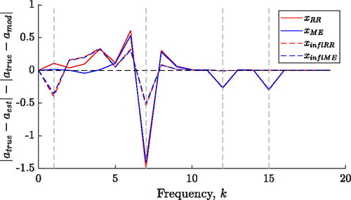Figure 4 shows the correction that is applied by the modified choices of $\mathbf{R}$ compared to ${\mathbf{R}}_{\mathit{est}}$ for the first 20 frequencies. A positive (negative) value shows that a_mod moves closer to (further from) a_true than a_est. The distance from 0 shows the size of this change. For the first true peak (k = 1) RR is able to move closer to a_true than a_est. However, both reconditioning methods move further from the truth at the location of true signals k = 7, 12, 15. For frequencies where a_est has a spurious non-zero signal RR and ME are able to move closer to a_true than a_est. At the location of true signals k = 7, 12, 15, MVI makes smaller changes compared to a_est than either method of reconditioning. 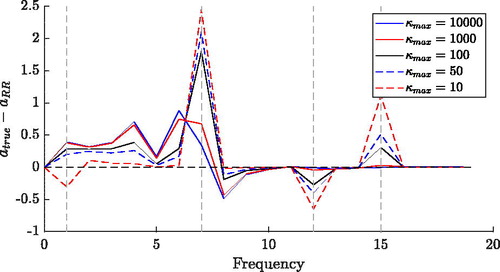As all modifications to ${\mathbf{R}}_{\mathit{est}}$ move a_mod further from a_true than a_est for k = 7, 12, 15, MVI is therefore better able to recover the value of a_true than RR or ME at these true peaks. However, MVI introduces a larger error for the first peak at k = 1 than RR or ME, and changes for frequencies k > 5 are much smaller than for reconditioning. This agrees with the findings of Section 3.5, that the weight on all scales is changed equally by MVI, whereas both methods of reconditioning result in larger changes to smaller scales and are hence able to make larger changes to amplitudes for higher frequencies. We recall from Section 3.5 that ME changes only the smaller scales, whereas RR also makes small changes to the larger scales. This behaviour is seen in Fig. 4: for frequencies k = 0 to 5 ME results in very small changes, with much larger changes for frequencies $5\le k\le 15.$ RR makes larger changes for larger values of k, but also moves closer to a_true for $1\le k\le 3.$

Fig. 4. Change in pointwise difference of discrete Fourier transform (DFT) from ${\mathbf{x}}_{\mathit{est}}$ to ${\mathbf{x}}_{\mathit{mod}}$ where a_est denotes the vector of coefficients of the imaginary part of $\mathit{DFT}({\mathbf{x}}_{\mathit{est}}).$ A positive (negative) value indicates that ${\mathbf{x}}_{\mathit{mod}}$ is closer to (further from) ${\mathbf{x}}_{\mathit{true}}$ than ${\mathbf{x}}_{\mathit{est}}$ and the amplitude shows how large this change is. Vertical dashed lines show the locations of non-zero values for the true signal.

We now consider how changing κ_max alters the quality of ${\mathbf{x}}_{RR}.$ As the behaviour for ${\kappa }_{\mathit{max}}=100$ shown in Fig. 4 was similar for both RR and ME, we only consider changes to RR. Figure 5 shows the difference between a_true and a_RR for different choices of κ_max. Firstly we consider the true signal that occurs at frequencies $k=1,7,12,15.$ For k = 1 the smallest error occurs for ${\kappa }_{\mathit{max}}=50$ and the largest error occurs for ${\kappa }_{\mathit{max}}=10000.$ For k = 7, 12, 15 the error increases as κ_max decreases. For all other frequencies, reducing κ_max reduces the error in the spurious non-zero amplitudes. For very large values of κ_max, we obtain small errors for the true signal, but larger spurious errors elsewhere. Very small values of κ_max can control these spurious errors, but fail to recover the correct amplitude for the true signal. Therefore a larger reconditioning constant will result in larger changes to the analysis. This means that there is a balance to be made in ensuring the true signal is captured, but spurious signal is depressed. For this framework a choice of ${\kappa }_{\mathit{max}}=100$ provides a good compromise between recovering the true peaks well and suppressing spurious correlations.

Fig. 5. Difference between a_true and a_RR for different choices of κ_max. Vertical dashed lines show the locations of non-zero values for the true signal.

Finally, Table 2 shows how convergence of the conjugate gradient method is altered by the use of reconditioning and MVI. Using a larger inflation constant for MVI does lead to slightly faster convergence compared to ${\mathbf{R}}_{\mathit{est}}.$ However, reducing κ_max leads to a much larger reduction in the number of iterations required for convergence for both RR and ME. This agrees with results in operational data assimilation systems, where the choice of κ_max and reconditioning method makes a difference to convergence (Weston, 2011; Tabeart et al., 2019).

Table 2 Changes to convergence of RR, MI and MVI for different values of κ_max.

κmax	10, 000	1, 000	100	50	10
RR	245	244	170	141	73
ME	240	239	193	145	76
Infl RR	244	244	238	233	199

For all choices of κ_max, convergence for ${\mathbf{R}}_{\mathit{true}}$ occurs in 17 iterations and ${\mathbf{R}}_{\mathit{est}}$ occurs in 244 iterations.

5. Conclusions

Applications of covariance matrices often arise in high dimensional problems (Pourahmadi, 2013), such as NWP (Weston et al., 2014; Bormann et al., 2016). In this paper we have examined two methods that are currently used at NWP centres to recondition covariance matrices by altering the spectrum of the original covariance matrix: the ridge regression method, where all eigenvalues are increased by a fixed value, and the minimum eigenvalue method, where eigenvalues smaller than a threshold are increased to equal the threshold value. We have also considered multiplicative variance inflation, which does not change the condition number or rank of a covariance matrix, but is used at NWP centres (Bormann et al., 2016).

For both reconditioning methods, we developed new theory describing how variances are altered. In particular, we showed that both methods will increase variances, and that this increase is larger for the ridge regression method. We also showed that applying the ridge regression method reduces all correlations between different variables. Comparing the impact of reconditioning methods and multiplicative variance inflation on the variational data assimilation objective function we find that all methods reduce the weight on observation information in the analysis. However, reconditioning methods have a larger effect on smaller eigenvalues, whereas multiplicative variance inflation does not change the sensitivity of the analysis to different scales. We then tested both methods of reconditioning and multiplicative variance inflation numerically on two examples: Example 1, a spatial covariance matrix, and Example 2, a covariance matrix arising from NWP. In Section 4.2, we illustrated the theory developed earlier in the work, and also demonstrated that for two contrasting numerical frameworks, the change to the correlations and variances is significantly smaller for the majority of entries for the minimum eigenvalue method.

Both reconditioning methods depend on the choice of κ_max, an optimal choice of which will depend on the specific problem in terms of computational resource and required precision. The smaller the choice of κ_max, the more variances and correlations are altered, so it is desirable to select the largest condition number that the system of interest can deal with. Some aspects of a system that could provide insight into reasonable choices of κ_max are:

• For conjugate gradient methods, the condition number provides an upper bound on the rate of convergence for the problem $A\mathbf{x}=\mathbf{b}$ (Golub and Van Loan, 1996), and can provide an indication of the number of iterations required to reach a particular precision (Axelsson, 1996). Hence, κ_max could be chosen such that a required level of precision is guaranteed for a given number of iterations.

• For more general methods, the condition number can provide an indication of the number of digits of accuracy that are lost during computations (Gill et al., 1986; Cheney, 2005). Knowledge of the error introduced by other system components, such as approximations in linearised observation operators and linearised models, relative resolution of the observation network and state variables, precision and calibration of observing instruments, may give insight into a value of κ_max that will maintain the level of precision of the overall problem.

• The condition number measures how errors in the data are amplified when inverting the matrix of interest (Golub and Van Loan, 1996). Again, the magnitude of errors resulting from other aspects of the system may give an indication of a value of κ_max that will not dominate the overall precision.

For our experiments, we considered choices of κ_max in the range $100-1000.$ For Experiment 2 these values are similar to those considered for the same instrument at different NWP centres e.g. 25, 100, 1000 (Weston, 2011), 67 (Weston et al., 2014), 54 and 493 (Bormann et al., 2015), 169 (Campbell et al., 2017). We note that the dimension of this interchannel error covariance matrix in operational practice is small and only forms a small block of the full observation error covariance matrix. Additionally, the matrix considered in this paper corresponds to one observation type; there are many other observation types with different error characteristics.

In this work, we have assumed that our estimated covariance matrices represent the desired correlation matrix well, in which case the above conditions on κ_max can be used. This is not true in general, and it may be that methods such as inflation and localisation are also required in order to constrain the sources of uncertainty that are underestimated or mis-specified. In this case, the guidance we have presented in this paper concerning how to select the most appropriate choice of reconditioning method and target condition number will need to be adapted. Additionally, localisation alters the condition number of a covariance matrix as a side effect; the user does not have the ability to choose the target condition number κ_max or control changes to the distribution of eigenvalues (Smith et al., 2018). This indicates that reconditioning may still be needed in order to retain valuable correlation information whilst ensuring that the computation of the inverse covariance matrix is feasible.

The choice of which method is most appropriate for a given situation depends on the system being used and the depth of user knowledge of the characteristics of the error statistics. The ridge regression method preserves eigenstructure by increasing the weight of all eigenvalues by the same amount, compared to the minimum eigenvalue method which only increases the weight of small eigenvalues and introduces a large number of repeated eigenvalues. We have found that ridge regression results in constant changes to variances and strict decreases to absolute correlation values, whereas the minimum eigenvalue method makes smaller, non-monotonic changes to correlations and non-constant changes to variances. In the spatial setting, the minimum eigenvalue method introduced spurious correlations, whereas ridge regression resulted in a constant percentage reduction for all variables. In the inter-channel case, changes to standard deviations and most correlations were smaller for the minimum eigenvalue method than for ridge regression.

Another important property for reconditioning methods is the speed of convergence of minimisation of variational data assimilation problems. It is well known that other aspects of matrix structure, such as repeated or clustered eigenvalues, are important for the speed of convergence of conjugate gradient minimisation problems. As the condition number is only sensitive to the extreme eigenvalues, conditioning alone cannot fully characterise the expected convergence behaviour. In the data assimilation setting, complex interactions occur between the constituent matrices (Tabeart et al., 2018), which can make it hard to determine the best reconditioning method a priori. One example of this is seen for operational implementations in Campbell et al. (2017) and Weston (2011) where the ridge regression method results in fewer iterations for a minimisation procedure than the minimum eigenvalue method, even though the minimum eigenvalue method yields observation error covariance matrices with a large number of repeated eigenvalues. Furthermore, Tabeart et al. (2018) found cases in an idealised numerical framework where increasing the condition number of the Hessian of the data assimilation problem was linked to faster convergence of the minimisation procedure. Again, this was due to interacting eigenstructures between observation and background terms, which could not be measured by the condition number alone. Additionally, Haben (2011) and Tabeart et al. (2018) find that the ratio of background to observation error variance is important for the convergence of a conjugate gradient problem. In the case where observation errors are small, poor performance of conjugate gradient methods is therefore likely. This shows that changes to the analysis of data assimilation problems due to the application of reconditioning methods are likely to be highly system-dependent, for example due to: quality of estimated covariance matrices, interaction between background and observation error covariance matrices, specific implementations of the assimilation algorithm, and choice of preconditioner and minimisation routine. However, the improved understanding of alterations to correlations and standard deviations for each method of reconditioning provided here may allow users to anticipate changes to the analysis for a particular system of interest using the results from previous idealised and operational studies (e.g. Weston et al., 2014; Bormann et al., 2016; Fowler et al., 2018; Tabeart et al., 2018; Simonin et al., 2019).

Acknowledgements

Thanks to Stefano Migliorini and Fiona Smith at the UK Met Office for the provision of the IASI matrix.

Disclosure statement

No potential conflict of interest was reported by the authors.

Additional information

Funding

This work is funded in part by the EPSRC Centre for Doctoral Training in Mathematics of Planet Earth, the NERC Flooding from Intense Rainfall Programme (NE/K008900/1), the EPSRC DARE project (EP/P002331/1) and the NERC National Centre for Earth Observation.

Appendix

Equivalence of the minimum eigenvalue method with the Ky-Fan 1-d norm method

We introduce the Ky-Fan p – k norm. We show that the solution to a nearest matrix problem to $\mathbf{X}\in {\mathrm{ℝ}}^{d\times d}$ in the Ky-Fan $1-d$ norm is equivalent to the minimum eigenvalue method of reconditioning introduced in Section 2.2 with an additional assumption.

Definition A.3.

The Ky-Fan p-k norm of $\mathbf{X}\in {\mathbb{C}}^{m\times n}$ is defined as: (A.1) $$\left|\right|\mathbf{X}|{|}_{p,k}={\left(\sum _{i=1}^k{\gamma }_i{(\mathbf{X})}^p\right)}^{1/p},$$(A.1) where ${\gamma }_i(\mathbf{X})$ denotes the i-th largest singular value of $\mathbf{X},$ $p\ge 1$ and $k\in \{1,\dots ,\min \{m,n\left\}\right\}.$

As covariance matrices are positive semi-definite by definition, the singular values of a covariance matrix $\mathbf{X}\in {\mathbb{R}}^{d\times d}$ are equal to its eigenvalues.

Theorem A.1.

Let $\mathbf{X}\in {\mathbb{R}}^{d\times d}$ be a symmetric positive semi-definite matrix, with eigenvalues ${\lambda }_1\ge {\lambda }_2\ge \dots \ge {\lambda }_d\ge 0$ and corresponding matrix of eigenvectors given by ${\mathbf{V}}_{\mathbf{R}}$. The choice of $\widehat{\mathbf{X}}$ that minimises (A.2) $$\left|\right|\mathbf{X}-\widehat{\mathbf{X}}|{|}_{1,p},$$(A.2) subject to the condition $\kappa (\widehat{\mathbf{X}})=\widehat{\kappa },$ for $\widehat{\kappa }\ge d-l+1$, is given by $\widehat{\mathbf{X}}={\mathbf{V}}_{\mathbf{R}}D\mathit{iag}({\lambda }^{*}){\mathbf{V}}_{\mathbf{R}}^T,$ where ${\lambda }^{*}$ is defined by (A.3) $${\lambda }_k^{*}=\{\begin{array}{c}{\mu }^{*}:=\frac{{\lambda }_1}{\widehat{\kappa }}if{\lambda }_k<{\mu }^{*}\hfill \\ {\lambda }_k^{*}={\lambda }_k\mathit{otherwise}\hfill \end{array}$$(A.3) and where l is the index such that ${\lambda }_l\le {\mu }^{*}<{\lambda }_{l-1}.$

Proof.

We apply the result given in Theorem 4 of Tanaka and Nakata (2014) for the trace norm (defined as p = 1 and k = d) to find the optimal value of ${\mu }^{*}.$ Theorem 2 of the same work yields the minimising solution $\widehat{\mathbf{X}}$ for the value of ${\mu }^{*}.$

We remark that the statement of Theorem 4 of Tanaka and Nakata (2014) uses the stronger assumption that $\widehat{\kappa }\ge d.$ However, a careful reading of the proof of this theorem indicates that a weaker assumption is sufficient: we assume that $\widehat{\kappa }>d-l+1$ where l is the index such that ${\lambda }_l\le {\mu }^{*}<{\lambda }_{l-1}.$ □

We note that this optimal value of ${\mu }^{*}$ is the same as the threshold $T=\frac{{\lambda }_1}{\widehat{\kappa }}$ defined for the minimum eigenvalue method in (5(5) $${\lambda }_k({\mathbf{R}}_{ME})=\{\begin{array}{cc}{\lambda }_k(\mathbf{R})\hfill & \text{if}{\lambda }_k(\mathbf{R})>T\hfill \\ T\hfill & \text{if}{\lambda }_k(\mathbf{R})\le T\hfill \end{array}.$$(5) ) and hence the minimum eigenvalue method is equivalent to the Ky-Fan 1-d minimizer of (A.2)(A.2) $$\left|\right|\mathbf{X}-\widehat{\mathbf{X}}|{|}_{1,p},$$(A.2) in the case that $\kappa \ge d-l+1.$

The minimum eigenvalue method is still a valid method of reconditioning when the additional assumption on the eigenvalues of $\mathbf{X}$ is not satisfied. In particular, in the experiments considered in Section 4 we see qualitatively similar behaviour for the choices of T that satisfy the assumption, and those that do not. It is possible that the lower bound on the condition number imposed by the additional constraint on κ_max could provide guidance on the selection of the target condition number.

References

- Axelsson, O. 1996. Iterative Solution Methods. Cambridge: Cambridge University Press.
- Bannister, R. N. 2017. A review of operational methods of variational and ensemble variational data assimilation. Q. J. R. Meteorol. Soc. 143, 607–633. doi:10.1002/qj.2982
- Bickel, P. J. and Levina, E. 2008. Covariance regularization by thresholding. Ann. Stat. 36, 2577–2604. doi:10.1214/08-AOS600
- Bormann, N., Bonavita, M., Dragani, R., Eresmaa, R., Matricardi, M. and co-authors. 2015. Enhancing the Impact of IASI Observations through an Updated Observation Error Covariance Matrix. ECMWF Technical Memoranda. ECMWF, Reading.
- Bormann, N., Bonavita, M., Dragani, R., Eresmaa, R., Matricardi, M. and co-authors. 2016. Enhancing the impact of IASI observations through an updated observation error covariance matrix. Q. J. R. Meteorol. Soc. 142, 1767–1780. doi:10.1002/qj.2774
- Budd, C. J., Freitag, M. A. and Nichols, N. K. 2011. Regularization techniques for ill-posed inverse problems in data assimilation. Comput. Fluids 46, 168–173. doi:10.1016/j.compfluid.2010.10.002
- Campbell, W. F., Satterfield, E. A., Ruston, B. and Baker, N. L. 2017. Accounting for correlated observation error in a dual-formulation 4D variational data assimilation system. Mon. Wea. Rev. 145, 1019–1032. doi:10.1175/MWR-D-16-0240.1
- Cheney, W. 2005. Numerical Mathematics and Computing. 5th ed., International ed. Brooks/Cole Cengage Learning, Pacific Grove, CA.
- Cordoba, M., Dance, S. L., Kelly, G. A., Nichols, N. K. and Waller, J. A. 2016. Diagnosing atmospheric motion vector observation errors for an operational high resolution data assimilation system. Q. J. R. Meteorol. Soc. 143, 333–341.
- Daley, R. 1991. Atmospheric Data Analysis. Cambridge University Press, New York.
- Desroziers, G., Berre, L., Chapnik, B. and Poli, P. 2005. Diagnosis of observation, background and analysis-error statistics in observation space. Q. J. R. Meteorol. Soc. 131, 3385–3396. doi:10.1256/qj.05.108
- Fan, K. 1959. Convex sets and their applications. Lecture notes. Applied Mathematics Division, Argonne National Laboratory, Lemont, IL.
- Fowler, A. M., Dance, S. L. and Waller, J. A. 2018. On the interaction of observation and prior error correlations in data assimilation. Q. J. R. Meteorol. Soc. 144, 48–62. doi:10.1002/qj.3183
- Ghil, M. 1989. Meteorological data assimilation for oceanographers. Part I: description and theoretical framework. Dyn. Atmos. Oceans. 13, 171–218. doi:10.1016/0377-0265(89)90040-7
- Ghil, M. and Malanotte-Rizzoli, P. 1991. Data assimilation in meteorology and oceanography. Adv. Geophys. 33, 141–266. doi:10.1016/S0065-2687(08)60442-2
- Gill, P. E., Murray, W. and Wright, M. H. 1986. Practical Optimization. Academic Press, Amsterdam/London.
- Golub, G. H. and Van Loan, C. F. 1996. Matrix Computations. 3rd ed. The John Hopkins University Press, Baltimore, MD.
- Gray, R. M. 2006. Toeplitz and circulant matrices: a review. Found. Trends Commun. Inform. Theory 2, 155–239.
- Guillet, O., Weaver, A. T., Vasseur, X., Michel, Y., Gratton, S. and co-authors. 2019. Modelling spatially correlated observation errors in variational data assimilation using a diffusion operator on an unstructured mesh. Q. J. R. Meteorol. Soc. 145, 1947–1967. doi:10.1002/qj.3537
- Haben, S. A. 2011. Conditioning and preconditioning of the minimisation problem in variational data assimilation. PhD thesis, Department of Mathematics and Statistics, University of Reading, Reading.
- Haben, S. A., Lawless, A. S. and Nichols, N. K. 2011a. Conditioning and preconditioning of the variational data assimilation problem. Comput. Fluids 46, 252–256. doi:10.1016/j.compfluid.2010.11.025
- Haben, S. A., Lawless, A. S. and Nichols, N. K. 2011b. Conditioning of incremental variational data assimilation, with application to the Met Office system. Tellus A 64, 782–792.
- Hamill, T. M., Whitaker, J. S. and Snyder, C. 2001. Distance-dependent filtering of background error covariance estimates in an ensemble Kalman filter. Mon. Wea. Rev. 129, 2776–2790. doi:10.1175/1520-0493(2001)129<2776:DDFOBE>2.0.CO;2
- Hansen, P. C. 1998. Rank-Deficient and Discrete Ill-Posed Problems: Numerical Aspects of Linear Inversion. Society for Industrial and Applied Mathematics, Philadelphia, PA.
- Healy, S. B. and White, A. A. 2005. Use of discrete Fourier transforms in the 1D-Var retrieval problem. Q. J. R. Meteorol. Soc. 131, 63–72. doi:10.1256/qj.03.193
- Heilliette, S. and Garand, L. 2015. Impact of accounting for inter-channel error covariances at the Canadian meteorological centre. In: Proceedings of the 2015 EUMETSAT Meteorological Satellite Conference, Toulouse, France, p. 8. Online at: https://www.eumetsat.int/website/home/News/ConferencesandEvents/PreviousEvents/DAT_2305526.html
- Higham, N. J. 2002. Computing the nearest correlation matrix – a problem from finance. IMA J. Numer. Anal. 22, 329–343. doi:10.1093/imanum/22.3.329
- Higham, N. J., Strabić, N. and Šego, V. 2016. Restoring definiteness via shrinking, with an application to correlation matrices with a fixed block. SIAM Rev. 58, 245–263. doi:10.1137/140996112
- Hoerl, A. E. and Kennard, R. W. 1970. Ridge regression: biased estimation for nonorthogonal problems. Technometrics 12, 55–67. doi:10.1080/00401706.1970.10488634
- Horn, R. A. and Johnson, C. R. 1991. Topics in Matrix Analysis. Cambridge University Press, Cambridge.
- Janjić, T., Bormann, N., Bocquet, M., Carton, J. A., Cohn, S. E. and co-authors. 2018. On the representation error in data assimilation. Q. J. R. Meteorol. Soc. 144, 1257–1278. doi:10.1002/qj.3130
- Johnson, C., Hoskins, B. J. and Nichols, N. K. 2005. A singular vector perspective of 4D-Var: filtering and interpolation. Q. J. R. Meteorol. Soc. 131, 1–19. doi:10.1256/qj.03.231
- Ledoit, O. and Wolf, M. 2004. A well-conditioned estimator for large-dimensional covariance matrix. J. Multivar. Anal. 88, 365–411. doi:10.1016/S0047-259X(03)00096-4
- Liu, Z.-Q. and Rabier, F. 2003. The potential of high-density observations for numerical weather prediction: a study with simulated observations. Q. J. R. Meteorol. Soc. 129, 3013–3035. doi:10.1256/qj.02.170
- McNally, A. P., Watts, P. D., Smith, J. A., Engelen, R., Kelly, G. A. and co-authors. 2006. The assimilation of AIRS radiance data at ECMWF. Q. J. R. Meteorol. Soc. 132, 935–957. doi:10.1256/qj.04.171
- Ménétrier, B., Montmerle, T., Michel, Y. and Berre, L. 2015. Linear filtering of sample covariances for ensemble-based data assimilation. Part I: optimality criteria and application to variance filtering and covariance localization. Mon. Wea. Rev. 143, 1622–1643. doi:10.1175/MWR-D-14-00157.1
- Michel, Y. 2018. Revisiting Fisher’s approach to the handling of horizontal spatial correlations of the observation errors in a variational framework. Q. J. R. Meteorol. Soc. 144, 2011–2025. doi:10.1002/qj.3249
- Migliorini, S. 2012. On the equivalence between radiance and retrieval assimilation. Mon. Wea. Rev. 140, 258–265. doi:10.1175/MWR-D-10-05047.1
- Moodey, A. J. F., Lawless, A. S., Potthast, R. W. E. and van Leeuwen, P. J. 2013. Nonlinear error dynamics for cycled data assimilation methods. Inverse Probl. 29, 025002. doi:10.1088/0266-5611/29/2/025002
- Nakamura, G. and Potthast, R. 2015. Inverse Modeling. Bristol: IOP Publishing, pp. 2053–2563.
- Pourahmadi, M. 2013. High-Dimensional Covariance Estimation. John Wiley & Sons, Hoboken, NJ.
- Prates, C., Migliorini, S., Stewart, L. and Eyre, J. 2016. Assimilation of transformed retrievals obtained from clear-sky IASI measurements. Q. J. R. Meteorol. Soc. 142, 1697–1712. doi:10.1002/qj.2764
- Qi, H. and Sun, D. 2010. Correlation stress testing for value-at-risk: an unconstrained convex optimization approach. Comput. Optim. Appl. 45, 427–462. doi:10.1007/s10589-008-9231-4
- Schiff, S. J. 2011. Neural Control Engineering: The Emerging Intersection between Control Theory and Neuroscience. Computational Neuroscience. MIT Press, Cambridge, MA.
- Simonin, D., Waller, J. A., Ballard, S. P., Dance, S. L. and Nichols, N. K. 2019. A pragmatic strategy for implementing spatially correlated observation errors in an operational system: demonstration for Doppler radar winds. Q. J. R. Meteorol. Soc. 145, 2772–2790. doi:10.1002/qj.3592
- Skøien, J. O. and Blöschl, G. 2006. Sampling scale effects in random fields and implications for environmental monitoring. Environ. Monit. Assess. 114, 521–552. doi:10.1007/s10661-006-4939-z
- Smith, P. J., Lawless, A. S. and Nichols, N. K. 2018. Treating sample covariances for use in strongly coupled atmosphere-ocean data assimilation. Geophys. Res. Lett. 45, 445–454. doi:10.1002/2017GL075534
- Stewart, L. M. 2010. Correlated observation errors in data assimilation. PhD thesis, University of Reading, Reading.
- Stewart, L. M., Cameron, J., Dance, S. L., English, S., Eyre, J. and Nichols, N. K. 2009. Observation Error Correlations in IASI Radiance Data. Mathematics Report Series, Report number 1/2009, University of Reading, Reading.
- Stewart, L. M., Dance, S. L. and Nichols, N. K. 2008. Correlated observation errors in data assimilation. Int. J. Numer. Meth. Fluids 56, 1521–1527. doi:10.1002/fld.1636
- Stewart, L. M., Dance, S. L. and Nichols, N. K. 2013. Data assimilation with correlated observation errors: experiments with a 1-D shallow water model. Tellus A 65, 19546 (14 pp.), doi:10.3402/tellusa.v65i0.19546
- Stewart, L. M., Dance, S. L., Nichols, N. K., Eyre, J. R. and Cameron, J. 2014. Estimating interchannel observation-error correlations of IASI radiance data in the Met Office system. Q. J. R. Meteorol. Soc. 140, 1236–1244. doi:10.1002/qj.2211
- Tabeart, J. M., Dance, S. L., Haben, S. A., Lawless, A. S., Nichols, N. K. and Waller, J. A. 2018. The conditioning of least squares problems in variational data assimilation. Numer. Linear Algebra Appl. 25, e2165. doi:10.1002/nla.2165
- Tabeart, J. M., Dance, S. L., Lawless, A. S., Migliorini, S., Nichols, N. K., and co-authors.2019. The impact of reconditioning of the correlated observation error covariance matrix on the Met Office system. Online at: http://arxiv.org/abs/1908.04071. Submitted.
- Tanaka, M. and Nakata, K. 2014. Positive definite matrix approximation with condition number constraint. Optim. Lett. 8, 939–947. doi:10.1007/s11590-013-0632-7
- Thiebaux, H. J. 1976. Anisotropic correlation functions for objective analysis. Mon. Wea. Rev. 104, 994–1002. doi:10.1175/1520-0493(1976)104<0994:ACFFOA>2.0.CO;2
- Trefethen, L. N. and Bau, D. 1997. Numerical Linear Algebra. Society for Industrial and Applied Mathematics, Philadelphia, PA.
- Waller, J. A., Ballard, S. P., Dance, S. L., Kelly, G., Nichols, N. K. and Simonin, D. 2016. Diagnosing horizontal and inter-channel observation error correlations for SEVIRI observations using observation-minus-background and observation-minus-analysis statistics. Remote Sens. 8, 581. doi:10.3390/rs8070581
- Waller, J. A., Dance, S. L. and Nichols, N. K. 2016. Theoretical insight into diagnosing observation error correlations using observation-minus-background and observation-minus-analysis statistics. Q. J. R. Meteorol. Soc. 142, 418–431. doi:10.1002/qj.2661
- Waller, J. A., Simonin, D., Dance, S. L., Nichols, N. K. and Ballard, S. P. 2016. Diagnosing observation error correlations for Doppler radar radial winds in the Met Office UKV model using observation-minus-background and observation-minus-analysis statistics. Mon. Wea. Rev. 144, 3533–3551. doi:10.1175/MWR-D-15-0340.1
- Weston, P. 2011. Progress towards the Implementation of Correlated Observation Errors in 4D-Var. Forecasting Research Technical Report 560, Met Office, Exeter, UK.
- Weston, P. P., Bell, W. and Eyre, J. R. 2014. Accounting for correlated error in the assimilation of high-resolution sounder data. Q. J. R. Meteorol. Soc. 140, 2420–2429. doi:10.1002/qj.2306
- Yaglom, A. M. 1987. Correlation Theory of Stationary and Related Random Functions, Volume I: Basic Results. Springer-Verlag, New York.