A balanced state consistent with planetary-scale motion for quasi-geostrophic dynamics

Abstract

The role of planetary-scale zonally-asymmetric thermal forcing on large-scale atmospheric dynamics is crucial for understanding low-frequency phenomena in the atmosphere. Despite its paramount importance, good theoretical foundation for the understanding is still lacking. Here, we address this issue by providing a general framework for including planetary-scale thermal forcing in large-scale atmospheric dynamics studies. This is accomplished by identifying two distinct geostrophic motions of horizontal length scale L in terms of the external Rossby deformation length scale L_D: i) $L\sim {ϵ}^0{L}_D$ and ii) $L\sim {ϵ}^{1/2}{L}_D,$ where ϵ is the Rossby number. In addition, via multi-scale analysis, we show that the large-scale atmospheric dynamics can be described by mutual interaction between the two scales. The analysis results in planetary geostrophic equations with large-scale thermal forcing that provide the basic balanced states for processes such as the growth of synoptic waves. In the long-time limit, the continuous growth and decay of synoptic waves provide the convergence of horizontal heat and vorticity fluxes, which contributes to the energy flux balance in the planetary geostrophic scale with planetary-scale advection and thermal forcing.

Keywords:

• planetary geostrophic motion
• quasi-geostrophic motion
• multi-scale analysis

1. Introduction

The effects of zonally-varying thermodynamic or orographic forcing on large-scale atmospheric motions have been a main topic of investigation in atmospheric dynamics studies. This is because of the forcing’s possible relationship to storm tracks (Chang et al., 2002), large-scale atmospheric stationary waves (Held, 1983) and low-frequency variability, such as the North Atlantic Oscillation (Marshall et al., 2001) and Pacific North Atlantic mode (Leathers et al., 1991). However, despite this importance, adequate theoretical understanding is still lacking. In general, zonally-symmetric state is still widely used in fundamental numerical studies with idealized forcing (see, e.g. Polvani et al., 2004).

Zonally-asymmetric forcing poses a major challenge in dynamics studies. This is because obtaining a state in balance with an asymmetric thermal forcing is not trivial. For example, a radiative-convective equilibrium state with thermal wind balance does not automatically determine a basic balanced state for zonally-varying thermal forcing – as in the zonally-symmetric case. A possibility still exists for finding a statistically-stationary state with a zonally-asymmetric forcing. However, the connection between initial balanced state and subsequent growth of transient eddies is then lost.

Traditionally, zonally-symmetric states have been used to understand large-scale, quasi-geostrophic (QG) dynamics at the mid-latitude. In particular, linearized QG equations have mainly been used for baroclinic instability, addressing the linear growth rate of large-scale atmospheric waves and associated poleward heat transfer (e.g. Charney, 1947; Eady, 1949; Phillips, 1954). The full QG equation is an approximation of the primitive equations with a specific temporal and spatial scale associated with large-scale atmospheric dynamics (Pedlosky, 2013). Choosing the main spatial scale L to be the internal Rossby deformation radius ($\approx$1000 km), the leading-order equations based on small Rossby number, $ϵ\equiv U/(fL)$ with U the characteristic speed for the structure of length scale L, are as follows: (1a) $$\frac{1}{\rho }\frac{\partial P}{\partial x}=fv$$(1a) (1b) $$\frac{1}{\rho }\frac{\partial P}{\partial y}=-fu$$(1b) (1c) $$\frac{\partial P}{\partial z}=-\rho g,$$(1c) where P is the pressure; f is the Coriolis parameter for the mid-latitude; u and v are the zonal and meridional velocities, respectively; and ρ is the density. Given that there are three equations and four (leading order) variables, the variables are not determined uniquely at this order: the next order is required to close the system.

Broadly, the large-scale, synoptic motion is driven by the temperature contrast between low and high latitudes, due to the latitudinal imbalance of radiative-convective thermal forcing. Hence, an often-used balanced initial condition in numerical simulations is one obtained by combining thermal wind balance and meridional radiative-convective equilibrium temperature distribution: (2) $$f\frac{\partial U^{*}}{\partial \hspace{0.17em}\text{log}\hspace{0.17em}P}=\frac{R}{a}\frac{\partial T}{\partial \theta },$$(2) where $U^{*}(\theta ,P)$ is the balanced zonal wind with θ the latitude; $T_E(\theta ,P)$ is the radiative-convective balanced temperature; R is the gas constant for air; and a is the Earth’s radius (Simmons and Hoskins, 1977, 1978). However, this raises a fundamental consistency issue: the leading-order variables in the QG equations are determined only at the next order, $O(ϵ$), but the balanced zonal wind is obtained without recourse to the higher order. Here note that T_E is the solution of the primitive equations (specifically, the heat equation) at leading order, rather than of Eq. (1)(1a) $$\frac{1}{\rho }\frac{\partial P}{\partial x}=fv$$(1a) . When considering a zonally-asymmetric situation such as that arising from land–sea contrast, for example, thermal wind balance cannot be used to construct a balanced state which addresses that asymmetry.

The contribution of eddies to the shaping of large-scale atmospheric circulation is well understood in the zonally-symmetric case (see, e.g. Schneider, 2006), but poorly understood in the zonally-asymmetric case. One reason for this is because the wave-mean flow interaction, a useful diagnostic concept in the zonally-symmetric case, becomes ambiguous in the asymmetric case since zonal-mean state can no longer be used as the mean. It is possible to use the concept of stationary waves to represent the effect of zonally-asymmetric thermodynamic or orographic forcing on the zonal mean (Held, 1983). Here, the zonal symmetry can be represented at the leading order and the asymmetry can be treated as stationary waves on the symmetric behaviour at the next order. However, while this distinction is useful for analysing the effect of the zonally-asymmetric forcing, the interaction between stationary waves and transient eddies is not described in this decomposition.

Consider now the planetary scale, where $L\sim a,$ where a is the radius of Earth. The notion of planetary geostrophic (PG) motion has been introduced by Welander (1959) to explain the global thermocline structure of the ocean. Interestingly, the leading order PG equations are closed – i.e. it is not necessary to consider the next order to determine the leading order variables. In particular, the heat equation included in the leading order can take a global-scale thermodynamic forcing. Following this, PG motion for the large-scale atmosphere has been introduced by Phillips (1963), wherein it is named ‘geostrophic motion of type 2’. Significantly, in that study it is noted that large-scale flows would need to be forced to maintain the balance in the type 2 geostrophic motion. This suggests that the PG motion could serve in constructing a more physically realistic balanced state consistent with a zonally-asymmetric forcing. Indeed, in this paper we elucidate the relationship between PG and QG motions and address how to deal with QG dynamics in the presence of planetary-scale zonally-asymmetric forcing.

Recently, careful studies of the relationship between planetary and synoptic scales in PG motions have been undertaken by Dolaptchiev and Klein (2009, 2013) using multi-scale analysis. In their studies, perturbation analysis is based on the small parameter, ${(a{\Omega }^2/g)}^{1/3},$ where Ω is the angular speed of Earth’s rotation. Other parameters in the problem – such as the Mach, Froude, and Rossby numbers – are expressed in terms of this small parameter, showing the relationships among different scales via the analysis. The overall results for the mutual relationship between PG and QG motions in this study are very similar to the studies by Dolaptchiev and Klein (2009, 2013). However, our study uses a different small parameter (ϵ) in the analysis, which among other things we feel is more directly relatable to past studies on baroclinic instability and wave-mean flow interaction in the QG setting. The multi-scale analysis in this work builds on the previous studies of the QG equations and, importantly, extends the studies to address zonally-asymmetric, balanced basic fields.

The basic outline of this paper is as follows. In Section 2, the separation of scales in large-scale atmospheric dynamics is discussed in terms of the relationship between the Rossby number and the normalized meridional temperature gradient, and then, a detailed scaling of the primitive equations is presented. In Section 3, the aforementioned scaling is used to derive the final equations for the two scales. In Section 4, a multi-scale analysis leading to the interaction between the two scales is presented. Finally, in Section 5, summary and discussion are provided.

2. Scale separation and non-dimensionalization

Large-scale atmospheric motions are characterized by $ϵ\ll 1.$ A major task in accomplishing the overall goal of this study is scaling the thermodynamic variables in terms of ϵ. As already alluded to, the large-scale atmospheric dynamics originates from the imbalance of heat flux between the low latitudes and the high latitudes. Thus, the scaling of the mean zonal velocity U is related to the meridional temperature gradient, via the geostrophic balance: (3) $$U\approx \frac{{\Delta }_{y}P}{{\rho }_{0}fL}=\frac{R{T}_0^{*}}{P_0^{*}}\frac{{\Delta }_{y}P}{fL}=\frac{R{\Delta }_{y}T}{fL},$$(3) where we have used ${\Delta }_{y}P/P_0^{*}\approx {\Delta }_{y}T/T_0^{*},$ and, $P_0^{*}$ and $T_0^{*}$ are the representative values of pressure and temperature, respectively, and ${\Delta }_{y}T$ and ${\Delta }_{y}P$ are the meridional temperature and pressure gradients, respectively, with L used for the length scale of the gradient. Using observed typical values, we obtain self-consistently (4) $$U\approx \frac{287\mathrm{J}{\text{kg}}^{-1}{\mathrm{K}}^{-1}·10\mathrm{K}}{{10}^{-4}{\mathrm{s}}^{-1}·{10}^6\mathrm{m}}=28.7\mathrm{m}{\mathrm{s}}^{-1},$$(4)

a value which is close to the observed value. Taking $T_0^{*}$ to be the average surface temperature and letting $\alpha \equiv {\Delta }_{y}T/T_0^{*}$ leads to (5) $$U=\frac{R{T}_0^{*}}{fL}\alpha =\frac{gH}{fL}\alpha ,$$(5) where $H\equiv R{T}_0^{*}/g$ is the scale height. Hence, (6) $$ϵ=\frac{gH}{{(fL)}^2}\alpha ,$$(6)

giving (7) $$\alpha =Fϵ,$$(7) where $F=L^2/L_D^2$ is the reciprocal of the Burger number with L_D the external Rossby deformation radius. Recall that L_D is the length scale associated with the pure barotropic mode, which is approximately 3000 km for the Earth’s atmosphere. If QG dynamics is being considered, L should be the internal Rossby deformation radius, which is approximately 1000 km for the Earth’s atmosphere. The latter choice leads to $F\approx ϵ,$ which we denote $F=O(ϵ);$ hence, $\alpha =O({ϵ}^2).$ Alternatively, if the choice $L\approx L_D$ is more appropriate, $\alpha =O(ϵ).$

As we shall show, the introduction of α makes the scaling of thermodynamic variables more clear, and we want to scale all of thermodynamics variables by it. Broadly, the derivation of closed equations using α is similar to that in Pedlosky (2013). From geostrophic balance, we have the scaling, (8) $$P^{*}(x,y,z,t)=P_s^{*}(z)+{\rho }_s^{*}(z)\mathit{fLUP}(x,y,z,t),$$(8) where ‘$*$’ represents a dimensional variable; ‘s’ represents a horizontally-averaged variable; x, y, z and t represent east, north, height and time variables, respectively; and P is now the non-dimensionalized pressure, representing the deviation from the horizontally-averaged pressure $P_s^{*}(z).$ Note that here the mean vertical structure is assumed to be determined by the mean radiative-convective processes at rest. Using $U=(gH/fL)\alpha$ with $H=R{T}_0^{*}/g,$ (9) $$P^{*}=P_0^{*}(P_s+P\alpha {\rho }_s),$$(9) where P_s is a non-dimensional horizontally-averaged pressure. The scaling of ${\rho }^{*}$ can be deduced from the hydrostatic balance, which leads to (10) $$O(\rho \prime )\approx \frac{P_0^{*}}{gH}{\rho }_s\alpha \approx {\rho }_0^{*}{\rho }_s\alpha .$$(10)

Hence, (11) $${\rho }^{*}={\rho }_0^{*}{\rho }_s(1+\alpha \rho ),$$(11) where ${\rho }_0^{*}=P_0^{*}/R{T}_0^{*}.$ Also, from the definition of the potential temperature ${\Theta }^{*},$ (12) $$\text{ln}\hspace{0.17em}{\Theta }^{*}=\gamma \hspace{0.17em}\text{ln}\hspace{0.17em}{P}^{*}-\hspace{0.17em}\text{ln}\hspace{0.17em}{\rho }^{*}-\hspace{0.17em}\text{ln}\hspace{0.17em}R+\frac{R}{C_P}\text{ln}\hspace{0.17em}{P}_0^{*}.$$(12)

Hence, letting ${\Theta }^{*}={\Theta }_s^{*}(z)+\Theta \prime$ gives (13) $$\frac{\Theta \prime }{{\Theta }_s^{*}}=\gamma \frac{P\prime }{P_s^{*}}-\frac{\rho \prime }{{\rho }_s^{*}},$$(13)

Then, using the above scaling of $P\prime$ and $\rho \prime ,{\Theta }^{*}$ can be represented as (14) $${\Theta }^{*}={\Theta }_0^{*}\left[{\Theta }_s+\alpha \left(\gamma \frac{{\Theta }_s}{T_s}P-{\Theta }_s\rho \right)\right]={\Theta }_0^{*}{\Theta }_s(1+\alpha \theta ).$$(14)

The construction of leading order equations can be carried out based on the relationship between the two small parameters, α and ϵ. The non-dimensional momentum equation for the x-direction is (15) $$\frac{U^2}{L}\left(\frac{\mathrm{D}u}{\mathrm{D}t}\right)-f_0(1+\tilde{f})Uv=-\frac{\alpha {\rho }_s{P}_0^{*}}{{\rho }_0^{*}{\rho }_s(1+\alpha \rho )L}\frac{\partial P}{\partial x},$$(15) where $\mathrm{D}/\mathrm{D}t$ is the material derivative, $\tilde{f}=\beta y$ and $\beta =(L/a)\text{cot}{\theta }_0$ with θ₀ a representative mid-latitude. In QG scaling, since L is the internal Rossby deformation radius, $\beta =O(ϵ);$ but $\beta =O(1)$ in the continuity equation in the PG scaling since $L_D\sim a.$ Hence, (16) $$ϵ\frac{\mathrm{D}u}{\mathrm{D}t}-(1+\tilde{f})v=-\frac{\partial P}{\partial x}-\alpha \rho \frac{\partial P}{\partial x}.$$(16)

Similarly, the non-dimensional momentum equation for the y-direction is (17) $$\frac{U^2}{L}\left(\frac{\mathrm{D}v}{\mathrm{D}t}\right)+f_{0}U(1+\tilde{f})u=-\frac{\alpha P_0^{*}{\rho }_s}{{\rho }_0^{*}{\rho }_s(1+\alpha \rho )}\frac{\partial P}{\partial y},$$(17) which becomes (18) $$ϵ\frac{\mathrm{D}v}{\mathrm{D}t}+(1+\tilde{f})u=-\frac{\partial P}{\partial y}-\alpha \rho \frac{\partial P}{\partial y}.$$(18)

For the vertical momentum equation, we have (19) $$\frac{U^2}{L}\delta \frac{Dw}{Dt}=-g\left\{\frac{\alpha }{{\rho }_s}\left[\frac{\partial }{\partial z}({\rho }_{s}P)-\rho \frac{\partial P_s}{\partial z}\right]+O({\alpha }^2)\right\},$$(19) where $\delta =D/L,$ which is approximately 0.01 for the Earth’s atmosphere. The continuity equation based on these scalings can be written: (20) $$\begin{array}{c}\alpha (1-\alpha \rho )\left[\frac{\partial \rho }{\partial t}+u\frac{\partial \rho }{\partial x}+v\frac{\partial \rho }{\partial y}+w\frac{\partial \rho }{\partial z}+\frac{\rho }{{\rho }_s}\frac{\partial {\rho }_s}{\partial z}w\right]\\ \hspace{1em}+(1-\alpha \rho )\frac{w}{{\rho }_s}\frac{\partial {\rho }_s}{\partial z}+\left(\frac{\partial u}{\partial x}+\frac{\partial v}{\partial y}+\frac{\partial w}{\partial z}\right)=0.\end{array}$$(20)

Here, it can be readily seen that the leading order equation contains $\partial v/\partial y,$ which is based on the assumption that the aforementioned β term is $O(ϵ).$ However, in the planetary scale, it should be O(1); this is the origin of the ‘Sverdrup relation’ in ocean dynamics (Sverdrup, 1947). Instead of $\partial v/\partial y,$ we have to use $\partial v/\partial y-\beta v.$

The last is the heat equation, which could also be non-dimensionalized based on α: (21) $$\alpha \left(\frac{\partial \Theta }{\partial t}+u\frac{\partial \Theta }{\partial x}+v\frac{\partial \Theta }{\partial y}+w\frac{\partial \Theta }{\partial z}\right)+\frac{w}{{\Theta }_s}\frac{\partial {\Theta }_s}{\partial z}=\alpha Q,$$(21) where $Q=Q(x,y,z,t)$ is a non-dimensional forcing whose order is same as α. The thermodynamic forcing represents the surplus (low latitudes) or the deficit (high latitudes) of radiative-convective energy flux balance, which causes the meridional temperature gradient – here measured by the α. Hence, it is reasonable to assume that the thermodynamic forcing Q is scaled by α.

3. Closed equations and multi-scale analysis

3.1. Quasi-geostrophic equations

Consider the case, $F=O(ϵ).$ The length scale L is smaller than L_D and $\alpha =O({ϵ}^2).$ Letting $u=u_0+ϵu_1+{ϵ}^2{u}_2+\cdots$ and similarly for the other variables, the leading-order equations are as follows: (22a) $$v_0=\frac{\partial P_0}{\partial x}$$(22a) (22b) $$u_0=-\frac{\partial P_0}{\partial y}$$(22b) (22c) $${\rho }_0=-\frac{1}{{\rho }_s}\frac{\partial }{\partial z}({\rho }_s{P}_0)$$(22c) (22d) $$0=\frac{\partial u_0}{\partial x}+\frac{\partial v_0}{\partial y}+\frac{1}{{\rho }_s}\frac{\partial }{\partial z}({\rho }_s{w}_0)$$(22d) (22e) $$0=\frac{w_0}{{\Theta }_s}\frac{\partial {\Theta }_s}{\partial z},$$(22e) where the subscript s represents horizontally-averaged quantities such that ${\rho }_s={\rho }_s(z)$ and ${\Theta }_s={\Theta }_s(z).$ Note, the geostrophic balance gives $\partial u_0/\partial x+\partial v_0/\partial y=0.$ The last equation leads to $w_0=0.$ The above equations simply suggest the geostrophic and hydrostatic balances. Note also that the equations are not closed. For this, we must go to the next order, for which the relationship between P₀ and ${\Theta }_0$ is needed: (23) $$\begin{array}{c}{\Theta }_0=\gamma \frac{P_0}{T_s}-{\rho }_0\\ =\left(\frac{\gamma }{T_s}+\frac{1}{{\rho }_s}\frac{\partial {\rho }_s}{\partial z}\right)P_0+\frac{\partial P_0}{\partial z}\\ =-\frac{1}{{\Theta }_s}\frac{\partial {\Theta }_s}{\partial z}{P}_0+\frac{\partial P_0}{\partial z}.\end{array}$$(23)

Using the observed values for the Earth’s atmosphere, (24) $$O\left(\frac{1}{{\Theta }_s}\frac{\partial {\Theta }_s}{\partial z}\right)=O(ϵ),$$(24)

giving (25) $${\Theta }_0=\frac{\partial P_0}{\partial z}.$$(25)

At $O(ϵ),$ the equations are as follows: (26a) $$\frac{{\mathrm{D}}_{\mathrm{H}}}{\mathrm{D}t}{u}_0-v_1-\beta y{v}_0=-\frac{\partial P_1}{\partial x}$$(26a) (26b) $$\frac{{\mathrm{D}}_{\mathrm{H}}}{\mathrm{D}t}{v}_0+u_1+\beta y{u}_0=-\frac{\partial P_1}{\partial y}$$(26b) (26c) $$\frac{\partial u_1}{\partial x}+\frac{\partial v_1}{\partial y}+\frac{1}{{\rho }_s}\frac{\partial }{\partial z}({\rho }_s{w}_1)=0$$(26c) (26d) $$\frac{{\mathrm{D}}_{\mathrm{H}}}{\mathrm{D}t}{\Theta }_0+w_{1}S=Q,$$(26d) where ${\mathrm{D}}_{\mathrm{H}}/\mathrm{D}t\equiv \partial /\partial t+u_0\partial /\partial x+v_0\partial /\partial y$ and (27) $$S(z)=\frac{1}{F{\Theta }_s}\frac{\partial {\Theta }_s}{\partial z}.$$(27)

Combining the two horizontal momentum equations and the continuity equation, we obtain (28) $$\frac{{\mathrm{D}}_{\mathrm{H}}}{\mathrm{D}t}\xi +\beta v_0=\frac{1}{{\rho }_s}\frac{\partial }{\partial z}({\rho }_s{w}_1).$$(28)

The vertical velocity w₁ can be replaced by the leading-order variables from the equation. This leads to (29) $$\begin{array}{c}\frac{{\mathrm{D}}_H}{\mathrm{D}t}\left[\frac{{\partial }^2\psi }{\partial x^2}+\frac{{\partial }^2\psi }{\partial y^2}+\frac{1}{{\rho }_s}\frac{\partial }{\partial z}\left(\frac{{\rho }_s}{S}\frac{\partial \psi }{\partial z}\right)+\beta y\right]\\ =\frac{1}{{\rho }_s}\frac{\partial }{\partial z}({\rho }_{s}Q),\end{array}$$(29) where $\psi =P_0.$ This equation is known as the QG vorticity equation.

3.2. Planetary geostrophic equations

Now consider the case, $F=O(1).$ Here, the horizontal length scale is similar to the external Rossby deformation radius L_D. The main difference from the QG scaling appears in the heat equation. Here (30) $$\alpha \frac{{\mathrm{D}}_{\mathrm{H}}}{\mathrm{D}t}{\Theta }_0=O\left(\frac{w_0}{{\Theta }_s}\frac{\mathrm{d}{\Theta }_s}{\mathrm{d}z}\right),$$(30) where w₀ is no longer zero. Thus, the leading-order equations become (31a) $$u_0=-\frac{\partial P_0}{\partial y}$$(31a) (31b) $$v_0=\frac{\partial P_0}{\partial x}$$(31b) (31c) $${\rho }_0=-\frac{1}{{\rho }_s}\frac{\partial }{\partial z}({\rho }_s{P}_0)$$(31c) (31d) $$\frac{1}{{\rho }_s}\frac{\partial }{\partial z}({\rho }_s{w}_0)-\beta v=0$$(31d) (31e) $$\frac{\partial {\Theta }_0}{\partial t}+u_0\frac{\partial {\Theta }_0}{\partial x}+v_0\frac{\partial {\Theta }_0}{\partial y}+w_0\frac{\partial {\Theta }_0}{\partial z}+\frac{w_0}{\alpha {\Theta }_s}\frac{\mathrm{d}{\Theta }_s}{\mathrm{d}z}=0.$$(31e)

In Eq. (31e)(31e) $$\frac{\partial {\Theta }_0}{\partial t}+u_0\frac{\partial {\Theta }_0}{\partial x}+v_0\frac{\partial {\Theta }_0}{\partial y}+w_0\frac{\partial {\Theta }_0}{\partial z}+\frac{w_0}{\alpha {\Theta }_s}\frac{\mathrm{d}{\Theta }_s}{\mathrm{d}z}=0.$$(31e) , the physical meaning of the mean vertical stratification (${\Theta }_s^{-1}\mathrm{d}{\Theta }_s/\mathrm{d}z$) is as follows. In the QG scale, this quantity represents a local stratification in a given domain whose size is restricted by the internal Rossby deformation radius. On the other hand, this quantity should be interpreted as the mean vertical stratification over a hemisphere at the planetary scale.

3.3. Multi-scale analysis

There are two different geostrophic motions in the large-scale atmosphere, which suggests that the large-scale atmospheric motions are shaped by the mutual interactions of the two scales. The two length scales L and L_D for quasi-geostrophic and planetary geostrophic motion, respectively, have the ratio $L/L_D$ whose order is ${ϵ}^{1/2},$ where $ϵ=U/(f_0{L}_D).$ We will rely on this Rossby number for the planetary scale. The time scale is chosen to be the advection time scale. Hence, there are two time scales $t\equiv L/U$ and $\tau \equiv L_D/U,$ satisfying $\tau ={ϵ}^{1/2}t.$

Under geostrophic balance, the pressure can be expanded as (32) $$\begin{array}{c}{P}^{*}=P_s^{*}(z)+{\rho }_s^{*}(z)f_0{L}_{D}U{P}_L(X,Y,z,\tau )\\ \hspace{1em}+{\rho }_s^{*}(z)f_{0}LUP(x,y,z,t),\end{array}$$(32) where $\{X,Y,\tau \}$ are planetary-scale variables and {x, y, t} are QG variables. We assume that the two scales separately perturbed the pressure from the mean vertical profile, which leads to that $P_L=P_L(X,Y,z,\tau )$ and $P=P(x,y,z,t).$ The scale of the U is calculated based on the planetary length scale L_D, which is $U=ϵgH/(f_0{L}_D).$ Therefore, (33a) $$P^{*}=P_0\left[P_s+{\rho }_s(ϵP_L+{ϵ}^{3/2}P)\right]$$(33a) (33b) $${\rho }^{*}={\rho }_0{\rho }_s\left(1+ϵ{\rho }_L+{ϵ}^{3/2}\rho \right)$$(33b) (33c) $${\theta }^{*}={\theta }_0{\theta }_s\left(1+ϵ{\Theta }_L+{ϵ}^{3/2}\Theta \right),$$(33c) where the subscript ‘L’ refers to a planetary scale variable that depends only on X, Y, z and τ. The horizontal velocities are scaled by $U=ϵgH/(f_0{L}_D):$ $u^{*}=Uu$ and $v^{*}=Uv.$ Here, $u=u_L+\tilde{u}$ and $v=v_L+\tilde{v},$ where u_L and v_L represent the PG velocities and $\tilde{u}$ and $\tilde{v}$ represent the QG-scale velocities. The vertical velocity is scaled by the aspect ratio H/L. Because there are the two horizontal length scales, the vertical velocity $w^{*}$ should also be decomposed as $$w^{*}=U\frac{H}{L_D}{w}_L+U\frac{H}{L}\tilde{w}=\frac{UH}{L_D}\left(w_L+{ϵ}^{-1/2}\tilde{w}\right),$$ where w_L and $\tilde{w}$ imply the planetary-scale vertical velocity and the QG-scale vertical one, respectively. The time and spatial derivatives are scaled $$\begin{array}{c}\frac{\partial }{\partial t}\to \frac{\partial }{\partial \tau }+{ϵ}^{-1/2}\frac{\partial }{\partial t}\\ \frac{\partial }{\partial x}\to \frac{\partial }{\partial X}+{ϵ}^{-1/2}\frac{\partial }{\partial x}\\ \frac{\partial }{\partial y}\to \frac{\partial }{\partial Y}+{ϵ}^{-1/2}\frac{\partial }{\partial y}.\end{array}$$

Hence, the horizontal momentum equations are as follows: (34a) $$\begin{array}{c}ϵ[\left(\frac{\partial }{\partial \tau }+{ϵ}^{-1/2}\frac{\partial }{\partial t}\right)u+u\left(\frac{\partial }{\partial X}+{ϵ}^{-1/2}\frac{\partial }{\partial x}\right)u\\ +v\left(\frac{\partial }{\partial Y}+{ϵ}^{-1/2}\frac{\partial }{\partial y}\right)u+\left(w_L+{ϵ}^{-1/2}w\right)\frac{\partial u}{\partial z}]\\ -(1+\tilde{f})v=-\frac{1}{1+ϵ{\rho }_L+{ϵ}^{3/2}\rho }[\left(\frac{\partial }{\partial X}+{ϵ}^{-1/2}\frac{\partial }{\partial x}\right)\\ \left(P_L+{ϵ}^{1/2}P\right)],\end{array}$$(34a) (34b) $$\begin{array}{c}ϵ[\left(\frac{\partial }{\partial \tau }+{ϵ}^{-1/2}\frac{\partial }{\partial t}\right)v+u\left(\frac{\partial }{\partial X}+{ϵ}^{-1/2}\frac{\partial }{\partial x}\right)v\\ +v\left(\frac{\partial }{\partial Y}+{ϵ}^{-1/2}\frac{\partial }{\partial y}\right)v+\left(w_L+{ϵ}^{-1/2}w\right)\frac{\partial v}{\partial z}]\\ +(1+\tilde{f})u=-\frac{1}{1+ϵ{\rho }_L+{ϵ}^{3/2}\rho }[\left(\frac{\partial }{\partial Y}+{ϵ}^{-1/2}\frac{\partial }{\partial y}\right)\\ \left(P_L+{ϵ}^{1/2}P\right)],\end{array}$$(34b) where again $\tilde{f}=\beta y$ represents the deviation from f₀. Note that the ‘effect of β’ must be considered when $\tilde{f}$ is differentiated with respect to y or Y. In the QG approximation, there is no confusion regarding this because $\beta =O(ϵ)$ such that βv appears in the first order. However, for the PG scale, the beta effect appears at the leading order in the continuity equation. The vertical momentum equation is as follows: (35a) $$\begin{array}{c}\frac{U^{2}H}{g{L}_D^2}{\rho }_s(1+ϵ{\rho }_L+{ϵ}^{3/2}\rho )[\left(\frac{\partial }{\partial \tau }+{ϵ}^{-1/2}\frac{\partial }{\partial t}\right)\\ \hspace{1em}+\left(\frac{\partial }{\partial X}+{ϵ}^{-1/2}\frac{\partial }{\partial x}\right)+\left(\frac{\partial }{\partial Y}+{ϵ}^{-1/2}\frac{\partial }{\partial y}\right)\\ \hspace{1em}+\left(w_L+{ϵ}^{-1/2}w\right)\frac{\partial }{\partial z}](w_L+{ϵ}^{-1/2}w)\\ \hspace{1em}=-ϵ\left[{\rho }_s{\rho }_L+\frac{\partial }{\partial z}({\rho }_s{P}_L)\right]-{ϵ}^{3/2}[{\rho }_s\rho +\frac{\partial }{\partial z}({\rho }_{s}P)].\end{array}$$(35a)

The continuity equation at the planetary scale should be considered carefully. The beta effect in the planetary scale is considered as a term in the leading order equation. The consideration of the beta effect will be shown in the planetary equation separately from the quasi-geostrophic equation. The continuity equation is as follows: (35b) $$\begin{array}{c}ϵ[\left(\frac{\partial }{\partial \tau }+{ϵ}^{-1/2}\frac{\partial }{\partial t}\right)+\left(\frac{\partial }{\partial X}+{ϵ}^{-1/2}\frac{\partial }{\partial x}\right)\\ +\left(\frac{\partial }{\partial Y}+{ϵ}^{-1/2}\frac{\partial }{\partial y}\right)+(w_L+{ϵ}^{-1/2}w)\frac{\partial }{\partial z}]\left({\rho }_L+{ϵ}^{1/2}\rho \right)\\ +\frac{1}{{\rho }_s}\frac{\partial {\rho }_s}{\partial z}\left(w_L+{ϵ}^{-1/2}w\right)\left(1+ϵ{\rho }_L+{ϵ}^{3/2}\rho \right)\\ +\left(1+ϵ{\rho }_L+{ϵ}^{3/2}\rho \right)[\left(\frac{\partial }{\partial X}+{ϵ}^{-1/2}\frac{\partial }{\partial x}\right)u\\ +\left(\frac{\partial }{\partial Y}+{ϵ}^{-1/2}\frac{\partial }{\partial y}\right)v+\frac{\partial }{\partial z}(w_L+{ϵ}^{-1/2}w)]\\ =0.\end{array}$$(35b)

Finally, the heat equation is as follows: (35c) $$\begin{array}{c}ϵ[\left(\frac{\partial }{\partial \tau }+{ϵ}^{-1/2}\frac{\partial }{\partial t}\right)+\left(\frac{\partial }{\partial X}+{ϵ}^{-1/2}\frac{\partial }{\partial x}\right)\\ +\left(\frac{\partial }{\partial Y}+{ϵ}^{-1/2}\frac{\partial }{\partial y}\right)+(w_L+{ϵ}^{-1/2}w)\frac{\partial }{\partial z}]\left({\Theta }_L+{ϵ}^{1/2}\Theta \right)\\ +(w_L+{ϵ}^{-1/2}w)\frac{1}{{\Theta }_s}\frac{d{\Theta }_s}{dz}\left(1+ϵ{\Theta }_L+{ϵ}^{3/2}\Theta \right)\\ =ϵQ_L,\end{array}$$(35c) where Q_L is the thermal forcing given to planetary motion. Its order is chosen to be $O(ϵ).$ The QG quantities are expanded as follows: (36a) $$\tilde{u}=u_0+{ϵ}^{1/2}{u}_1+ϵu_2+\cdots$$(36a) (36b) $$\tilde{v}=v_0+{ϵ}^{1/2}{v}_1+ϵv_2+\cdots$$(36b) (36c) $$\tilde{w}=w_0+{ϵ}^{1/2}{w}_1+ϵw_2+\cdots .$$(36c)

The planetary variables are not expanded because the first order is enough to close the equations in this case. The equations for $O({ϵ}^{-1/2})$ are as follows: (37a) $$\frac{\partial u_0}{\partial x}+\frac{\partial v_0}{\partial y}+\frac{\partial w_0}{\partial z}+H{w}_0=0$$(37a) (37b) $$\left(S+\frac{\partial {\Theta }_L}{\partial z}\right)w_0=0,$$(37b) where $H(z)=\mathrm{d}(\hspace{0.17em}\text{log}\hspace{0.17em}{\rho }_s)/\mathrm{d}z$ and $S(z)={ϵ}^{-1}\mathrm{d}(\hspace{0.17em}\text{log}\hspace{0.17em}{\Theta }_s)/\mathrm{d}z.$ Hence, $w_0=0$ and $\partial u_0/\partial x+\partial v_0/\partial y=0.$ At O(1), the three momentum equations are as follows: (38a) $$v_L=\frac{\partial P_L}{\partial X},\hspace{1em}{v}_0=\frac{\partial P}{\partial x}$$(38a) (38b) $$u_L=-\frac{\partial P_L}{\partial Y},\hspace{1em}{u}_0=\frac{\partial P}{\partial y}$$(38b) (38c) $${\rho }_L=-\frac{1}{{\rho }_s}\frac{\partial }{\partial z}\left({\rho }_s{P}_L\right)$$(38c) (38d) $${\rho }_0=-\frac{1}{{\rho }_s}\frac{\partial }{\partial z}\left({\rho }_s{P}_0\right).$$(38d)

Note that the geostrophic and hydrostatic balances are satisfied for both scales.

The continuity equation at O(1) takes into account the beta effect of the Y-derivative term. Using geostrophic balance, we obtain the O(1) continuity equation, (39) $$\frac{\partial w_L}{\partial z}+H{w}_L-{\beta }_L{v}_L+\frac{\partial u_1}{\partial x}+\frac{\partial v_1}{\partial y}+\frac{\partial w_1}{\partial z}+H{w}_1=0,$$(39) where the planetary variables are separated from the QG variables. Therefore, we have (40a) $$\frac{\partial w_L}{\partial z}+H{w}_L-{\beta }_L{v}_L=0$$(40a) (40b) $$\frac{\partial u_1}{\partial x}+\frac{\partial v_1}{\partial y}+\frac{\partial w_1}{\partial z}+H{w}_1=0.$$(40b)

The heat equation to this order is (41) $$\begin{array}{c}\frac{\partial {\Theta }_L}{\partial \tau }+\frac{\partial {\Theta }_0}{\partial t}+(u_L+u_0)\left(\frac{\partial {\Theta }_L}{\partial X}+\frac{\partial {\Theta }_0}{\partial x}\right)\\ +(v_L+v_0)\left(\frac{\partial {\Theta }_L}{\partial Y}+\frac{\partial {\Theta }_0}{\partial y}\right)\\ +(w_L+w_1)\left(\frac{\partial {\Theta }_L}{\partial z}+S\right)=Q_L.\end{array}$$(41)

Therefore, to this order, the planetary scale part is closed. However, the QG equations are not closed: higher order must be considered to close the QG equations.

The $O({ϵ}^{1/2})$ equations come from the horizontal momentum equations: (42a) $$\frac{\partial u_0}{\partial t}+u_0\frac{\partial u_0}{\partial x}+v_0\frac{\partial u_0}{\partial y}-v_1-\frac{\tilde{f}}{{ϵ}^{1/2}}{v}_0=-\frac{\partial P_1}{\partial x}$$(42a) (42b) $$\frac{\partial v_0}{\partial t}+u_0\frac{\partial v_0}{\partial x}+v_0\frac{\partial v_0}{\partial y}+u_1+\frac{\tilde{f}}{{ϵ}^{1/2}}{u}_0=-\frac{\partial P_1}{\partial x}$$(42b)

These equations lead to the evolution equation for the relative vorticity, $\zeta =\partial v_0/\partial x-\partial u_0/\partial y$: (43) $$\begin{array}{c}\frac{\partial \zeta }{\partial t}+(u_L+u_0)\frac{\partial \zeta }{\partial x}+(v_L+v_0)\frac{\partial \zeta }{\partial y}+\beta v_0\\ =-\left(\frac{\partial u_1}{\partial x}+\frac{\partial v_1}{\partial y}\right)=\frac{1}{{\rho }_s}\frac{\partial }{\partial z}({\rho }_s{w}_1),\end{array}$$(43) where $\zeta ={\partial }^2{P}_0/\partial x^2+{\partial }^2{P}_0/\partial y^2$ and $\beta ={ϵ}^{-1/2}\partial \tilde{f}/\partial y.$ The vorticity equation will be combined with the heat equation below.

Now, the equations for the two scales are closed. The two scales equally contribute to balance the heat flux with the forcing Q_L. In the relative vorticity equation, the planetary velocities act as a given basic state.

4. Relationship between planetary geostrophy and quasi-geostrophy

The leading equations in the multi-scale analysis are as follows: (44a) $$u_L=-\frac{\partial P_L}{\partial Y},\hspace{1em}{v}_L=\frac{\partial P_L}{\partial X},\hspace{1em}{\rho }_L=-\frac{1}{{\rho }_s}\frac{\partial }{\partial z}\left({\rho }_s{P}_L\right)$$(44a) (44b) $$u_0=-\frac{\partial P}{\partial y},\hspace{1em}{v}_0=\frac{\partial P}{\partial x},\hspace{1em}{\rho }_0=-\frac{1}{{\rho }_s}\frac{\partial }{\partial z}\left({\rho }_s{P}_0\right)$$(44b) (44c) $$\frac{\partial w_L}{\partial z}+H{w}_L={\beta }_L{v}_L$$(44c) (44d) $$\begin{array}{c}\frac{\partial {\Theta }_L}{\partial \tau }+u_L\frac{\partial {\Theta }_L}{\partial X}+v_L\frac{\partial {\Theta }_L}{\partial Y}+w_L\left(\frac{\partial {\Theta }_L}{\partial z}+S\right)\\ \hspace{1em}=-\left(\frac{\partial }{\partial t}+u_L\frac{\partial }{\partial x}+v_L\frac{\partial }{\partial y}\right){\Theta }_0-\frac{\partial }{\partial x}(u_0{\Theta }_0)\\ \hspace{1em}-\frac{\partial }{\partial y}(v_0{\Theta }_0)\\ \hspace{1em}-w_1\left(\frac{\partial {\Theta }_L}{\partial z}+S\right)+Q_L\end{array}$$(44d) (44e) $$\begin{array}{c}\frac{\partial }{\partial t}{\nabla }^{2}p+(u_L+u_0)\frac{\partial }{\partial x}{\nabla }^{2}p+(v_L+v_0)\frac{\partial }{\partial y}{\nabla }^{2}p+\beta v_0\\ \hspace{1em}=\left(\frac{\partial }{\partial z}+H\right)w_1,\end{array}$$(44e) which connects the PG and QG scales. Note that the QG equations act as a short time scale forcing on the planetary scale. On the other hand, the PG motions provide a basic mean state satisfying the geostrophic and hydrostatic balance to the QG scale. This is one of the salient points of this paper. We investigate this relationship in more detail below.

4.1. Zonally-symmetric case

Decoupled from the QG scale, the planetary scale motion is in balance with the forcing Q_L. Hence, if Q_L is zonally symmetric, the planetary scale preserves that symmetry – in which case all X-derivative terms vanish. For example, $v_L=\partial P/\partial X=0,$ leading to $\partial ({\rho }_s{w}_L)/\partial z=0.$ The radiation boundary condition, $|{\int }_0^{\infty }{\rho }_s{w}_L\mathrm{d}z|<\infty ,$ implies that $\lim {\rho }_s{w}_L=0$ as $z\to \infty .$ Hence, w_L = 0 must be chosen. The final equations are, then (45a) $$u_L=-\frac{\partial P}{\partial Y}$$(45a) (45b) $$\begin{array}{c}\frac{\partial {\Theta }_L}{\partial \tau }=-\left(\frac{\partial }{\partial t}+u_L\frac{\partial }{\partial x}\right){\Theta }_0-\frac{\partial }{\partial x}(u_0{\Theta }_0)\\ \hspace{1em}-\frac{\partial }{\partial y}(v_0{\Theta }_0)-w_1\left(\frac{\partial {\Theta }_L}{\partial z}+S\right)+Q_L\end{array}$$(45b) (45c) $$\begin{array}{c}\frac{\partial }{\partial t}{\nabla }^{2}p+(u_L+u_0)\frac{\partial }{\partial x}{\nabla }^{2}p+v_0\frac{\partial }{\partial y}{\nabla }^{2}p+\beta v_0\\ \hspace{1em}=\left(\frac{\partial }{\partial z}+H\right)w_1.\end{array}$$(45c)

In terms of the planetary scale, we can time- and zonal-average (denoted by the overbar and bracket, $\overline{(·)}$ and $〈(·)〉,$ respectively) the QG variables under the assumption that the time-average of those variables is close to zero. This leads to (46) $$\begin{array}{c}\frac{\partial {\Theta }_L}{\partial \tau }=Q_L-\frac{\partial }{\partial y}〈\overline{v_0{\Theta }_0}〉\\ -\left(\frac{\partial {\Theta }_L}{\partial z}+S\right)\frac{{\partial }^2}{\partial y^2}\left(\frac{1}{{\rho }_s}{\int }_0^z{\rho }_s〈\overline{u_0{v}_0}〉\mathrm{d}z\prime \right).\end{array}$$(46)

The planetary scale temperature Θ_L evolves, due to the imbalance between the seasonal radiative-convective forcing Q_L and the QG eddy convergent terms. Without the contribution of the QG eddies, the planetary heat equation becomes $\partial {\Theta }_L/\partial \tau =Q_L,$ which implies the seasonal evolution of the radiative balance. Here, the dynamics in the planetary scale are decoupled from the thermodynamics. The local radiative-convective balance provides meridional temperature gradient, which determines the balanced zonal wind u_L from the geostrophic balance. The second term on the right side, $-\partial 〈\overline{v_0{\Theta }_0}〉/\partial y,$ is the meridional eddy heat convergence: this term is related to the convergence of horizontal momentum flux $〈\overline{u_0{v}_0}〉.$ The outgoing long-wave radiative flux depends on the temperature: $Q_L=Q_L({\Theta }_L)$ with ${\Theta }_L={\Theta }_L({\Theta }_L^S),$ where ${\Theta }_L^S$ is a stationary potential temperature satisfying the following: (47) $$\begin{array}{c}{F}_L({\Theta }_L^S)\equiv Q_L({\Theta }_L^S)-\frac{\partial }{\partial y}〈\overline{v_0{\Theta }_0}〉\\ +\left(\frac{\partial {\Theta }_L^S}{\partial z}+S\right)\frac{{\partial }^2}{\partial y^2}\left(\frac{1}{{\rho }_s}{\int }_0^z{\rho }_s〈\overline{u_0{v}_0}〉\mathrm{d}z\prime \right)\\ \hspace{1em}=0.\end{array}$$(47)

We can view the interaction from the QG point of view, where the planetary scale provides a mean balanced state and the QG-scale eddies grow by baroclinic instability. The basic relationship in the planetary scale is given by $u_L=-\partial P/\partial Y,$ which could be used as a balanced state for the baroclinic instability problem. A linearized potential vorticity (PV) equation with the balanced state u_L is (48) $$\begin{array}{c}\left(\frac{\partial }{\partial t}+u_L\frac{\partial }{\partial x}\right)\left[{\nabla }^{2}P+\frac{1}{{\rho }_s}\frac{\partial }{\partial z}\left(\frac{{\rho }_s}{\partial {\Theta }_L/\partial z+S}\frac{\partial P}{\partial z}\right)\right]\\ \hspace{1em}+\beta \frac{\partial P}{\partial x}=0.\end{array}$$(48)

This equation is identical with the one used in the baroclinic instability problem with $u_L=\Gamma z.$ The vertical stratification is represented by $\partial {\Theta }_L/\partial z+S,$ instead of S only. In this work, S should be understood as the mean vertical stratification on the hemispheric scale and $\partial {\Theta }_L/\partial z$ as the planetary-scale contribution to the local stratification.

4.2. Zonally-asymmetric case

As already shown, the planetary equations simplify to the local energy flux balance and the geostrophic and hydrostatic balances, when F_L is zonally symmetric. However, when there are zonally-asymmetric components in Q_L, the planetary equations retain all the dynamical terms, including the Sverdrup relation and the horizontal advection of potential temperature. The PG equations with time-averaged QG variables are as follows: (49a) $$u_L=-\frac{\partial P_L}{\partial Y},\hspace{1em}{v}_L=\frac{\partial P_L}{\partial X},\hspace{1em}{\Theta }_L=\frac{\partial P_L}{\partial z}$$(49a) (49b) $$\frac{\partial w_L}{\partial z}+H{w}_L={\beta }_L{v}_L$$(49b) (49c) $$\begin{array}{c}\frac{\partial {\Theta }_L}{\partial \tau }+u_L\frac{\partial {\Theta }_L}{\partial X}+v_L\frac{\partial {\Theta }_L}{\partial Y}+w_L\left(\frac{\partial {\Theta }_L}{\partial z}+S\right)\\ \hspace{1em}=Q_L-\nabla ·\overline{{\mathbf{u}}_0{\mathbf{\theta }}_0}\\ \hspace{1em}-\left(\frac{\partial {\Theta }_L}{\partial z}+S\right)\nabla ·\left[\frac{1}{{\rho }_s}{\int }_0^z{\rho }_s\overline{{\mathbf{u}}_0{\nabla }^{2}P}\mathrm{d}z\prime \right].\end{array}$$(49c)

The main evolution equation is the heat equation, which indicates that the difference between the forcing and the mean horizontal heat and vorticity convergence in QG scales is in balance with planetary-scale advection.

A balanced field with a given thermal forcing is given by the planetary geostrophic motion without the influence of the QG eddies. The equations for the balanced field are as follows: (50a) $$u_L=-\frac{\partial P_L}{\partial Y},\hspace{1em}{v}_L=\frac{\partial P_L}{\partial X},\hspace{1em}{\Theta }_L=\frac{\partial P_L}{\partial z}$$(50a) (50b) $$\frac{\partial w_L}{\partial z}+H{w}_L={\beta }_L{v}_L$$(50b) (50c) $$\frac{\partial {\Theta }_L}{\partial \tau }+u_L\frac{\partial {\Theta }_L}{\partial X}+v_L\frac{\partial {\Theta }_L}{\partial Y}+w_L\left(\frac{\partial {\Theta }_L}{\partial z}+S\right)=F_L.$$(50c)

The linearized PV equation for the QG scale with the given balanced field is (51) $$\frac{{\mathrm{D}}_{\text{QG}}}{\mathrm{D}t}\left[{\nabla }^{2}P+\frac{1}{{\rho }_s}\frac{\partial }{\partial z}\left(\frac{{\rho }_s}{\partial {\Theta }_L/\partial z+S}\frac{\partial P}{\partial z}\right)\right]+\beta \frac{\partial P}{\partial x}=0,$$(51) where $$\frac{{\mathrm{D}}_{\text{QG}}}{\mathrm{D}t}=\frac{\partial }{\partial t}+u_L\frac{\partial }{\partial x}+v_L\frac{\partial }{\partial y}.$$

This equation represents a generalized baroclinic instability problem with a zonally asymmetric basic state. With the given forcing Q_L, we could construct a balanced field from the planetary-geostrophic equation without the QG contributions. The linearized PV equation advected by the planetary flow could be used to investigate the stability of the planetary flow. This formalism enables to connect the stability of large-scale zonally-asymmetric jet stream to the geographical distribution of the radiative forcing. Potentially, we could investigate the role of land-ocean distribution upon the development of synoptic unstable waves. Furthermore, it is possible to investigate the change of the stability of the mid-latitude jet due to the update of the radiative forcing caused by global warming.

4.3. Non-zonal balanced states

The implication of PG equations can be elucidated by showing how to construct a balanced field with a non-zonal thermal forcing. With a given large-scale heat flux, a solution to the PG equations without the contribution of QG scales satisfies both the geostrophic and the hydrostatic balances. Such a solution could be used as an initial state for numerical simulations, for example, to study the development of QG eddies through baroclinic instability. Moreover, a long-term simulation would lead to a statistically-stationary state showing a balance between planetary-scale advection and eddy convergence in the QG scale. The construction of a balanced field from the PG equations with a given thermal forcing would reveal the relationship between thermal forcing and statistics of QG-scale eddies.

The PG equations mainly describe two major physical processes – the Sverdrup relationship and the forced heat equation: (52a) $$\frac{1}{{\rho }_s}\frac{\partial }{\partial z}({\rho }_s{w}_L)={\beta }_L{v}_L$$(52a) (52b) $$\frac{\partial {\Theta }_L}{\partial \tau }+u_L\frac{\partial {\Theta }_L}{\partial X}+v_L\frac{\partial {\Theta }_L}{\partial Y}+w_L\left(\frac{\partial {\Theta }_L}{\partial z}+S\right)=Q_L.$$(52b)

The latter equation simply shows the local temporal change and the large-scale advection of potential temperature due to the planetary scale forcing. The interesting part is the Sverdrup relationship, which comes from the incompressible continuity in spherical geometry. It shows the relationship between vertical mass flux and meridional mass flux. The relationship could be represented in terms of the mass fluxes via vertical column integral, (53) $$-{\rho }_s{w}_L{|}_{z=0}={\beta }_L{\int }_0^{\infty }{\rho }_s{v}_L\mathrm{d}z,$$(53) where we have assumed that $\lim {\rho }_s{w}_L=0$ as $z\to \infty$ (radiation boundary condition). According to this relationship, surface upward (downward) motion should be balanced with equatorward (poleward) mass flux.

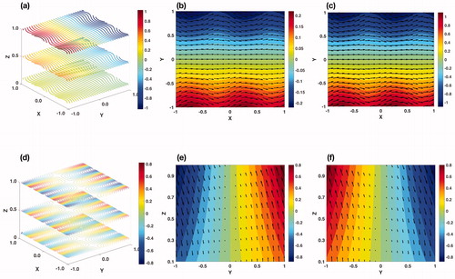
An important explicit example of non-zonal balanced flow is (54a) $$P_L=-(\Gamma +A\hspace{0.17em}\text{sin}\hspace{0.17em}\omega X)Yz$$(54a) (54b) $$u_L=(\Gamma +A\hspace{0.17em}\text{sin}\hspace{0.17em}\omega X)z$$(54b) (54c) $$v_L=-\mathit{\text{AωYz}}\hspace{0.17em}\text{cos}\hspace{0.17em}\omega X$$(54c) (54d) $$w_L=\frac{{\beta }_{L}A\omega }{H}Y\hspace{0.17em}\text{cos}\hspace{0.17em}\omega X\left(z+\frac{1}{H}\right)$$(54d) (54e) $${\Theta }_L=-(\Gamma +A\hspace{0.17em}\text{sin}\hspace{0.17em}\omega X)Y$$(54e) (54f) $$Q_L=\frac{{\beta }_{L}A\omega S}{H}Y\hspace{0.17em}\text{cos}\hspace{0.17em}\omega X\left(z+\frac{1}{H}\right),$$(54f) where we assume that H and S are positive constants. The above state is illustrated in Fig. 1. The balanced state is characterized by the zonal variability of baroclinicity, measured by meridional temperature gradient $\partial \Theta /\partial Y=-(\Gamma +A\hspace{0.17em}\text{sin}\hspace{0.17em}\omega X).$ If A and ω are small, v_L and w_L are both negligible. This basic state has been used to investigate the local baroclinic instability (Pierrehumbert, 1984). Figure 1(a) and (d) shows the zonal and meridional structure of the pressure P_L and thermal forcing Q_L on the three vertical levels. The zonal variability of baroclinicity originates from the zonally-varying force Q_L, which is reflected in potential temperature (colour) with geostrophic winds (arrows) in the surface (b) and an upper level (c). The zonally-varying pressure P_L leads to the nonzero meridional velocity v_L and the vertical velocity w_L, which is shown in (e) and (f) for two different X positions.

Fig. 1. The velocity, temperature and forcing associated with the pressure field, $P=-(\Gamma +A\hspace{0.17em}\text{sin}\hspace{0.17em}\omega X)Yz.$ The vertical and horizontal structure of P is shown in three representative vertical levels (a). The horizontal wind vector fields with streamlines in lower level (z = 0.1) and high level (z = 1.0) are shown in (b) and (c), respectively. The horizontal structures of the driving forcing Q_L are shown in the three vertical levels in (d). The meridional and vertical velocity with the forcing Q_L in Y – z plane is shown in (e) and (f), where two different X values are chosen as $X=-1.0$ (e) and X = 0 (f) and the colour represents the forcing Q_L.

Another example describes a balanced state where zonal-asymmetry, originated mainly from surface thermal forcing, disappears with height. This is closer to a realistic atmosphere. The example is (55a) $$P_L=-\Gamma Yz+A{e}^{-\gamma z}\hspace{0.17em}\text{sin}\hspace{0.17em}\omega$$(55a) (55b) $$u_L=\Gamma z$$(55b) (55c) $$v_L=-A\omega e^{-\gamma z}\hspace{0.17em}\text{sin}\hspace{0.17em}\omega X$$(55c) (55d) $$\Theta =-\Gamma Y-\gamma A{e}^{-\gamma z}\hspace{0.17em}\text{cos}\hspace{0.17em}\omega X$$(55d) (55e) $$w_L=\frac{{\beta }_{L}A\omega }{\gamma +H}{e}^{-\gamma z}\hspace{0.17em}\text{sin}\hspace{0.17em}\omega X$$(55e) (55f) $$\begin{array}{c}{Q}_L=\Gamma \omega A(1+\gamma z)e^{-\gamma z}\hspace{0.17em}\text{sin}\hspace{0.17em}\omega X\\ \hspace{1em}+\frac{S{\beta }_{L}A\omega }{\gamma +H}{e}^{-\gamma z}\hspace{0.17em}\text{sin}\hspace{0.17em}\omega X\\ \hspace{1em}+\frac{{\beta }_L\omega A^2{\gamma }^2}{\gamma +H}{e}^{-2\gamma z}\hspace{0.17em}\text{sin}\hspace{0.17em}\omega X\hspace{0.17em}\text{cos}\hspace{0.17em}\omega X.\end{array}$$(55f)

This is constructed by the given pressure (or streamline) P_L representing the sum of a zonal symmetric field $-\Gamma Yz$ and a zonal asymmetric one $A{e}^{-\gamma z}\hspace{0.17em}\text{sin}\hspace{0.17em}\omega X.$ The zonal asymmetric one is confined near the surface, which is described by the exponential decay with height. The zonal velocity u_L is only dependent upon z with the shear Γ and the meridional velocity v_L is concentrated near the surface. This state is illustrated in Fig. 2.

Fig. 2. Same as in Fig. 1 with the different pressure field $P=-\Gamma Yz+A{e}^{-\gamma z}\hspace{0.17em}\text{sin}\hspace{0.17em}(\omega X).$

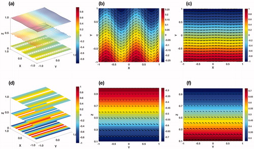
Figure 2(a) depicts the pressure fields on three vertical levels, showing the decrease of zonal asymmetry with height. The potential temperature (colour) and velocities (arrows) on surface (b) and on an upper level (c) are also shown. The zonal asymmetry identified by ‘wavy’ patterns on the surface diminishes almost entirely in upper levels. The relevant thermal forcing Q_L also decreases exponentially with height (d), implying that it is only influential near the surface. Figure 2(e) and (f) shows the meridional and vertical velocities on cold and warm surfaces, respectively. When the surface is cold (warm), wind takes downward (upward) and poleward (equatorward) directions.

The above two examples are the solutions of the planetary geostrophic motion without the influence of QG scales. The balanced state is the energy source for the growth of QG eddies through the baroclinic instability. Thus, identifying a balanced state is crucial for a physical interpretation of the statistics of geostrophic eddies in the atmosphere. For example, in the Northern hemisphere, land–sea contrast is one of the major factors controlling the spatial distribution of geostrophic eddies. Hence, it should be possible to initialize a numerical calculation of a balanced state with the thermodynamic forcing induced by the land–sea contrast, which could reveal the role of zonal asymmetry from the land–sea contrast on the baroclinic growth of synoptic waves and its feedback to the balanced state.

5. Discussion

Large-scale atmospheric dynamics is controlled by processes of different scales and the interactions between them. Unravelling the interactions – and ultimately understanding the dynamics in full – requires a systematic approach. In this paper, we have used an asymptotic approach to identify two separate scales in large-scale atmospheric dynamics and to understand the mutual interactions between them. Multi-scale analysis, in particular, is used in spatial and temporal domains to elucidate the interactions.

The two scales are distinguished by noting how the thermodynamic variables are scaled by the Rossby number ϵ. These variables are scaled by a length scale given by the meridional temperature gradient $\Delta T$ and the averaged surface temperature T₀. Two important parameters in this work, ϵ and $\alpha \equiv \Delta T/T_0,$ are related by $\alpha =Fϵ,$ where F is the inverse Burger number. When α is scaled by ${ϵ}^2,$ the O(1) equations reflect the geostrophic and hydrostatic balances, wherein the continuity and heat equations are automatically satisfied. However, at this order, the equations are degenerate and a unique solution is not available. To construct a closed equation set, we have considered the order $O(ϵ),$ which leads to the QG vorticity equation: this is the classic equation explaining the development and saturation of synoptic waves, essential to weather phenomena. In contrast, when α is scaled by ϵ, the continuity and heat equations survive at the leading order. The former simplifies to the ‘Sverdrup relation’, and the latter governs the evolution of the main dynamics. Here, a given large-scale thermodynamic forcing can lead to a unique state satisfying the hydrostatic and geostrophic balances – the state of PG motion.

In this work, we have argued that the variation and structure of the large-scale atmospheric motion can be viewed in terms of the interaction of two geostrophic motions. One motion, the PG motion, can be interpreted as a balanced field directly forced by large-scale radiative-convective imbalance, as just noted, and the other motion, aptly descried by the familiar QG vorticity equation, governs the life cycle of synoptic waves that grow via the energy extracted from the balanced field.

The interaction is systematically revealed in a multi-scale analysis, in which the PG motion provides the mean field in the QG vorticity equation. The mean field provides the background condition, for example, for the growth of QG perturbations. It is important to note that baroclinic instability problems studies thus far have mainly employed zonally-symmetric flow with vertical shear represented often with a simple linear dependence with height. However, such a setup is not realistic. Our approach affords a generalisation of the traditional baroclinic instability study (cf., Figs. 1 and 2), by permitting the instability to be directed connected to the large-scale heat flux imbalance. Such connection may be significant in the current discussion about the impact of global warming on the weather.

Another significant perspective addressed through the multi-scale analysis is the construction of a statistically-stationary large-scale flow – i.e. PG motion forced by both the large-scale radiative imbalance and the QG eddies. Averaging the QG variables in time domain shows the contribution of the QG motion to the slow time evolution of the PG motion. The time-averaged horizontal heat flux convergence and vertically-integrated relative vorticity flux convergence act as forcing in the planetary heat equation. Then, the PG motion is balanced by the radiative imbalance and the heat and vorticity flux convergences. The mutual interaction of the two scales discussed in this work extended the study by Dolaptchiev and Klein (2013), in which the PG and the QG are connected solely through the time evolution of the barotropic component of background pressure.

Acknowledgements

W.M. acknowledges a Herchel-Smith postdoctoral fellowship. This work was initiated at the 2015 Geophysical Fluid Dynamics Summer Study Program ‘Stochastic Processes in Atmospheric & Oceanic Dynamics’ at the Woods Hole Oceanographic Institution, which is supported by the National Science Foundation and the Office of Naval Research. W.M also acknowledges the support of Swedish Research Council grant no. 638-2013-9243. J.Y-K.C. acknowledges the hospitality of the Kavli Institute for Theoretical Physics, Santa Barbara and the Department of Astrophysical Sciences, Princeton University, where some of this work was completed. We are grateful to Joe Pedlosky for very helpful discussions and comments.

Disclosure statement

No potential conflict of interest was reported by the authors.

Additional information

Funding

W.M. also acknowledges Swedish Research Council grant no. 638-2013-9243 for support. This research was supported in part by the National Science Foundation under Grant No. NSF PHY-1748958.

References

- Chang, E. K., Lee, S. and Swanson, K. L. 2002. Storm track dynamics. J. Clim. 15, 2163–2183. doi:10.1175/1520-0442(2002)015<02163:STD>2.0.CO;2
- Charney, J. G. 1947. The dynamics of long waves in a baroclinic westerly current. J. Meteor. 4, 136–162. doi:10.1175/1520-0469(1947)004<0136:TDOLWI>2.0.CO;2
- Dolaptchiev, S. I. and Klein, R. 2009. Planetary geostrophic equations for the atmosphere with evolution of the barotropic flow. Dyn. Atmos. Oceans 46, 46–61. doi:10.1016/j.dynatmoce.2008.07.001
- Dolaptchiev, S. I. and Klein, R. 2013. A multiscale model for the planetary and synoptic motions in the atmosphere. J. Atmos. Sci. 70, 2963–2981. doi:10.1175/JAS-D-12-0272.1
- Eady, E. T. 1949. Long waves and cyclone waves. Tellus A 1, 33.
- Held, I. M. 1983. Stationary and quasi-stationary eddies in the extratropical troposphere: theory. In: Large-Scale Dynamical Processes in the Atmosphere (eds. B. Hoskins and R. P. Pearce), Academic Press, New York, 127–168 pp.
- Held, I. M. and Suarez, M. J. 1994. A proposal for the intercomparison of the dynamical cores of atmospheric general circulation models. Bull. Amer. Meteor. Soc. 75, 1825–1830. doi:10.1175/1520-0477(1994)075<1825:APFTIO>2.0.CO;2
- Held, I. M., Pierrehumbert, R. T., Garner, S. T. and Swanson, K. L. 1995. Surface quasi-geostrophic dynamics. J. Fluid Mech. 282, 1–20. doi:10.1017/S0022112095000012
- Leathers, D. J., Yarnal, B. and Palecki, M. A. 1991. The Pacific/North American teleconnection pattern and United States climate. Part I: regional temperature and precipitation associations. J. Clim. 4, 517–528. doi:10.1175/1520-0442(1991)004<0517:TPATPA>2.0.CO;2
- Marshall, J., Kushnir, Y., Battisti, D., Chang, P., Czaja, A. and co-authors. 2001. North Atlantic climate variability: phenomena, impacts and mechanisms. Int. J. Climatol. 21, 1863–1898. doi:10.1002/joc.693
- Polvani, L. M., Scott, R. K. and Thomas, S. J. 2004. Numerically converged solutions of the global primitive equations for testing the dynamical core of atmospheric GCMs. Mon. Wea. Rev. 132, 2539–2552. doi:10.1175/MWR2788.1
- Pedlosky, J. 2013. Geophysical Fluid Dynamics. Springer Science & Business Media, New York, 336 pp.
- Phillips, N. A. 1954. Energy Transformations and Meridional Circulations associated with simple Baroclinic Waves in a two-level, Quasi-geostrophic Model. Tellus A 6, 273–286. doi:10.1111/j.2153-3490.1954.tb01123.x
- Phillips, N. A. 1963. Geostrophic motion. Rev. Geophys. 1, 123–176. doi:10.1029/RG001i002p00123
- Pierrehumbert, R. T. 1984. Local and global baroclinic instability of zonally varying flow. J. Atmos. Sci. 41, 2141–2162. doi:10.1175/1520-0469(1984)041<2141:LAGBIO>2.0.CO;2
- Schneider, T. 2006. The general circulation of the atmosphere. Annu. Rev. Earth Planet. Sci. 34, 655–688. doi:10.1146/annurev.earth.34.031405.125144
- Simmons, A. J. and Hoskins, B. J. 1977. Baroclinic instability on the sphere: solutions with a more realistic tropopause. J. Atmos. Sci. 34, 581–588. doi:10.1175/1520-0469(1977)034<0581:BIOTSS>2.0.CO;2
- Simmons, A. J. and Hoskins, B. J. 1978. The life cycles of some nonlinear baroclinic waves. J. Atmos. Sci. 35, 414–619. doi:10.1175/1520-0469(1978)035<0414:TLCOSN>2.0.CO;2
- Sverdrup, H. U. 1947. Wind-driven currents in a baroclinic ocean; with application to the equatorial currents of the eastern Pacific. Proc. Natl. Acad. Sci. 33, 318–326. doi:10.1073/pnas.33.11.318
- Welander, P. 1959. An advective model of the ocean thermocline. Tellus A 11, 309–318.