Assimilation of semi-qualitative sea ice thickness data with the EnKF-SQ: a twin experiment

Abstract

A newly introduced stochastic data assimilation method, the Ensemble Kalman Filter Semi-Qualitative (EnKF-SQ) is applied to a realistic coupled ice-ocean model of the Arctic, the TOPAZ4 configuration, in a twin experiment framework. The method is shown to add value to range-limited thin ice thickness measurements, as obtained from passive microwave remote sensing, with respect to more trivial solutions like neglecting the out-of-range values or assimilating climatology instead. Some known properties inherent to the EnKF-SQ are evaluated: the tendency to draw the solution closer to the thickness threshold, the skewness of the resulting analysis ensemble and the potential appearance of outliers. The experiments show that none of these properties prove deleterious in light of the other sub-optimal characters of the sea ice data assimilation system used here (non-linearities, non-Gaussian variables, lack of strong coupling). The EnKF-SQ has a single tuning parameter that is adjusted for best performance of the system at hand. The sensitivity tests reveal that the tuning parameter does not critically influence the results. The EnKF-SQ makes overall a valid approach for assimilating semi-qualitative observations into high-dimensional nonlinear systems.

Keywords:

• semi-qualitative observations
• range limitation
• SMOS
• ice thickness
• TOPAZ4
• EnKF-SQ

1. Introduction

Sea ice plays a crucial role in the Arctic climate as it modulates the exchange of heat and moisture between the ocean and the atmosphere (Aagaard and Carmack, 1989; Screen and Simmonds, 2010). Different studies have shown that accurate knowledge of the Sea Ice Thickness (SIT) is beneficial for the Arctic sea ice predictability (Day et al., 2014; Guemas et al., 2016; Collow et al., 2015). The SIT observations from the European Space Agency (ESA) Soil Moisture and Ocean Salinity (SMOS) mission are available in near-real time, at daily frequency during the cold season (October-April). The retrieval method for SMOS SIT observations is based on measurements of the brightness temperature at a low frequency microwave (1.4 GHz, L-band: wavelength of 21 cm) (Kaleschke et al., 2010). The representative depth for the L-Band microwave frequency into the sea ice is about 0.5 m for first-year level ice (Kaleschke et al., 2010; Huntemann et al., 2014). After an initial study indicating a limit at 0.5 m, Tian-Kunze et al. (2014) developed a novel iterative retrieval algorithm for SMOS SIT observation, that is based on a thermodynamic sea ice model and three-layer radiative transfer model, which explicitly takes variations of ice temperature and ice salinity into account. The newly developed algorithm can estimate the ice thickness up to maximum of 1 m depending on the ice temperature and salinity. Few studies have shown that assimilating thin SIT from SMOS into coupled ice-ocean model, using ensemble based Data Assimilation (DA) techniques, is able to improve the SIT forecast without being detrimental to other properties (e.g. Yang et al., 2014; Xie et al., 2016; Fritzner et al., 2019). All of these studies, however, ignore the saturated observations of thick ice.

Measurements of thick sea ice on basin-wide scales are also available from laser altimeters onboard ICESat (Forsberg and Skourup, 2005) or from radar altimeters on the European Remote Sensing (ERS), Envisat, CryoSat-2 and Sentinel-3 (Connor et al., 2009; Laxon et al., 2013; Ricker et al., 2014). CryoSat-2 SIT is provided in near-real time (Tilling et al., 2016) but still contains considerable large uncertainties caused by the lack of auxiliary data on snow depth. These uncertainties are proportionally larger for thin ice (i.e. <1 m) and hence CryoSat-2 practically measures thick sea ice only. A merged product of weekly SIT observations in the Arctic from the CryoSat-2 altimeter and SMOS radiometer, referred as CS2SMOS, has also been developed by combining the two complementary datasets (Kaleschke et al., 2015; Ricker et al., 2017) and made available during the winter months since October 2010. However, the combination of the two satellites is not perfect as biases have been revealed on overlapping areas (Wang et al., 2016; Ricker et al., 2017). Recently, Xie et al. (2018) successfully assimilated the merged SIT product CS2SMOS into the TOPAZ4 coupled ocean-sea ice reanalysis system (Sakov et al., 2012) for the Arctic.

While assimilating a merged SIT map, rather than two satellites data streams is practically convenient, the uncertainty of the merged data is more difficult to quantify and bad quantification of the uncertainty may affect the assimilation performance negatively (Mu et al., 2018).¹ The ability to use well-justified observation errors in data assimilation is sufficiently important to motivate the assimilation of the two separate SIT data streams rather than one merged product. This implies that their detection limits should be taken into account by the data assimilation method.

In DA, observations are used to reduce the error of the state variables so that the forecast skill can be enhanced. Many observations can only be retrieved within a limited interval of the values that the observed quantity would take in nature. In other words, observations may have a detection limit. One such example is the aforementioned observation of SIT from SMOS. Although, the SIT observations with detection limit do not provide quantifiable data (hard data) above its detection limit, they do give qualitative information (soft data). For instance, the ice could be thicker than a known threshold. Studies from Shah et al. (2018) and Borup et al. (2015) have shown that assimilating soft data with linear and non-linear toy models using ensemble-based DA methods have the potential to improve the accuracy of the forecast. Therefore, not considering soft data in the assimilation procedure is a potential loss of meaningful information.

Assimilating only thin ice observations, as in Xie et al. (2016, figures 5 and 6), induces a low bias, which is caused by the partial nature of the observation of thin ice. With a new method intended for semi-qualitative data as the EnKF-SQ, the question arise whether this bias can be mitigated or not? The comparison of the EnKF-SQ to the perfect Bayesian solution (Shah et al., 2018) shows that the EnKF-SQ analysis does not coincide with the Bayesian posterior and bears inherent biases: in the case of hard data, the Bayesian and EnKF-SQ posteriors are nearly the same. However, for out-of-range observations and mode of a prior within the observable range, only the maximum likelihood of the EnKF-SQ analysis is preserved but its distribution is flatter than the Bayesian solution with a thicker tail in the unobservable range, so the expectation is too high. Based on this, the EnKF-SQ is expected to be unbiased for thin SIT observations. Nevertheless, it should show a positive bias for out-of-range observations. Further, the thicker tail of the EnKF-SQ analysis distribution in the unobservable range makes it relatively skewed, which is undesirable in a Kalman filtering context.

In this study, we implement and test the overall performance of the stochastic ensemble Kalman filter semi-qualitative (EnKF-SQ) (Shah et al., 2018) in a twin experiment where synthetic SMOS-like SIT observations, with an upper detection limit, are assimilated into a coupled ocean-sea ice forecasting system. The objective is to test the potential of the EnKF-SQ for assimilating soft data within a state of the art ocean and sea ice prediction system, namely TOPAZ4. In addition, a number of single-cycle assimilation experiments using the EnKF-SQ are performed to investigate the sensitivity to the ensemble size and out-of-range observation uncertainty.

This paper is organized as follows: Section 2 introduces the main components of the TOPAZ4 system including the model and the EnKF-SQ DA scheme used in the assimilation experiments. In Section 3, the synthetic ice thickness data are outlined together with the assimilation setup. Section 4 discusses the results of the various assimilation experiments. A general discussion of the study concludes the paper in Section 5.

2. The TOPAZ system

2.1. Model setup

The ocean general circulation model used in the TOPAZ4 system is the version 2.2 of the Hybrid Coordinate Ocean Model (HYCOM) developed at the University of Miami (Bleck, 2002; Chassignet et al., 2003). The TOPAZ4 implementation of HYCOM uses hybrid coordinates in the vertical, which smoothly shift from isopycnal layers in the stratified open ocean to z level coordinates in the unstratified surface mixed layer.

The HYCOM ocean model is coupled to a one-thickness category sea ice model. The single ice thickness category thermodynamics are described in Drange and Simonsen (1996) and the ice dynamics use the Elastic-Viscous-Plastic (EVP) rheology of Hunke and Dukowicz (1997) with a modification from Bouillon et al. (2013). The momentum exchange between the ice and the ocean is given by quadratic drag formulas. The model has a minimum thickness of 10 cm for both new and melting ice.

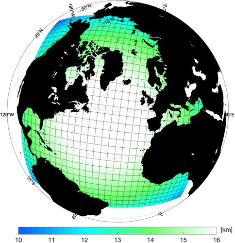
The model domain covers the Arctic and North Atlantic basins as shown in Fig. 1. The model grid is created with conformal mapping (Bentsen et al., 1999) and has a quasi-homogeneous horizontal resolution between $12-16$ km in the whole domain. The grid has 880 × 800 horizontal grid points.

Fig. 1. The TOPAZ4 model domain. Background color shading shows the horizontal grid resolution (km) while solid black color represents land.

2.2. The ensemble Kalman filter semi-qualitative, EnKF-SQ

The EnKF-SQ (Shah et al., 2018) uses an ensemble of model states to estimate the error statistics closely following the stochastic EnKF algorithm (Burgers et al., 1998; Evensen, 2004). The stochastic EnKF is a two-step filtering method alternating forecast and analysis steps. In the forecast step, the ensemble of model states is integrated forward in time and when observations become available, an analysis of every forecast member, ${\mathbf{x}}_i^f$ for $i\in 1,2,\dots ,N,$ is computed as follows: (1) $${\mathbf{x}}_i^a={\mathbf{x}}_i^f+\mathbf{K}({\mathbf{y}}_i-\mathbf{H}{\mathbf{x}}_i^f),$$(1) (2) $$\mathbf{K}={\mathbf{P}}^f{\mathbf{H}}^T{(\mathbf{H}{\mathbf{P}}^f{\mathbf{H}}^T+\mathbf{R})}^{-1},$$(2) where K is the Kalman gain matrix; ${\mathbf{x}}_i$ is the ith ensemble state member; H is the observation operator, mapping the state variable to the observation space (could be non-linear); R is the observation error covariance matrix; ${\mathbf{y}}_i$ is the ith perturbed observation vector generated from $\mathcal{N}(\mathbf{y},\mathbf{R})$ and ${\mathbf{P}}^f$ is the ensemble forecast error covariance matrix. The superscripts a, f, and T stand for analysis, forecast, and matrix transpose, respectively. In practice, ${\mathbf{P}}^f$ is never computed explicitly and is instead decomposed as follows: (3) $${\mathbf{P}}^f=\frac{1}{N-1}\sum _{i=1}^N({\mathbf{x}}_i^f-{\overline{\mathbf{x}}}^f){({\mathbf{x}}_i^f-{\overline{\mathbf{x}}}^f)}^T,$$(3) where ${\overline{\mathbf{x}}}^f$ is the mean of the forecast ensemble.

The EnKF-SQ is intended to explicitly assimilate observations with a detection limit. These are divided into two categories depending on whether they are within or outside the observable range. If the observed quantity is within it, the quantitative (hard) data is assimilated as in the stochastic EnKF, otherwise it is considered a qualitative (soft) data and treated differently. The observation error std for hard data is a function of ice thickness as discussed below in Section 3.1.

The specific value and error statistics of the out-of-range (OR) observations are unknown. In order to assimilate OR observations, an assumption needs to be made about its likelihood. Following Shah et al. (2018), a virtual observation is created at the detection limit and then a two-piece Gaussian observation likelihood is constructed around it. A two-piece Gaussian distribution is obtained by merging two opposite halves of two different Gaussian probability density functions (pdfs) at their common mode, given as follows: (4) $$f(x)=\{\begin{array}{c}w{e}^{-{\left(x-\mu \right)}^2/2{\sigma }_{ir}^2},x\le \mu ,\hfill \\ w{e}^{-{\left(x-\mu \right)}^2/2{\sigma }_{or}^2},x>\mu ,\hfill \end{array}$$(4) where $w=\sqrt{\frac{2}{\pi }}{({\sigma }_{ir}+{\sigma }_{or})}^{-1}$ is a normalizing constant, μ is the detection limit and also the common mode of two different normal distribution; σ_ir and σ_or are in-range and OR observation error standard deviations (std), respectively.

Figure 2 is an illustration of a two-piece Gaussian observation likelihood for OR SIT observations. On the left hand side of the detection limit, it is assumed that σ_ir, inside the observable range, is defined by the observation uncertainty of hard data at the detection limit. This is because an observation could possibly fall outside the detection limit, due to observation errors, even though its true value is within the observable range. On the right hand side, it is assumed that the σ_or (Eq. 5(5) $${\sigma }_{or}=\underset{}{\underset{\text{Climatological}\text{mean}}{\underbrace{\underset{\mu }{\overset{+\infty }{\int }}y{f}_c(y)dy}}}-\mu .$$(5) ) in the unobservable range is defined with the help of a climatological mean for SIT above the detection limit so that extremely high values, which are usually less realistic, receive a lower likelihood (Shah et al., 2018). (5) $${\sigma }_{or}=\underset{}{\underset{\text{Climatological}\text{mean}}{\underbrace{\underset{\mu }{\overset{+\infty }{\int }}y{f}_c(y)dy}}}-\mu .$$(5)

Fig. 2. Illustration of the two-piece Gaussian OR-observation likelihood for SMOS-like thin SIT. σ_ir is an in-range and σ_or is the out-of-range observation error standard deviations, respectively.

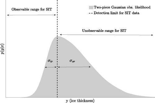
$f_c(y)$ is the pdf of the climatological data of the observed quantity. The two-piece Gaussian observation likelihood for soft data is denoted, hereafter, by ${\mathcal{N}}_{2p}(\mu ,{\sigma }_{ir}^2,{\sigma }_{or}^2).$ The EnKF-SQ pre-processes the observations by sorting them as either hard y^h or soft y^s. The observation errors are assumed uncorrelated in space, i.e. R is diagonal.

Update step of the EnKF-SQ

For each forecast member ${\mathbf{x}}_i^f$ ($i\in 1,2,\dots ,N$):

1. For each soft data $y_j^s,$ check whether the observed forecast ensemble member is within the observable range or not.

2. If ${\mathbf{H}}_j{\mathbf{x}}_i^f\le \mu ,$ set observation error variance ${\mathbf{R}}_{j,j}={\sigma }_{ir}^2$ otherwise ${\mathbf{R}}_{j,j}={\sigma }_{or}^2$ implying that members inside (outside) the observable range are updated with data parameterized using in-range ${\sigma }_{ir}^2$ (out-of-range ${\sigma }_{or}^2$).

3. After looping over all soft data, compute the Kalman gain ${\mathbf{K}}_i$ as in Eq. 2(2) $$\mathbf{K}={\mathbf{P}}^f{\mathbf{H}}^T{(\mathbf{H}{\mathbf{P}}^f{\mathbf{H}}^T+\mathbf{R})}^{-1},$$(2) with the updated observation error covariance matrix R. For each ${\mathbf{x}}_i^f,$ a different Kalman gain ${\mathbf{K}}_i$ is calculated.

4. Evaluate the $i^{\text{th}}$ analysis member ${\mathbf{x}}_i^a$ as in Eq. 1(1) $${\mathbf{x}}_i^a={\mathbf{x}}_i^f+\mathbf{K}({\mathbf{y}}_i-\mathbf{H}{\mathbf{x}}_i^f),$$(1) using ${\mathbf{K}}_i.$ The perturbed observations are generated by sampling from $\mathcal{N}(y_j^h,{\sigma }_h^2)$ and ${\mathcal{N}}_{2p}(\mu ,{\sigma }_{ir}^2,{\sigma }_{or}^2)$² for $y_j^h$ and $y_j^s,$ respectively. ${\sigma }_h^2$ is the observation error variance for $y_j^h.$

Loop to next member i.

Repeating this process for all forecast members yields the analysis ensemble. For a detailed description of the EnKF-SQ, the reader is referred to Section 2 of Shah et al. (2018).

3. Experimental setup

3.1. The synthetic sea ice thickness data

The synthetic SIT data used in this study is intended to mimic the SIT data from the SMOS mission with an upper detection limit. In order to evaluate the EnKF-SQ method against a perfectly known truth, synthetic observations are generated using the coupled ocean and one-thickness category sea ice model described earlier in Section 2.1. A reference truth run (also called nature run) is produced by integrating the coupled ocean sea ice model from 1 January, 2014 to 31 December, 2015 using unperturbed atmospheric forcing from ERA-Interim (Dee et al., 2011). The run is initialized using member number 100 from the 100-member ensemble reanalysis of Xie et al. (2017) on 31 December, 2013.

Synthetic SIT data are then generated for the duration of the assimilation experiment from 11 November 2014 to 31 March 2015 by perturbing the truth with Gaussian noise of zero mean and standard deviation σ_obs; parameterized as: (6) $${\sigma }_{\mathit{obs}}=0.06t+0.05,$$(6) where t is the truth for ice thickness in meters. The parameterization is chosen such that observation errors increase for thicker ice, which is a general behaviour of positive-valued variables like SIT. The relationship is obtained through regression of the absolute difference of the daily averaged SIT between the aforementioned reference trajectory and reanalysis product (Xie et al., 2017) on the reference truth from the month of December 2014 to January 2015. The resulting relationship (not shown here) is linear with a positive slope. SIT observation error represented in Eq. 6(6) $${\sigma }_{\mathit{obs}}=0.06t+0.05,$$(6) is also qualitatively in line with those used by Xie et al. (2016) for SMOS data.

In order to avoid any ambiguity and to have a simplified case of SMOS SIT detection limit, a single upper detection limit of 1 m is imposed on the generated SIT observations, as an analogous for saturation of SMOS data in thick sea ice. The SIT observations are assumed available on every grid cell (except along the coastline) and assimilated on a weekly basis. This is a reasonable assumption as SMOS data comes with a grid resolution of ($\sim 12.5$ km), which is also the resolution of the TOPAZ4 system. Model and observation grids are collocated, thus our experiments neglect potential errors due to interpolation, which is out of the scope of this study.

3.2. Out-of-range SIT climatology

A trivial alternative to the EnKF-SQ in the presence of soft data would be to assimilate climatological data as hard data. It is, therefore, worth investigating how beneficial the assimilation of soft data with the EnKF-SQ is compared to assimilating climatology.

The Arctic sea ice being in a declining phase, a climatology of sea ice thickness represents a moving target. In order to construct a climatology that is not drastically off the conditions of the present experiment, we selected one pragmatic compromise: a short two-year average from 2014 to 2015, which covers the experiment period and hence gives a relatively accurate climatology. An out-of-range, location-dependent, yearly SIT climatology is computed by taking a time average of the truth (described earlier) for SIT above the detection limit in each grid cell. Averaging is done from January 2014 to December 2015, a period that includes two summers and two winters and encompasses the assimilation period. Even though the latter takes place in winter, the climatology has a high bias because by construction it only contains SIT above 1 m. The observation error variance for the climatological value is also location-dependent, equal to the variance of all reference truth values above the detection limit in the same grid cell.

3.3. Assimilation setup

In contrast to earlier TOPAZ4 studies that updated the whole water column variables (Xie et al., 2018), here the state vector x consists of only two sea ice variables: SIT and sea ice concentration (SIC). This therefore constitutes a case of a weakly coupled assimilation where the ocean is only updated by dynamical re-adjustments from the sea ice updates. Kimmritz et al. (2018), have shown that while strongly coupled ocean and sea ice is clearly beneficial, weakly coupled DA can still achieve reasonable results.

In the analysis, sampling errors in the forecast error covariance can give rise to spurious correlations between remote grid points, a problem which may become more pronounced for smaller ensemble sizes (Houtekamer and Mitchell, 1998). A common practice to counteract sampling errors is to perform local analysis in which variables at each grid cell are updated using only the observations within a radius of influence r_o around the grid cell (Houtekamer and Mitchell, 1998; Evensen, 2003). For simplicity, a single closest local observation within r_o = 300 km is used here during the analysis.

In TOPAZ4, model error is introduced by increasing the model spread via perturbing few forcing fields. The perturbations are pseudo-random fields computed in a Fourier space with a decorrelation time-scale of 2 days and horizontal decorrelation length scale of 250 km, as described in Evensen (2003). Perturbed variables include air temperature, wind speeds, cloud cover, sea level pressure (Sakov et al., 2012, Section 3.3) and yield curve eccentricity in the EVP rheology (Hunke and Dukowicz, 1997, table 1). In addition, precipitation is also perturbed with log-normal noise and standard deviation of 100%. This affects the snowfall when temperatures are below zero. Snow is an important thermal insulator and therefore hampers sea ice growth/melt.

3.4. Target benchmarks

The performance of the EnKF-SQ is compared against three different versions of the stochastic EnKF and a Free run, denoted as follows:

1. EnKF-ALL: No detection limit is applied on SIT observations thus even thick ice data from the reference run is assimilated. This run acts as an upper bound for performance because it is the only one that assimilates out-of-range observations as hard data with known statistics, which can be seen as cheating.

2. EnKF-CLIM: The SIT climatology with climatological variance is assimilated instead of soft data.

3. EnKF-IG: Only hard data is assimilated and soft data is ignored, similar to Xie et al. (2016). This run is meant to assess the added value of the EnKF-SQ.

4. Free-run: The Free-run is the average of the 99 members without DA. It is run with perturbations, contrarily to the aforementioned single-member truth run.

To evaluate the performance of the different DA methods, we compute the root mean square error (RMSE) of the ensemble mean at time t as: (7) $${\text{RMSE}}_t=\sqrt{\frac{1}{n}\sum _{i=1}^n{\left({\overline{\mathbf{x}}}_{i,t}^f-{\mathbf{x}}_{i,t}^r\right)}^2},$$(7) where ${\mathbf{x}}^r$ and ${\overline{\mathbf{x}}}^f$ is the n-dimensional reference (unperturbed truth) and mean of the prior state vector at time t, respectively. We also monitor the average ensemble spread (AES) for each filter, which we calculate at every assimilation cycle as: (8) $${\text{AES}}_t=\sqrt{\frac{1}{n}\sum _{i=1}^n{\sigma }_{i,t}^2},$$(8) where ${\sigma }_{i,t}^2$ can either be the prior or posterior ensemble variance at time t, respectively.

3.5. Ensemble size

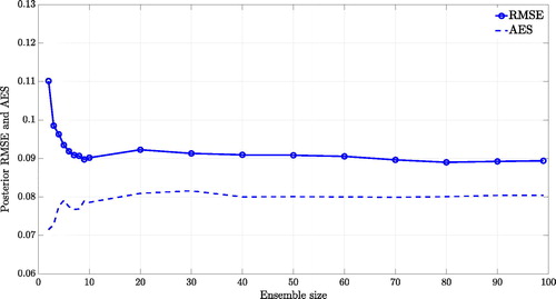
In order to select the ensemble size, single-cycle assimilation sensitivity experiments are conducted using EnKF-SQ by varying the ensemble size between 2 and 99. The resulting time-averaged RMSE and AES of the posterior SIT estimates are displayed in Fig. 3. The plot indicates that for $N\ge 10,$ there is no significant difference in the performance of the EnKF-SQ. This is mostly due to the small size of the local state vector; consisting only of two variables. An ensemble as small as 10 members is however less likely to succeed on the long term especially if the number of state variable and observations increase. Results from the other three EnKF runs (not shown) showed the exact same behavior. Thus, the initial ensemble is set as the first 99 members of the reanalysis ensemble of Xie et al. (2016) on 31 December 2013. The initial ensemble is then spun up from January, 2014 until the start of the assimilation experiment (i.e. November 11) with perturbed forcing to increase the variability. As described earlier, member number 100 of the reanalysis run was used to generate the truth in this study.

Fig. 3. Time-averaged posterior RMSE and AES resulting from single cycle assimilation runs for different ensemble sizes using EnKF-SQ.

The assimilation framework is sub-optimal for few reasons, in particular because of the weakly coupled updates. Further, SIT errors are erroneously assumed Gaussian while they are not. These sub-optimalities are not uncommon in realistic applications. They do cause some limited loss of performance but generally do not prevent us from applying the EnKF.

In terms of computational resources, we used a single processor on supercomputer for each of the four DA methods. The total wall-clock time required by each analysis scheme, to update the SIT and SIC state variables along with the IO operations, is approximately 6 minutes on a 1.4 GHz Cray XE6. This is much less than the TOPAZ4 one-week forward model run, for which each member runs on 134 parallel processors in approximately 5 minutes.

4. Assimilation results

4.1. Tuning the EnKF-SQ out-of-range likelihood

The out-of-range standard deviation σ_or is the only new parameter introduced into the EnKF-SQ compared to the stochastic EnKF. Therefore, it is important to study how the uncertainty in the estimate of σ_or affects the performance of the EnKF-SQ scheme. For this, we carried out a number of single-cycle assimilation experiments by introducing a scalar multiplier α to Eq. 5(5) $${\sigma }_{or}=\underset{}{\underset{\text{Climatological}\text{mean}}{\underbrace{\underset{\mu }{\overset{+\infty }{\int }}y{f}_c(y)dy}}}-\mu .$$(5) such that ${\sigma }_{or}^{*}=\alpha ·{\sigma }_{or}.$

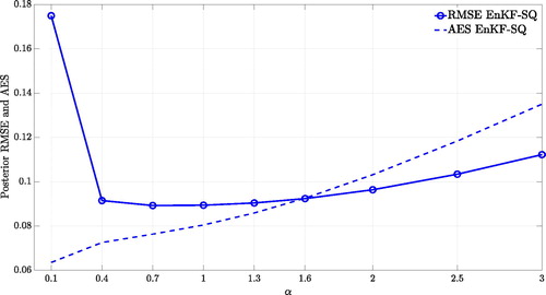
RMSE and AES of the posterior SIT estimates are plotted in Fig. 4 for a wide range of α, varying between 0.1 and 3.0. Such a range is very broad for most realistic applications. $\alpha <0.4$ strongly degrades the accuracy of the EnKF-SQ along with significant decrease in the AES. The large difference between RMSE and AES values, indicate a possible filter divergence. This is because for small α values, the sampling of a two-piece Gaussian likelihood for observation perturbations is prone to generate samples concentrated around the detection limit, thus pulling the analysis close to the detection limit, subsequently reducing the ensemble spread and increasing the RMSE. As α approaches 1, the RMSE attains the minimum value and further becomes consistent with the AES. When α increases beyond 2, large random samples are occasionally drawn from the wide (fat tail) two-piece OR likelihood and large perturbations are propagated to the state vector through the Kalman gain, which eventually deteriorates the performance of the EnKF-SQ (with larger analysis RMSE). Accordingly, in what follows we set α = 1.

Fig. 4. Time-averaged posterior RMSE and AES resulting from single cycle assimilation runs for a wide range of the multiplicative factor α.

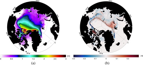
To illustrate how the EnKF-SQ updates the SIT by assimilating range-limited SIT observations, we plot the prior mean (Fig. 5a) and analysis increment (Fig. 5b) on 11 November 2014. The solid black line on both maps is the isoline for 1 m of SIT. The forecast places the thick ice (up to 3 m) north of Greenland and north-eastern part of Canada. The increments are not only visible outside of the 1 m isoline but also inside the central Arctic region where only soft data are assimilated. It is important to notice that there is nearly zero increment in the central Arctic region and the Beaufort sea where the sea ice is thicker than 1.5 m. This is because the EnKF-SQ analysis do not impose strong updates on the prior if it is above the detection limit and observations are out-of-range.

Fig. 5. (a) Prior ensemble mean of the ice thickness on 11 November 2014. The solid black line is the 1 m SIT isoline. (b) The increment (analysis-forecast) for SIT after incorporating the observations.

4.2. Performance assessment

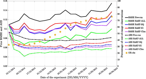
Figure 6 shows the time evolution of the RMSE and AES of the prior SIT estimates obtained using the EnKF-ALL, EnKF-SQ, EnKF-CLIM, EnKF-IG and the Free-run. The percentage of OR observations (to the total number of observations) available at every cycle is added to the plot. As expected, EnKF-ALL outperforms all other schemes while EnKF-IG is the least accurate. It should be noted that there is an increasing trend in the RMSE, which is seasonally driven; a similar behavior reported in Xie et al. (2016). Assimilating soft data with the EnKF-SQ clearly improves the prior RMSE compared to the EnKF-IG. This is consistent over the entire assimilation period. The number of OR observations gradually increases as the cold season intensifies leaving only a few hard data during the months of February and March 2015. Even with a very limited number of hard data, the EnKF-SQ outperforms EnKF-IG. On average the EnKF-SQ improves the forecast accuracy by approximately 8% compared to the EnKF-IG. The RMSE resulting from the EnKF-CLIM is marginally higher than that of the EnKF-SQ, except during the last three months of the assimilation experiment. The reason for this could be twofold: (i) In the early stages of the experiment, the climatology tends to overestimate SIT due to the large seasonal cycle compared to later months. This causes the climatology to pull the update towards large values and hence degrades the performance of the EnKF-CLIM. (ii) Fewer hard data leads to larger RMSE values in the EnKF-SQ as can be seen towards the end of winter and start of the spring. Overall, the RMSE and AES show consistent ensemble statistics such that sufficient variability is preserved in the system after cycling over time.

Fig. 6. Left y-axis: Time evolution of the prior RMSE (solid lines) and AES (dashed lines) for SIT estimates. Right y-axis: The orange asterisks represent the percentage of the out-of-range observations during assimilation resulting from the EnKF-SQ, EnKF-CLIM and EnKF-IG.

In order to visualize area-wise improvements, we plot the map of time-averaged RMSE of the SIT prior estimates in Fig. 7. The EnKF-ALL yields the best RMSE throughout the entire region. Compared to the EnKF-IG, the EnKF-SQ performs better in the central Arctic region, Greenland’s north-eastern shelf, the Canadian Arctic Archipelago and in the Beaufort Sea. On average, the EnKF-SQ and EnKF-CLIM estimates are approximately 8% more accurate than those of the EnKF-IG.

Fig. 7. Maps of time-averaged prior RMSE for SIT obtained using: EnKF-ALL (top left), EnKF-SQ (top right), Free-run (center left), EnKF-CLIM (bottom left) and EnKF-IG (bottom right). Averaging is done over the period of experiment, i.e. from November 2014 to March 2015.

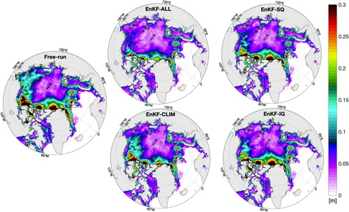
The EnKF-CLIM, seems to produce larger improvements than the EnKF-SQ specifically along the Ellesmere island. However, it also increases the prediction error in the Beaufort sea more than that of the EnKF-IG. A number of reasons may explain this behavior. The climatology being too high compared to the seasonal mean yields an artificial increase of the model thickness, which happens to agree with the truth along the Ellesmere island. The recurrent update due to the assimilation of climatology is propagated dynamically by the Beaufort gyre into the Beaufort sea creating an anomaly compared to the truth, which is not thicker.

The analysis algorithm of the EnKF-SQ is designed such that improvements are expected mostly where SIT is close to the threshold. As a way to examine this, we computed the time-averaged RMSE of the prior SIT estimates for different ice thickness intervals of 25 cm using all DA schemes (Fig. 8). The values on the x-axis of Fig. 8 represent the upper bounds of each 25 cm SIT bin interval except for the first bin of size 10 cm because of the model 10 cm minimum thickness. The RMSE for all DA schemes within each SIT bin is computed by finding the location of grid cells for which the observations fall within the bin interval.

Fig. 8. Bar chart of time-averaged conditional prior RMSEs for SIT obtained using all tested DA schemes. Solid black line represents time averaged Free-run RMSE. Black dashed line depicts the 1 m detection limit. The x-axis denotes the SIT bins with bin size of 25 cm. The values on x-axis are the upper bounds of the SIT for that particular bin.

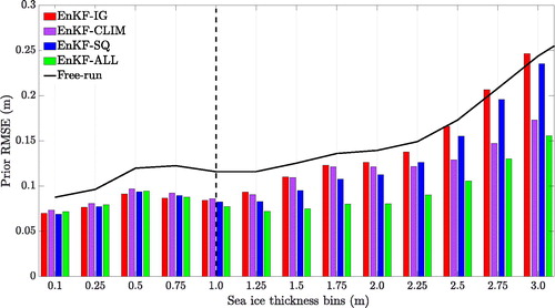
Figure 8 suggests that RMSE values for all schemes below 1 m of SIT are approximately the same, as they all assimilate hard data. If one excludes the EnKF-ALL which is expected to be the most accurate, the EnKF-SQ performs better in the range from 1 m to 2 m where the assimilation of soft data clearly enhances the accuracy compared to the EnKF-CLIM and EnKF-IG. A different choice of climatology may have led to a different interval of thickness but should still prove the EnKF-SQ advantageous for thicknesses slightly above the threshold whatever the choice of climatology. The performance of the EnKF-SQ is not as good as the EnKF-CLIM for thicker ice, which can also be seen in Fig. 7 around the northern coast of Greenland. It is worth noticing that even though there is no data to assimilate for SIT > 1 m in the EnKF-IG scheme, it is performing better than the Free-run up to 2.25 m of SIT. This advantage has been previously reported by Xie et al. (2016, see Fig. 8) and can be either due to the reduction of the positive bias in the free run (shown in Fig. 9) by assimilating thin ice only or due to dynamical model adjustments after assimilation. In other words, improvements to thin ice are propagated in time to the period where ice gets thicker.

Fig. 9. Bar chart of time-averaged posterior bias for SIT obtained from all tested DA schemes. Solid black line represents the time-averaged bias for SIT obtained using the Free-run. Red dotted line represents the time-averaged difference of climatology and truth. SIT bins are displayed on the x-axis with a bin size of 25 cm. Reported in the legend are the time-averaged-weighted total mean bias including the bins for ice thicker than 3 m, which is not shown here. The weights are computed as a fraction of the number of grid cells falling in specific bin interval over total number of grid cells.

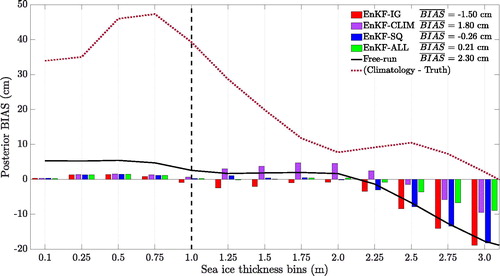
4.3. Bias and skewness analysis

The EnKF-IG updates the prior members by only assimilating observations of thin ice with a maximum thickness of 1 m. This causes the algorithm to introduce negative conditional bias for thick ice (knowing that the observation is thin ice, the assimilation reduces the ice thickness more than that it can thicken it). Similarly, the EnKF-SQ update may introduce a bias towards the detection limit due to assimilation of soft data and the EnKF-CLIM towards the climatology. To investigate these likely biases in different DA schemes, we present a bar chart of time-averaged conditional bias for the posterior estimates of SIT in Fig. 9. The conditional bias is calculated by finding the location of the grid cells for which the observations fall within the SIT bin interval. The positive values represent an overestimation of SIT after the assimilation and vice versa.

The four DA runs exhibit a small negligible positive bias of approximately 0.5 to 1 cm for thin ice. The Free-run bias, on the other hand, is larger than $\sim 6$ cm. Above the threshold limit, there is a clear positive bias of 5 to 7 cm in the EnKF-CLIM posterior estimates, up until 2 m. As seen earlier, the climatology tends to overestimate the truth during the first few months of the experiment when the ice is thin (red dotted line in Fig. 9). EnKF-IG estimates, over the same interval, exhibit a small negative bias, possibly left over from the conditional assimilation of thin ice. It is important to note that there is almost zero bias in the EnKF-SQ estimates, matching that of the EnKF-ALL for $1\le \text{SIT}\le 2$ m. The magnitude by which the climatology is overestimating the truth may vary depending on the choice how one construct it, but nonetheless EnKF-SQ should still produce bias-free estimates in the vicinity of the threshold limit.

There is a systematic increasing negative bias for SIT > 2 m, which reaches almost 20 cm for SIT $=3$ m in the Free-run, EnKF-IG and EnKF-SQ. A similar trend of negative bias is also observed in the EnKF-ALL and EnKF-CLIM runs but to a slightly lesser extent. The negative bias in the Free-Run is likely due to the perturbation of the forcing fields, specifically the wind perturbations, which can cause erratic movements of ice that export thicker sea ice into areas of thinner ice. Since all assimilation runs use perturbed winds, this effect is likely to impact the EnKF-IG and EnKF-SQ more than the EnKF-ALL and EnKF-CLIM. In addition, it is important to mention that there are fewer grid points (not shown here) in the bins for thicker ice compared to thin ice, which may also affect the estimation of the bias for these bins, making them statistically less significant.

As discussed in Shah et al. (2018), the two-piece Gaussian observation likelihood may influence the shape of the posterior distribution, making it skewed and thus less Gaussian. In order to examine this, we evaluate and plot the conditional skewness of the posterior estimates of SIT only at the last assimilation step in Fig. 10. The conditional skewness of the posterior is calculated as the average value of the skewness for all grid cells where the truth falls within the interval of a bin in consideration. Note that contrary to the computation of the conditional BIAS at the location of the observations, the conditional skewness is computed at the truth locations.

Fig. 10. Bar chart of the conditional posterior skewness for SIT estimates obtained using all tested DA schemes and computed at the final assimilation time. Dashed black line represents the detection limit of 1 m SIT.

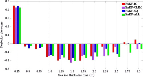
As shown in the figure, thin ice (SIT $\le 25$ cm) yields noticeable skewness in the posterior estimates for all schemes. In the first bin, the truth is close to zero meters (open water) and hence all instances where thin ice has melted in the assimilation run count as zero value. On the other hand, freezing instances lead to various thickness values above 25 cm. Both effect together can make the distribution skewed. The bin between zero and 10 cm shows even larger skewness and has been removed for a better visual presentation. Other than the first bin, a small negative skewness is observed for all the schemes. One possible explanation is the fast melting of ice, drifting over warm waters; a situation enhanced by the lack of coupling with the ocean in the assimilation. This result confirms that the EnKF-SQ, although it uses a skew 2-piece Gaussian likelihood, does not introduce any noticeable positive skewness in its posterior.

4.4. Physical consistency

Ice-ocean models are essential tools for computing integrated quantities that are often difficult to estimate from observations only. Sea ice volume and water transport between ocean basins are such high interest quantities for climate studies. Therefore, it is important to evaluate these quantities to verify that the use of data assimilation does not cause physical inconsistencies.

The total sea ice volume is the integral of sea ice concentration times the sea ice thickness over the entire model area. Its evolution for the different assimilation runs is shown in Fig. 11a. The difference between the assimilation runs compared to the true sea ice volume (Fig. 11b) is relatively small. This is because none of the DA schemes has extensively added or removed ice during the assimilation run. In Fig. 11b a classical seesaw Kalman update behavior is observed. The comparison also reveals that most methods tend to underestimate the ice volume except for EnKF-CLIM.

Fig. 11. (a) Daily ensemble average of sea ice volume over the TOPAZ4 model area for the entire experiment time. (b) Difference of sea ice volume from the truth and all tested DA schemes.

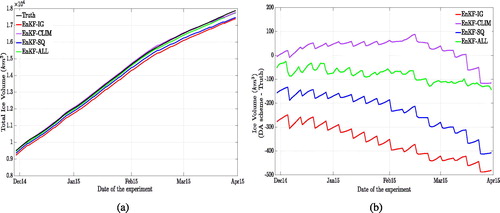
As described earlier, the EnKF-IG has a negative SIT bias, which translates to a nominal loss of between 300 km³ to 500 km³ of sea ice volume from the beginning to the end of the winter (less than 3% of the total simulated ice volume). Seesaw of the time series curves confirm that the EnKF-IG update does remove some ice, which grows back during the subsequent TOPAZ4 model run. The EnKF-SQ does only partially mitigate this loss by 100 to 200 km³ of ice. Surprisingly, the EnKF-ALL is not bias-free either with a loss of up to 100 km³ of ice, which can be caused by various sub-optimal aspects of the data assimilation system, in particular the aforementioned effect of wind perturbations on the areas of thickest ice and the weakly coupled DA. These effects also contribute to the low bias in the other two methods.

The EnKF-CLIM ice volume is closest to the truth run with a little overestimation in the beginning of the winter, then an underestimation in the spring. The construction of the climatological data can explain this trend: since SIT data above one meter only have been retained, the climatology overestimates the SIT in the beginning of the winter but then underestimates the SIT in the midst of the winter because it also accounts for summer SIT. A different construction of the SIT climatology data would have led to a different tendency in EnKF-CLIM.

5. Discussion and conclusions

The purpose of this paper is to demonstrate the usefulness of assimilating range-limited observations with the new EnKF-SQ DA scheme under a realistic experimental setup. Compared to the stochastic EnKF, the main algorithmic difference is the need to compute a different Kalman gain for each ensemble member, depending on the location of the member to the threshold when the observation is out-of-range. This does not make the EnKF-SQ less efficient, but rather prevents the algorithm from being included as a simple extension of existing EnKF codes: it cannot be expressed with an ensemble transform matrix.

Different assimilation experiments are conducted to assess the performance of the EnKF-SQ against other EnKF configurations assimilating only thin ice; both thin and thick ice; and climatology during a winter period in the Arctic. The study shows that assimilating soft data improves the forecast accuracy compared to ignoring them by approximately 8%, particularly where sea ice approaches the detection limit. Such a difference can be important in the performance of an operational system.

The performance exhibited by assimilating a reasonably accurate climatology was similar to the EnKF-SQ. Also, our choice of climatology being annual rather than seasonal may explain some of the flaws in the EnKF-CLIM. Nonetheless, the context of twin experiments is very favorable to EnKF-CLIM because the climatological truth is accurately known; a case which is not true in realistic situations. For instance, in summer there are very few ice thickness measurements and thus it is difficult to construct a meaningful climatology. To this end, it is essential to investigate and compare the performance of the EnKF-SQ and EnKF-CLIM in a context of a biased model twin experiment and with a range of toy models (from linear to non linear regimes).

Assessing the bias of the analysis showed that there is no introduction of any significant bias by the EnKF-SQ, other than the negative bias for thicker ice which is observed in all tested DA schemes. Likewise, the posterior distributions resulting from the application of the EnKF-SQ did not consist of any noticeable higher order moments that could result in undesirable non-Gaussian features because of the two-piece Gaussian likelihood. This is most likely the case for all realistic applications where one would expect relatively small assimilation updates coming regularly in time. The conditional statistics introduced in this paper represent new assessment metrics which were not used in Shah et al. (2018).

As noted in the introduction, the fixed detection limit of 1 m is a convenient simplification in the present twin experiment and should in practice depend on the state of deformation of the ice. The sensitivity experiments in Shah et al. (2018) indicate however that the present findings should still hold with different values of the detection limit for SIT. Furthermore, the choice of out-of-range (OR) observation error variance was not found to be very critical. A wide range of values for this parameter were tested and lead to acceptable performance of the EnKF-SQ. Ways of estimating ${\sigma }_{or}^2$ adaptively in space and time is currently being investigated and will be reported in a follow-up study. Concerning the physical constraints of the model, the EnKF-SQ estimates were found to be physically consistent and comparable to other tested assimilation schemes.

The assimilation of synthetic sea ice thickness data with a upper detection limit of 1 m in a coupled ice-ocean model of TOPAZ4 is demonstrated using the EnKF-SQ and shown to have a useful impact on SIT estimates. The results obtained with SMOS-like observations can be generalised to CryoSat2-like observations by reversing the upper limit into a lower limit. Thus, merging the two products may not be necessary because each satellite data can be assimilated in a separate EnKF-SQ step. The EnKF-SQ therefore makes a viable data assimilation strategy for range-limited observations in high-dimensional nonlinear systems. Future research will focus on assimilating real data, in which the EnKF-SQ is confronted with large observation biases unlike the presented twin experiments setup.

Disclosure statement

No potential conflict of interest was reported by the authors.

Additional information

Funding

The research is funded by the Nordic Center of Excellence EmblA (Ensemble-based data assimilation for environmental monitoring and prediction) under NordForsk contract number 56801. The Copernicus Marine Services and the Nansen Scientific Society have also contributed to the funding. Norwegian grants of the computer time (nn2993k) and data storage space (ns2993k) have also been used for the simulations. The salary for François Counillon was co-funded by the NordForsk under the Nordic Center of Excellence (ARCPATH, 76654), and the Trond Mohn Foundation under the project number BFS2018TMT01.

Notes

1 It should be noted that the comparison of assimilating merged versus separate data is not informative because their observation errors are not equivalent.

2 σ_ir is a special case of σ_h, for hard data at the detection limit.

References

- Aagaard, K. and Carmack, E. C. 1989. The role of sea ice and other fresh water in the Arctic circulation. J. Geophys. Res. 94, 14485–14498. doi:10.1029/JC094iC10p14485
- Bentsen, M., Evensen, G., Drange, H. and Jenkins, A. D. 1999. Coordinate transformation on a sphere using conformal mapping. Mon. Weather Rev. 127, 2733–2740. doi:10.1175/1520-0493(1999)127<2733:CTOASU>2.0.CO;2
- Bleck, R. 2002. An oceanic general circulation model framed in hybrid isopycnic-cartesian coordinates. Ocean Model. 4, 55–88. doi:10.1016/S1463-5003(01)00012-9
- Borup, M., Grum, M., Madsen, H. and Mikkelsen, P. S. 2015. A partial ensemble Kalman filtering approach to enable use of range limited observations. Stoch. Environ. Res. Risk Assess. 29, 119–129. Online at: doi:10.1007/s00477-014-0908-1
- Bouillon, S., Fichefet, T., Legat, V. and Madec, G. 2013. The elastic–viscous–plastic method revisited. Ocean Model. 71, 2–12. Part of special issue: Arctic Ocean. doi:10.1016/j.ocemod.2013.05.013
- Burgers, G., Jan van Leeuwen, P. and Evensen, G. 1998. Analysis scheme in the ensemble Kalman filter. Mon. Weather Rev. 126, 1719–1724. doi:10.1175/1520-0493(1998)126<1719:ASITEK>2.0.CO;2
- Chassignet, E. P., Smith, L. T., Halliwell, G. R. and Bleck, R. 2003. North Atlantic simulations with the hybrid coordinate ocean model (HYCOM): Impact of the vertical coordinate choice, reference pressure, and thermobaricity. J. Phys. Oceanogr. 33, 2504–2526. doi:10.1175/1520-0485(2003)033<2504:NASWTH>2.0.CO;2
- Collow, T. W., Wang, W., Kumar, A. and Zhang, J. 2015. Improving Arctic sea ice prediction using PIOMAS initial sea ice thickness in a coupled ocean-atmosphere model. Mon. Weather Rev. 143, 4618–4630. doi:10.1175/MWR-D-15-0097.1
- Connor, L. N., Laxon, S. W., Ridout, A. L., Krabill, W. B. and McAdoo, D. C. 2009. Comparison of Envisat radar and airborne laser altimeter measurements over Arctic sea ice. Remote Sens. Environ. 113, 563–570. doi:10.1016/j.rse.2008.10.015
- Day, J. J., Hawkins, E. and Tietsche, S. 2014. Will Arctic sea ice thickness initialization improve seasonal forecast skill? Geophys. Res. Lett. 41, 7566–7575. doi:10.1002/2014GL061694
- Dee, D. P., Uppala, S. M., Simmons, A. J., Berrisford, P., Poli, P. and co-authors. 2011. The ERA-Interim reanalysis: Configuration and performance of the data assimilation system. Q. J. R. Meteorol. Soc. 137, 553–597. doi:10.1002/qj.828
- Drange, H. and Simonsen, K. 1996. Formulation of Air-Sea Fluxes in the ESOP2 Version of MICOM. Technical Report 125, Nansen Environmental and Remote Sensing Center, Bergen.
- Evensen, G. 2003. The ensemble Kalman filter: Theoretical formulation and practical implementation. Ocean Dyn. 53, 343–367. doi:10.1007/s10236-003-0036-9
- Evensen, G. 2004. Sampling strategies and square root analysis schemes for the EnKF. Ocean Dyn. 54, 539–560. doi:10.1007/s10236-004-0099-2
- Forsberg, R. and Skourup, H. 2005. Arctic Ocean gravity, geoid and sea-ice freeboard heights from ICESat and GRACE. Geophys. Res. Lett. 32, L21502. doi:10.1029/2005GL023711
- Fritzner, S., Graversen, R., Christensen, K. H., Rostosky, P. and Wang, K. 2019. Impact of assimilating sea ice concentration, sea ice thickness and snow depth in a coupled ocean-sea ice modelling system. Cryosphere 13, 491–509. doi:10.5194/tc-13-491-2019
- Guemas, V., Blanchard-Wrigglesworth, E., Chevallier, M., Day, J. J., Déqué, M. and co-authors. 2016. A review on Arctic sea-ice predictability and prediction on seasonal to decadal time-scales. Q. J. R. Meteorol. Soc. 142, 546–561. doi:10.1002/qj.2401
- Houtekamer, P. L. and Mitchell, H. L. 1998. Data assimilation using an ensemble Kalman filter technique. Mon. Weather Rev. 126, 796–811. doi:10.1175/1520-0493(1998)126<0796:DAUAEK>2.0.CO;2
- Hunke, E. C. and Dukowicz, J. K. 1997. An elastic–viscous–plastic model for sea ice dynamics. J. Phys. Oceanogr. 27, 1849–1867. doi:10.1175/1520-0485(1997)027<1849:AEVPMF>2.0.CO;2
- Huntemann, M., Heygster, G., Kaleschke, L., Krumpen, T., Mäkynen, M. and co-authors. 2014. Empirical sea ice thickness retrieval during the freeze-up period from SMOS high incident angle observations. Cryosphere 8, 439–451. doi:10.5194/tc-8-439-2014
- Kaleschke, L., Maaß, N., Haas, C., Hendricks, S., Heygster, G. and co-authors. 2010. A sea-ice thickness retrieval model for 1.4 GHz radiometry and application to airborne measurements over low salinity sea-ice. Cryosphere 4, 583–592. doi:10.5194/tc-4-583-2010
- Kaleschke, L., Tian-Kunze, X., Maas, N., Ricker, R., Hendricks, S. and Drusch, M.2015. Improved retrieval of sea ice thickness from SMOS and CryoSat-2. 2015 IEEE International Geoscience and Remote Sensing Symposium (IGARSS), Milan, 2015, pp 5232–5235. doi:10.1109/IGARSS.2015.7327014
- Kimmritz, M., Counillon, F., Bitz, C., Massonnet, F., Bethke, I. and co-authors. 2018. Optimising assimilation of sea ice concentration in an Earth system model with a multicategory sea ice model. Tellus A: Dynamic Meteorology and Oceanography 70, 1–23. doi:10.1080/16000870.2018.1435945
- Laxon, S. W., Giles, K. A., Ridout, A. L., Wingham, D. J., Willatt, R. and co-authors. 2013. CryoSat-2 estimates of Arctic sea ice thickness and volume. Geophys. Res. Lett. 40, 732–737. doi:10.1002/grl.50193
- Mu, L., Losch, M., Yang, Q., Ricker, R., Losa, S. N. and co-authors. 2018. Arctic-wide sea ice thickness estimates from combining satellite remote sensing data and a dynamic ice-ocean model with data assimilation during the CryoSat-2 period. J. Geophys. Res. Oceans 123, 7763–7780. doi:10.1029/2018JC014316
- Ricker, R., Hendricks, S., Helm, V., Skourup, H. and Davidson, M. 2014. Sensitivity of CryoSat-2 Arctic sea-ice freeboard and thickness on radar-waveform interpretation. The Cryosphere 8, 1607–1622. doi:10.5194/tc-8-1607-2014
- Ricker, R., Hendricks, S., Kaleschke, L., Tian-Kunze, X., King, J. and co-authors. 2017. A weekly Arctic sea-ice thickness data record from merged CryoSat-2 and SMOS satellite data. The Cryosphere 11, 1607–1623. doi:10.5194/tc-11-1607-2017
- Sakov, P., Counillon, F., Bertino, L., Lisaeter, K., Oke, P. and co-authors. 2012. TOPAZ4: An ocean-sea ice data assimilation system for the north Atlantic and Arctic. Ocean Sci. 8, 633. doi:10.5194/os-8-633-2012
- Screen, J. and Simmonds, I. 2010. The central role of diminishing sea ice in recent Arctic temperature amplification. Nature 464, 1334–1337. doi:10.1038/nature09051
- Shah, A., Gharamti, M. E. and Bertino, L. 2018. Assimilation of semi-qualitative observations with a stochastic ensemble kalman filter. Q. J. R. Meteorol. Soc.144, 1882–1894. doi:10.1002/qj.3381
- Tian-Kunze, X., Kaleschke, L., Maaß, N., Mäkynen, M., Serra, N. and co-authors. 2014. SMOS-derived thin sea ice thickness: Algorithm baseline, product specifications and initial verification. Cryosphere 8, 997–1018. doi:10.5194/tc-8-997-2014
- Tilling, R. L., Ridout, A. and Shepherd, A. 2016. Near-real-time Arctic sea ice thickness and volume from CryoSat-2. Cryosphere 10, 2003–2012. doi:10.5194/tc-10-2003-2016
- Wang, X., Key, J., Kwok, R. and Zhang, J. 2016. Comparison of Arctic sea ice thickness from satellites, aircraft, and PIOMAS data. Remote Sens. 8, 713. doi:10.3390/rs8090713
- Xie, J., Bertino, L., Counillon, F., Lisaeter, K. A. and Sakov, P. 2017. Quality assessment of the TOPAZ4 reanalysis in the Arctic over the period 1991–2013. Ocean Sci. 13, 123–144. doi:10.5194/os-13-123-2017
- Xie, J., Counillon, F. and Bertino, L. 2018. Impact of assimilating a merged sea-ice thickness from cryosat-2 and smos in the arctic reanalysis. Cryosphere 12, 3671–3691. doi:10.5194/tc-12-3671-2018
- Xie, J., Counillon, F., Bertino, L., Tian-Kunze, X. and Kaleschke, L. 2016. Benefits of assimilating thin sea ice thickness from SMOS into the TOPAZ system. Cryosphere 10, 2745–2761. doi:10.5194/tc-10-2745-2016
- Yang, Q., Losa, S. N., Losch, M., Tian-Kunze, X., Nerger, L. and co-authors. 2014. Assimilating SMOS sea ice thickness into a coupled ice-ocean model using a local SEIK filter. J. Geophys. Res. Oceans 119, 6680–6692. doi:10.1002/2014JC009963