Application of observability Gramian to targeted observation in WRF data assimilation

Abstract

The optimal observation placement in weather forecast and research (WRF) data assimilation is investigated using a sensitivity analysis method. The method quantifies the sensitivity of observation location to assimilated results as an unobservability index. The empirical observability Gramian matrix composed from a time series of WRF model outputs is used to obtain the unobservability index in the WRF domain. A three-dimensional variational data assimilation (3 D-VAR) method is employed in the WRF model to assimilate the observations of horizontal winds, whose locations are selected based on the unobservability index. The results from the identical-twin experiments show a correlation between improvement in the assimilated wind field and the magnitude of unobservability index. The temporal variation of the vertical component of vorticity is strongly related to the unobservability index, which confirms that an observation location exhibiting a high unobservability index contributes to error reduction in the data assimilation owing to the reduction in the uncertainty caused by the strong vorticity changes.

Keywords:

• targeted observation
• weather forecasting
• observability
• data assimilation
• WRF

1. Introduction

Wind farms are recognised as one of the most promising reusable energy sources (REN21, 2018). The worldwide trend of using renewable energy results in global market expansion, and the growing number of wind farms increases the demand for accurate prediction of atmospheric wind states. Electric power generated by a wind farm tends to be unstable because of changes in weather conditions, which cannot be avoided in the atmospheric system. It is also known that the short-term prediction of wind power generation is not sufficiently accurate to control a wind farm, as reported by Enomoto (2006), showing the limitations of the statistical sustainable model in short-term wind prediction.

The sensitivity of numerical weather prediction (NWP) to initial conditions originates from the chaotic behaviour of an atmospheric model (Lorenz, 1963). Numerical models have uncertainties; thus, long-term integration could produce a significantly different result. Accurate wind prediction is mandatory for estimating the amount of generated power because it strongly depends on changes in the wind state. In such a situation, it is expected that data assimilation would improve numerical weather forecasts by decreasing the uncertainties in the initial values with the help of observations in the real world.

Concerning data assimilation in a limited area, such as a wind farm, it is important to know which observation location is optimal for data assimilation, because there are many methods to be used for observations depending on the locations, such as an anemometer, a wind profiler, a radiosonde, and light detection and ranging (LIDAR). The optimisation of observation locations to improve the NWP is known as targeted observations. Several methods have been proposed to conduct targeted observations. Baker and Daley (2000) and Langland and Baker (2004) proposed adjoint-based methods to assess the observation impact. Liu and Kalnay (2008), Liu et al. (2009), and Li et al. (2009) proposed a method using an ensemble prediction, which has similar capability as the adjoint method with less effort to handle an adjoint code. As for the sensitivity analysis method, Buizza et al. (2007b), Cardinali et al. (2007), and Kelly et al. (2007) showed that observations based on the singular vector-based sensitivity of the Pacific and Atlantic Oceans have more advantages than observations in other regions. Carrassi et al. (2007) carried out Observing System Simulation Experiments (OSSEs) in a quasi-geostrophic (QG) model and ensured the effect of an adaptive observation method using the bred vectors proposed by Toth and Kalnay (1993), which effectively capture the characteristic error growth modes of a field.

Kang and Xu (2009) proposed an approach for sensitivity analysis, originated from modern control theory, to estimate the preferable observation locations for data assimilation. Compared with the concept of observation sensitivity, which is a typical method in targeted observations, this proposed method uses the observation model but not the data from observations; the information of the optimal observation configuration can be found before the assimilation is performed. In modern control theory, the system’s observability can be assessed by the regularity of the observability Gramian. However, the condition does not provide the degree of observability in a quantitative sense; moreover, it is difficult to compose the Gramian explicitly from high-dimensional models. In large models, the effectiveness of observation locations can be quantified by an eigenvalue of the empirical observability Gramian constructed from the results of a numerical model. When the observability for a set of points is quantified, an observation configuration with a higher observability contains more information with which to understand the internal states of the system and is more effective in eliciting a future state prediction. It is also beneficial that the approach is independent of any data assimilation method; as such, it can be combined with many types of methods, such as 4 D-VAR, ensemble Kalman filter, and particle filter. The effectiveness of this approach was demonstrated using simple mathematical models in Kang and Xu (2012) and King et al. (2013). Recently, there have been practical achievements of the empirical observability Gramian in the optimal placement of the phasor measurement units (PMUs) used in electric power systems (Qi et al., 2015, 2016). As mentioned above, several methods have been proposed to evaluate the impact of observation; however, there have not been examples of the observability used in targeted observations for weather forecasting. Therefore, there is still a room for clarifying the relation between the observability and a wind field considered in an NWP model.

In this study, the method formulated by Kang and Xu (2009) is applied to a data assimilation problem in weather forecasting with the Weather Research and Forecast-Advanced Research WRF (WRF-ARW) Version 3.8 (Skamarock et al., 2008) model. Although our final target is the optimisation of observation locations in a wind farm, the applicability of this method is investigated in meso-scale weather forecasting covering the eastern Japan as a preliminary assessment. First, the observability estimated by the empirical observability Gramian is studied in detail by comparing with the corresponding wind field in an identical-twin experiment. For this experiment, three-dimensional variational data assimilation (3 D-VAR) (Barker et al., 2003) from WRF Data Assimilation (WRFDA) Version 3.8 (Barker et al., 2003, 2012) software is employed. Compared to other data assimilation methods, 3 D-VAR has advantages in numerical costs, which is important for short-term wind prediction in wind farm applications.

This paper is organised as follows. The computational methods are presented in Section 2. The relation between the observability and corresponding wind field is detailed in Section 3.1. The identical-twin experiment for wind-state forecasting is discussed using the eigenvalues of an empirical observability Gramian in Section 3.2. Finally, we conclude this study in Section 4.

2. Computational methods

2.1. Evaluation of observability

In this study, sensitivity analysis is conducted using the method proposed by Kang and Xu (2009), which is based on the observability in modern control theory. The definition of the observability is presented in this section. The unobservability index$\mathrm{}\rho /ϵ$ (Krener and Ide, 2009) quantifies the observability of a system. According to Kang and Xu (2009), the parameters$\mathrm{}\rho \mathrm{}(>0)$ and$\mathrm{}\mathrm{ϵ}$ are defined as: (1) $${\mathrm{ϵ}}^2=\underset{\delta x_0}{\min }L\left({\mathit{x}}_0,\delta {\mathit{x}}_0,\lambda \right)\mathrm{}\mathit{subject}\mathrm{}to\mathrm{}\left|\delta {\mathit{x}}_0\right|=\rho ,$$(1) where $L\left({\mathit{x}}_0,\delta {\mathit{x}}_0,\lambda \right)$ is a function defined as: (2) $$L\left({\mathit{x}}_0,\delta {\mathit{x}}_0,\lambda \right)=\sum _{k=1}^N{\left(\mathit{y}\left(t_k,{\mathit{x}}_0+\delta {\mathit{x}}_0,\lambda \right)-{\mathit{y}}_k\left({\mathit{x}}_0,\lambda \right)\right)}^T{\mathit{R}}_k\left(\mathit{y}\left(t_k,{\mathit{x}}_0+\delta {\mathit{x}}_0,\lambda \right)-{\mathit{y}}_k\left({\mathit{x}}_0,\lambda \right)\right)=\sum _{k=1}^N{\left|\mathit{y}\left({t_k,\mathit{x}}_0+\delta {\mathit{x}}_0,\lambda \right)-\mathit{y}\left({t_k,\mathit{x}}_0,\lambda \right)\right|}_{{\mathit{R}}_k}^2.$$(2)

Here, ${\mathit{x}}_0$ and $\mathit{y}\left(t_k,{\mathit{x}}_0,\lambda \right)$ are the initial value of the system and the observations sampled at observation location $\lambda$ in a model trajectory starting from ${\mathit{x}}_0.$ In this study, ${\mathit{R}}_k$ is set to an identity matrix, which assumes no correlation between different observations. Parameter $ϵ$ is the minimum value of L subject to the constraint of initial disturbance $\mathrm{\delta }{\mathit{x}}_0\mathrm{}$ whose norm is positive constant$\mathrm{}\rho .$ In addition, N indicates the number of time steps for the WRF model run. If the system is linear $({\mathit{x}}_{k+1}=\mathit{A}{\mathit{x}}_k,\mathrm{}{\mathit{y}}_k={\mathit{C}}_{\lambda }{\mathit{x}}_k),$ $\mathrm{ϵ}$ is calculated using the minimum eigenvalue of the observability Gramian ${\mathit{W}}_o$ and $\rho$ as follows: (3) $${\mathrm{ϵ}}^2=\underset{\delta x_0}{\min }L\left({\mathit{x}}_0,\delta {\mathit{x}}_0,\lambda \right)$$(3) $$=\underset{\delta x_0}{\min }\sum _{k=1}^N{\left|\mathit{y}\left({t_k,\mathit{x}}_0+\delta {\mathit{x}}_0,\lambda \right)-\mathit{y}\left({t_k,\mathit{x}}_0,\lambda \right)\right|}_{R_i}^2$$ $$=\underset{\delta x_0}{\min }\delta {\mathit{x}}_0^{\mathit{T}}\left(\sum _{k=1}^N{{\left({\mathit{A}}^k\right)}^T{\mathit{C}}_{\lambda }^T\mathit{C}}_{\lambda }{\mathit{A}}^k\right)\delta {\mathit{x}}_0$$ $$=\underset{\delta x_0}{\min }\delta {\mathit{x}}_0^{\mathit{T}}{\mathit{W}}_{\mathrm{o}}\delta {\mathit{x}}_0$$ (4) $$={\sigma }_{\mathit{min}}{\rho }^2.$$(4)

Using Equations (3)(3) $${\mathrm{ϵ}}^2=\underset{\delta x_0}{\min }L\left({\mathit{x}}_0,\delta {\mathit{x}}_0,\lambda \right)$$(3) and (4)(4) $$={\sigma }_{\mathit{min}}{\rho }^2.$$(4) , the unobservability index can be calculated as: (5) $$\frac{\rho }{ϵ}=\frac{1}{\sqrt{{\sigma }_{\mathit{min}}}}.$$(5)

In this study, the observability is evaluated with ${\sigma }_{\mathit{min}}$ because the unobservability index and square root of the minimum eigenvalue $\sqrt{{\sigma }_{\mathit{min}}}$ are inversely proportional as in Equation (5)(5) $$\frac{\rho }{ϵ}=\frac{1}{\sqrt{{\sigma }_{\mathit{min}}}}.$$(5) . A smaller unobservability index, i.e. a larger minimum eigenvalue results in a larger observability.

2.2. Empirical observability Gramian

The calculation of an observability Gramian ${\mathit{W}}_{\mathrm{o}}$ for very large systems, such as NWP, is extremely expensive; thus, a method that empirically composes an observability Gramian from model outputs is employed following the approach of Krener and Ide (2009) and Kang and Xu (2009). In this approach, the observability of wind magnitude $\sqrt{u^2+v^2}$ is estimated using an observation matrix and several trajectories of $u$ (wind x-component) and $v$ (wind y-component) from the disturbed initial wind fields calculated by the WRF model.

The empirical observability Gramian $\mathit{G}$ is obtained by: (6) $$\mathit{G}=\sum _{k=1}^N{\mathit{Y}}_k^T{{\mathit{R}}_k\mathit{Y}}_k,$$(6) with a matrix ${\mathit{Y}}_k:$ (7) $${\mathit{Y}}_k=\left[\begin{array}{cc}\Delta y_{k,1,\lambda }& \Delta y_{k,2,\lambda }\end{array}\mathrm{}\begin{array}{cc}\cdots & \Delta y_{k,r,\lambda }\end{array}\right],$$(7) where each vector element is calculated as: (8) $$\Delta y_{k,j,\lambda }=\frac{1}{2\rho }\left[\mathit{y}\left({t_k,\mathit{x}}_0+\rho \delta {\mathit{x}}_{0,j},\lambda \right)-\mathit{y}\left({t_k,\mathit{x}}_0-\rho \delta {\mathit{x}}_{0,j},\lambda \right)\right].$$(8)

The vector $\Delta y_{k,j,\lambda }$ is obtained by the difference in the observed states at a set of locations $\lambda$ between trajectories from different initial values, ${\mathit{x}}_0+\rho \mathit{\delta }{\mathit{x}}_{0,j}$ and ${\mathit{x}}_0-\rho {\mathit{\delta }\mathit{x}}_{0,j}$ at a particular sampling time k. In Equation (8)(8) $$\Delta y_{k,j,\lambda }=\frac{1}{2\rho }\left[\mathit{y}\left({t_k,\mathit{x}}_0+\rho \delta {\mathit{x}}_{0,j},\lambda \right)-\mathit{y}\left({t_k,\mathit{x}}_0-\rho \delta {\mathit{x}}_{0,j},\lambda \right)\right].$$(8) , $\rho$ determines the size of perturbation $\delta {\mathit{x}}_{0,j},$ while r sets of initial perturbations $\delta {\mathit{x}}_{0,j}$ ($1\le j\le r$) are considered. Thus, the required number of WRF model runs is 2r times with initial conditions perturbed by $\pm \rho \mathit{\delta }{\mathit{x}}_{0,j}.$ The initial disturbance is defined by spatial modes from proper orthogonal decomposition (POD), which will be described in the following section.

2.3. Snapshot POD

POD, also known as principal component analysis (PCA), or empirical orthogonal function (EOF), can be used to decompose the spatiotemporal variation of a field into orthogonal bases (POD bases or POD modes, hereafter) which optimally represent the variation. In this study, the POD modes obtained from the WRF model run are used as initial disturbance $\delta {\mathit{x}}_{0,j}$ in Equation (8)(8) $$\Delta y_{k,j,\lambda }=\frac{1}{2\rho }\left[\mathit{y}\left({t_k,\mathit{x}}_0+\rho \delta {\mathit{x}}_{0,j},\lambda \right)-\mathit{y}\left({t_k,\mathit{x}}_0-\rho \delta {\mathit{x}}_{0,j},\lambda \right)\right].$$(8) . Particularly, the snapshot POD (Sirovich, 1987) is used to generate POD bases from WRF model outputs with a certain sampling interval. It is extremely expensive to obtain POD modes directly because the outputs from large models, such as NWP, normally have a dimension of n (∼10⁷) that is too large to solve an eigenvalue problem. The snapshot POD procedure reduces the size of the problem on the order of m (∼10², ∼ the number of snapshots) and calculates the eigenvalue problem for an m × m matrix to obtain POD modes.

These POD modes are expected to be effective as an initial perturbation to calculate the empirical observability Gramian in Section 2.2, because they show representative spatiotemporal variations of a wind field during a time period of interest. Matrix $\mathit{X}$ can be composed of column vectors of horizontal wind components $\mathit{u}$ and $\mathit{v}$ from a WRF model run with a certain time interval as: (9) $$\mathit{X}=\left[\begin{array}{ccc}{\mathit{u}}_1& \cdots & {\mathit{u}}_m\\ {\mathit{v}}_1& \cdots & {\mathit{v}}_m\end{array}\right],$$(9) where m indicates the number of snapshots. The matrix ${\mathit{X}}^T\mathit{X}$ can be decomposed by using a singular value decomposition (SVD) algorithm as: (10) $${\mathit{X}}^T\mathit{X}=\mathit{V}{\mathit{S}}^2{\mathit{V}}^T\left(=\mathit{VS}{\mathit{U}}^T\mathit{U}\mathit{S}{\mathit{V}}^T\right),$$(10) where $\mathit{V}$ is the eigenvector and ${\mathit{S}}^2$ corresponds to the eigenvalue. The POD modes $\mathit{U}$ can be represented by: (11) $$\mathit{U}=\mathit{XV}{\mathit{S}}^{-1}.$$(11)

The resulting POD modes $\mathit{U}=[\delta {\mathit{x}}_{0,1},\mathrm{}\dots ,\mathrm{}\delta {\mathit{x}}_{0,m}]$ are used as initial perturbations to evaluate the empirical observability Gramian. Note that not all the POD modes are used for the empirical observability Gramian. Instead, the leading r modes determined by the cumulative energy ratio are used as the initial perturbation.

2.4. 3 D-var

In this study, 3 D-VAR in WRFDA Version 3.8 is utilised (Barker et al., 2003) as a data assimilation method based on variational analysis, which explores the analysis $\mathit{x}$ that minimises the cost function $J$ as: (13) $$J=J_b\left(\mathit{x}\right)+J_o\left(\mathit{x}\right)=\frac{1}{2}{\left(\mathit{x}-{\mathit{x}}_b\right)}^T{\mathit{B}}^{-1}\left(\mathit{x}-{\mathit{x}}_b\right)+\frac{1}{2}{\left(\mathit{Hx}-{\mathit{y}}_0\right)}^T{(\mathit{E}+\mathit{F})}^{-1}\left(\mathit{Hx}-{\mathit{y}}_0\right),$$(13) where ${\mathit{x}}_b$ is the first-guess of the state and ${\mathit{y}}_0$ is the observation of the state available at that time. The 3 D-VAR routine requires the background error covariance matrix $\mathit{B}$ in advance; thus, $\mathit{B}$ was approximated on the basis of the NMC method (Parrish and Derber, 1992) using the 1-year-averaged 24-h forecast error of GFS with the T170 spatial resolution (Wang et al., 2017). For the observation errors $\mathit{E},$ the wind speed and direction are assumed to have small error of 0.1 m/s and 0.1°, respectively. $\mathit{F}$ is the representativity error covariance matrix of observation matrix $\mathit{H},$ which is given in WRFDA. The cost function in Equation (13)(13) $$J=J_b\left(\mathit{x}\right)+J_o\left(\mathit{x}\right)=\frac{1}{2}{\left(\mathit{x}-{\mathit{x}}_b\right)}^T{\mathit{B}}^{-1}\left(\mathit{x}-{\mathit{x}}_b\right)+\frac{1}{2}{\left(\mathit{Hx}-{\mathit{y}}_0\right)}^T{(\mathit{E}+\mathit{F})}^{-1}\left(\mathit{Hx}-{\mathit{y}}_0\right),$$(13) is minimised using the gradient obtained by: (14) $$\frac{dJ}{d\mathit{x}}={\mathit{B}}^{-1}\left(\mathit{x}-{\mathit{x}}_0\right)+{\mathit{H}}^T{\left(\mathit{E}+\mathit{F}\right)}^{-1}\left(\mathit{Hx}-{\mathit{y}}_0\right).$$(14)

WRFDA decreases the computational cost of 3 D-VAR using a control-variable transform and an incremental method to avoid the direct calculation of B (Barker et al., 2003), which is commonly large. The control-variable transform calculates the analysis increment from the basic variables considered to be independent of each other through the transform matrix ${\mathit{U}}_t.$ The incremental method expresses the cost function with an increment $\mathit{w},$ which is the difference between the analysis and first guess. The transform matrix deforms the cost function, as shown in Equation (15)(15) $$J\left({\mathit{V}}_c\right)=\frac{1}{2}{\mathit{V}}_c^T{\mathit{V}}_c+\frac{1}{2}{\left(\mathit{d}-\mathit{H}{\mathit{U}}_t{\mathit{V}}_c\right)}^T{\mathit{R}}^{-1}\left(\mathit{d}-\mathit{H}{\mathit{U}}_t{\mathit{V}}_c\right).$$(15) , because ${\mathit{U}}_t$ implicitly has the information of the background error: (15) $$J\left({\mathit{V}}_c\right)=\frac{1}{2}{\mathit{V}}_c^T{\mathit{V}}_c+\frac{1}{2}{\left(\mathit{d}-\mathit{H}{\mathit{U}}_t{\mathit{V}}_c\right)}^T{\mathit{R}}^{-1}\left(\mathit{d}-\mathit{H}{\mathit{U}}_t{\mathit{V}}_c\right).$$(15)

Five variables compose the control variables$\mathrm{}{\mathit{V}}_c:$ the stream function, unbalanced velocity potential, unbalanced temperature, pseudo-relative humidity, and unbalanced surface pressure. Equation (16)(16) $${\mathit{U}}_t{\mathit{V}}_c=\mathit{x}-{\mathit{x}}_b=\mathit{w}.$$(16) shows the transform from control variables to model variables: (16) $${\mathit{U}}_t{\mathit{V}}_c=\mathit{x}-{\mathit{x}}_b=\mathit{w}.$$(16)

After this transformation, the increment $\mathit{w}$ is obtained from the model variables.

In WRFDA, it is possible to adjust a background error correlation in $\mathit{B}.$ Correlation $\varphi$ with the shape of the Gaussian distribution is a function of the horizontal distance between two grid points $s$ and spatial length scale $L$ as: (17) $$\varphi \left(s\right)=\exp (-\frac{s^2}{2L}).$$(17)

As will be discussed in subsequent sections, we focus on the atmosphere below the planetary boundary layer; therefore, the spatial length scale is adjusted depending on the altitude levels of interest.

2.5. Evaluation of empirical observability Gramian in WRF

The computational conditions, the domain and a wind field at level 12, are presented in Table 1 and Fig. 1, respectively. In the time period of 2017/2/7 06:00–18:00 GMT, there was a dominant seasonal wind from continental Asia to the Japanese islands caused by a typical pressure pattern of winter in Japan. In addition, small disturbance of the wind field can be seen in the area of the circle A in Fig. 1.

Fig. 1. Computational domain, geographical height, and streamline at the assimilation time (2017/2/7 12:00 GMT) for level 12. The strong northwest wind observed in the figure is caused by a typical pressure pattern of winter in Japan. A small turbulence is found in circle A.

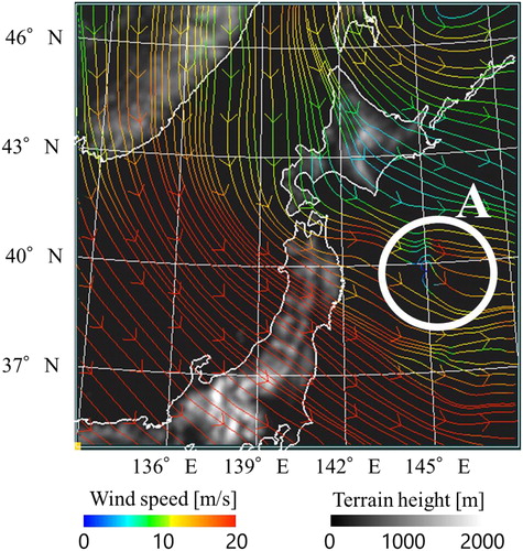
Table 1. Conditions for the observability calculation.

	Computational conditions
Time period (Section 3.1)	2017/2/7 06:00 – 2017/2/7 18:00
Time period (Section 3.2)	2017/2/7 06:00 – 2017/2/7 12:00
Horizontal grid distance	9 km
Number of horizontal grids	151 × 151
Time step interval	15 s
Number of vertical grids	30
Snapshot time interval for POD	15 min
Time interval for measurements	15 min
Number of POD modes used for perturbations	4
Length of time integration	12 h
Variable to be measured	Wind speed [m/s]
Number of measurements	1

The initial condition for the observability analysis is set to the instantaneous field at 2017/2/7 06:00 GMT, and the energy dominant four POD modes (r = 4) are used for the perturbations of the initial wind field. Note that the cumulative energy of those POD modes reaches approximately 99.9%. Using the initial conditions disturbed by the POD modes, time integration is performed for 12-h until 2017/2/7 18:00 GMT, which is 6-h ahead of assimilation. The wind field is acquired every 15 min as a snapshot to construct matrix $\mathit{X},$ which results in 49 snapshots in total. Factor $\rho$ in Equation (8)(8) $$\Delta y_{k,j,\lambda }=\frac{1}{2\rho }\left[\mathit{y}\left({t_k,\mathit{x}}_0+\rho \delta {\mathit{x}}_{0,j},\lambda \right)-\mathit{y}\left({t_k,\mathit{x}}_0-\rho \delta {\mathit{x}}_{0,j},\lambda \right)\right].$$(8) is set to 1000 because each element of the POD bases is on the order of 10⁻⁴ by normalisation during SVD.

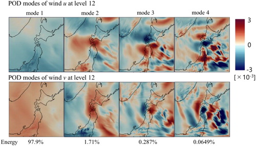
Figure 2 shows the leading four POD modes of wind components $u$ and $v$ that were used for the initial perturbations in level 12.

Fig. 2. Proper orthogonal decomposition (POD) bases for wind components $u$ and $v$ at level 12. Each mode is normalised in whole domain.

2.6. Identical-twin experiment and evaluation

The effectiveness of the empirical observability Gramian on WRF data assimilation is evaluated in an identical-twin experiment. Table 2 summarises the conditions for the identical-twin experiment. $x_{i,\mathrm{}\mathit{true}}$ in Equation (18)(18) $$\text{RMSE}=\sqrt{\frac{1}{N}\sum _{i=1}^N{\left(x_i-x_{i,\mathrm{}\mathit{true}}\right)}^2},$$(18) , the true state, is generated based on the condition in Table 2. JMA-NHM is mainly used to generate initial/boundary conditions for the true state, while NCEP-GFS is used for the first guess.

Table 2. Computational conditions for the identical-twin experiment.

	First guess	True state
Time period	2017/2/7 06:00 – 2017/2/7 18:00	2017/2/6 12:00 – 2017/2/7 18:00
Horizontal grid distance	9 km
Number of horizontal grids	151 × 151
Length of time step	15 s
Number of vertical grids	30
Time for assimilation	2017/2/7 12:00
Observed variable	–	Wind speed [m/s]/Wind direction [°]
Number of Observations for each data assimilation	1
Initial/boundary conditions	NCEP GFS	JMA MSM (NCEP GFS for soil variables)
Time integration scheme	Runge–Kutta 3^rd-order
Cumulus physics	Kain–Fritsch scheme
Surface-layer physics	Revised MM5 Monin–Obukhov scheme
Microphysics	WSM three-class simple ice scheme
PBL scheme	YSU scheme
Radiation scheme	RRTM scheme (Long wave), Dudhia scheme (Short wave)

Data assimilation is performed with one observation every 10 grids horizontally, which means 13 × 13 = 169 assimilations for each level. To evaluate the data assimilation result with/without the targeted observation, the change in the layer-averaged root-mean-square error (RMSE) due to data assimilation is evaluated at each observation point. The RMSE and its change are evaluated by: (18) $$\text{RMSE}=\sqrt{\frac{1}{N}\sum _{i=1}^N{\left(x_i-x_{i,\mathrm{}\mathit{true}}\right)}^2},$$(18) and (19) $$\begin{array}{c}\text{RMSE}\text{change}\\ \text{after}\text{the}\text{assimilation}\end{array}[\%]=\frac{\text{RMSE}\text{of}\text{analysis}-\text{RMSE}\text{of}\text{first}\text{guess}}{\text{RMSE}\text{of}\text{first}\text{guess}}\times 100.$$(19)

These RMSE changes are plotted at 169 points for each level and their spatial distributions are given. We carry out the above evaluation at four layers: levels 2, 7, 12, and 17. In addition, we evaluate the RMSE changes right after assimilation because 3 D-VAR can improve a finite-time forecast. When the RMSE change is negative, the analysis has a higher accuracy than the first guess.

Levels 2, 7, 12, and 17 of the WRF model outputs are referred for the following discussion. Levels 2 and 7 are lower than the planetary boundary layer, where the temporal and spatial scales of the wind field become smaller. Therefore, we set the spatial length scale $L$ in Equation (17)(17) $$\varphi \left(s\right)=\exp (-\frac{s^2}{2L}).$$(17) to 0.15, whereas it was set to 0.25 for levels 12 and 17.

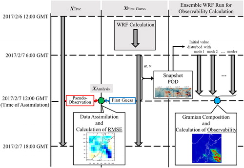
Figure 3 explains the WRF cases considered in the numerical experiment, i.e. true state, first guess for data assimilation, and an ensemble for evaluating observability Gramian. Snapshot POD is applied to the output from the first guess. The relationship of those WRF runs in time is also shown in Fig. 3.

Fig. 3. Schematic of identical-twin experiment and the calculation of observability.

3. Results

3.1. Minimum eigenvalue of empirical observability Gramian

With the conditions mentioned in Table 1 and Sections 2.5–2.6, the eigenvalues of the empirical observability Gramian in Equation (6)(6) $$\mathit{G}=\sum _{k=1}^N{\mathit{Y}}_k^T{{\mathit{R}}_k\mathit{Y}}_k,$$(6) are composed using the WRF model. In this section, the Gramian is composed point-by-point because wind observation is obtained at one grid point as in Section 2.6. Based on Equations (6)–(8), Gramian $\mathit{G}$ is obtained at each location $\lambda$(X, Y, Z). A map of the minimum eigenvalue is generated by decomposing each Gramian, and an overall trend of the observability regarding one wind observation is visualised. As explained in Section 2, we focus on the minimum eigenvalue for simplicity because it is inversely proportional to the unobservability index. In this study, the dimension of the Gramian is 4; which depends on the number of POD modes used in Equation (6)(6) $$\mathit{G}=\sum _{k=1}^N{\mathit{Y}}_k^T{{\mathit{R}}_k\mathit{Y}}_k,$$(6) .

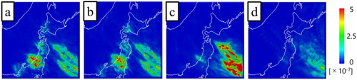
Examples of the spatial distributions of the minimum eigenvalue are shown in Fig. 4a–d. Each eigenvalue corresponds to the estimated observability of a wind observation at each point, where a large minimum eigenvalue corresponds to large observability. The east-south region seems to have higher observability, whereas terrain effects appear at low levels (Fig. 4a and b).

Fig. 4. Spatial distribution of minimum eigenvalues at each level, where (a), (b), (c), and (d) correspond to the distribution at level 2 (150 m), 7 (850 m), 12 (3200 m) and 17 (8000 m), respectively.

We now discuss the relationship between the eigenvalues and corresponding wind fields. A meteorological field can include several flow configurations, such as convection caused by pressure and temperature gradients, and the unsteady wake of terrain roughness. The eigenvalue from the empirical observability Gramian appears to have a relationship with the vertical components of the vorticity vector (${\omega }_z=\frac{\partial v}{\partial x}-\frac{\partial u}{\partial y}$) computed from horizontal wind components $u$ and $v,$ because the observability analysis evaluates the spatial and temporal changes in $u$ and $v,$ as mentioned in Section 2. Therefore, we investigate the correlation between the eigenvalue and the following three types of time-averaged vorticities (${\Omega }_{\mathrm{ave}},\mathrm{}{\Omega }_{\mathrm{pert}},\mathrm{}{\Omega }_{\mathrm{var}}$) with different time scales.

• The magnitude of the time-averaged vorticity: $${\Omega }_{\mathrm{ave}}=\left|\frac{1}{T}{\int }_T{\omega }_{i,j,t}dt\right|.$$

• The time-averaged magnitude of the perturbation component of vorticity: $${\Omega }_{\mathrm{pert}}=\frac{1}{T}{\int }_T\left|{{\omega }^{\mathrm{\text{'}}}}_{i,j,t}\right|dt,{\omega }_{i,j,t}^{\mathrm{\text{'}}}={\omega }_{i,j,t}-\frac{1}{T}{\int }_T{\omega }_{i,j,t}dt.$$

• The time-averaged magnitude of the temporal variation of vorticity: $${\Omega }_{\mathrm{var}}=\frac{1}{\mathrm{T}}{\int }_T\left|\frac{{\omega }_{i,j,t+1}-{\omega }_{i,j,t}}{\mathrm{\Delta }t}\right|dt.$$

The calculations of abovementioned three quantities are performed with the same data as the observability computation, with the setting of $T=12\mathrm{h}$ for time averaging and $\mathrm{\Delta }t=15$ min for the sampling interval. We calculated the correlation coefficient between these three domain-normalised vorticities ${\Omega }_{i,j,k}$ and the eigenvalue ${\sigma }_{\mathit{min}i,j,k}$ at level $k$ using the following equation: (20) $$\text{Corr}=\frac{E\left[\left({\sigma }_{\mathit{min}i,j,k}-E\left[{\sigma }_{\mathit{min}i,j,k}\right]\right)\left({\Omega }_{i,j,k}-E\left[{\Omega }_{i,j,k}\right]\right)\right]}{\sqrt{E\left[{\left({\sigma }_{\mathit{min}i,j,k}-E\left[{\sigma }_{\mathit{min}i,j,k}\right]\right)}^2\right]E\left[{\left({\Omega }_{i,j,k}-E\left[{\Omega }_{i,j,k}\right]\right)}^2\right]}\mathrm{}},\mathrm{}(1\le k\le 29),$$(20) where $E[-]$ calculates the expected value at level k, and ${\Omega }_{i,j,k}$ corresponds to ${\Omega }_{\mathrm{ave}},$ ${\Omega }_{\mathrm{pert}}$ or ${\Omega }_{\mathrm{var}}.$

Figure 5 shows the correlation coefficients with respect to the vertical height, the eigenvalue distributions, and the time-averaged vorticities at four levels: level 2 (150 m), level 7 (850 m), level 12 (3200 m), and level 17 (8000 m). The time-averaged magnitude of the temporal variation of vorticity ${\Omega }_{\mathrm{var}}$ (green line) has the highest correlation for all vertical levels. In contrast, the correlation with the time-averaged vorticity (${\Omega }_{\mathrm{ave}}$) is the lowest for most of the levels. The differences among these three correlations are clear below 5000 m. In this region, the correlation with ${\Omega }_{\mathrm{ave}}$ (red line) remains under 0.2, which shows almost no correlation.

Fig. 5. Correlations of the minimum eigenvalues and the actual distribution at levels 2, 7, 12, and 17. The vertical and horizontal axes correspond to the correlation coefficient and vertical height, respectively. The correlations with the time-averaged vorticity (red line), time-averaged perturbation of vorticity (blue line), and time-averaged temporal variation of vorticity (green line) are plotted. Each label on the left plot corresponds to the vorticity distributions on the right.

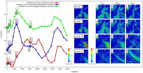
The decay of the ${\Omega }_{\mathrm{ave}}$ (red line) below 5000 m implies that the observability does not take the effect of time average of vertical vorticity z but rather their temporal changes. This results in a low correlation between the eigenvalue and ${\Omega }_{\mathrm{ave}},$ which captures the stable part. In the region influenced by the terrain, vorticity z tends to be large due to the flow unsteadiness behind hills. Figure 5c,f,i, and l show ${\Omega }_{\mathrm{ave}}$ for each level and show clearer vorticity structures from the mountains in the Japan islands and northwest region than the other vorticity metrics. On the other hand, ${\Omega }_{\mathrm{pert}},\mathrm{}{\Omega }_{\mathrm{var}},$ which do not include any time-averaged vorticity (Fig. 5a,b,d,e,g,h,j, and k), show a higher correlation with the eigenvalue.

From the above discussion, it is confirmed that the eigenvalues from this observability analysis have a strong relationship with ${\Omega }_{\mathrm{var}}.$ Therefore, the eigenvalue can be an index that indicates the unsteadiness of the flow, visualising a region where there have been large changes in the vorticity. In data assimilation, we can expect that observations at points with higher eigenvalues can effectively decrease the error of the first guess.

3.2. Application to WRF data assimilation

In this section, we verify the effect of the observability analysis on the result of WRF data assimilation. Figure 6 shows the eigenvalue distributions and RMSE changes in wind magnitude at levels 2, 7, 12, and 17. The RMSE change is defined in Equations (18)(18) $$\text{RMSE}=\sqrt{\frac{1}{N}\sum _{i=1}^N{\left(x_i-x_{i,\mathrm{}\mathit{true}}\right)}^2},$$(18) and (19)(19) $$\begin{array}{c}\text{RMSE}\text{change}\\ \text{after}\text{the}\text{assimilation}\end{array}[\%]=\frac{\text{RMSE}\text{of}\text{analysis}-\text{RMSE}\text{of}\text{first}\text{guess}}{\text{RMSE}\text{of}\text{first}\text{guess}}\times 100.$$(19) using the true state and the forecast defined in Table 2. At almost all levels, we can find the relationship between the eigenvalue and the RMSE in area A, where the RMSE decreases in the region with high observability. However, there are some exceptions, e.g. the south-west region at levels 2 and 7 (Fig. 6b and e) in area B. The eigenvalue distributions in Fig. 6, which are slightly different from those in Fig. 5, are based on the same conditions as Table 1 with the exception that the wind data until the assimilation time (2017/2/7 6:00 GMT–2017/2/7 12:00 GMT) are utilised to compose the Gramian.

Fig. 6. The distribution of eigenvalue, RMSE changes of wind magnitude, and time-averaged temporal variation of vorticity for levels 2, 7, 12, and 17, respectively. Area A shows the region where the correlation with the eigenvalue distribution is observed. Area B shows the region where RMSE reduction is observed regardless of almost zero eigenvalue. The first 6 h of the wind data (2017/2/7 6:00 GMT – 2017/2/7 12:00 GMT) are utilised to compose the Gramian.

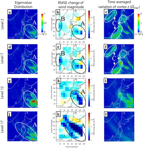
The relationship between the distribution of the Gramian eigenvalues and the RMSE changes after the assimilation is observed, because the eigenvalues are strongly related to temporal changes in vertical component of vorticity as discussed in Section 3.1. These eigenvalues visualise the unsteadiness caused by the temporal changes in the vorticity; therefore, the difference of the true state and first guess is pronounced in a high eigenvalue region as the effect of chaotic behaviours of the model. Hence, the possible error distribution can be known from the eigenvalues of the Gramian, and a forecast is improved by assimilating observations in such a region.

The exceptions at levels 2 and 7 (the area B in Fig. 6b and e) are due to the influence of domain boundaries, which can be avoided by setting the appropriate domain size for the problem of interest. The true state and first guess in this experiment use different boundary conditions generated by different re-analysis data shown in Table 2, i.e. there are large differences between both calculations near the southwest boundary that works like an inflow boundary. Assimilation of additional observations around these regions may further decrease the RMSE.

The comparison of the RMSE and ${\Omega }_{\mathrm{var}}$ shows some differences in area C of levels 2 and 7 (Fig. 6i and l). In the area, small-scale winds caused by the effect of the terrain, such as Japanese mountains and continental Asia, significantly appear. The area shows a large temporal variation in vorticity ${\Omega }_{\mathrm{var}}$ with small spatial scales. The result implies a difference between the spatial scale of a background error given in a data assimilation system ($L$ in Equation (17)(17) $$\varphi \left(s\right)=\exp (-\frac{s^2}{2L}).$$(17) ) and the spatial scale of the actual error, which is usually unknown. We set a relatively large $L$ assuming meso-scale forecasting, which is the preliminary application of the observability calculation. Thus, 3 D-VAR with such $L$ reduces the errors of meso-scale winds at high levels; however, it does not reduce small-scale errors at low levels effectively. As we mentioned in Section 1, our focus in this study is to investigate the effectiveness of target observation based on the observability Gramian, and the effectiveness is confirmed in the meso-scale WRF data assimilation.

4. Conclusion

In this study, the effectiveness of the observability Gramian for the targeted observation was investigated in the identical-twin experiment with the WRF model and 3 D-VAR, assuming a meso-scale wind prediction. There have not been prior attempts to use the observability for weather data assimilation in targeted observations.

We discussed the relationship between the spatial eigenvalue distribution of the empirical observability Gramian and corresponding wind fields. Their correlation coefficient are calculated and evaluated for levels 2, 7, 12 and 17. The correlation coefficients showed strong relationships between the eigenvalue and time-averaged magnitude of the temporal variation of vorticity ${\Omega }_{\mathrm{var}}$ when one observation was considered. This confirmed the relationship between regions with high observability and those with large unsteadiness in the wind field.

Identical-twin experiments were then conducted to investigate the effect of the observability analysis by comparing assimilation results and the eigenvalue distribution of the observability Gramian. As a result, the forecast error was effectively reduced by choosing the area with high observability as an observation location.

As for future study, we will focus more on small-scale flows in an effort to produce accurate wind prediction around a wind farm. To realise this, observability analysis will be carried out in smaller domains with large eddy simulations. Moreover, the observability of other variables (e.g. atmospheric pressure, wind speed, temperature, humidity) will be assessed. The empirical observability Gramian has the capability to evaluate the observabilities for different variables simultaneously. The eigenvalue decomposition of this Gramian considers the correlations among those variables and is expected to produce information about which variable has a large impact on a forecast.

Data availability statement

The data that support the findings of this study are available from the corresponding author, Ryoichi Yoshimura, upon reasonable request.

Disclosure statement

The authors declare no conflicts of interest.

Additional information

Funding

Insightful comments and suggestions from Dr. Nakamura of Hitachi, Ltd. are greatly acknowledged. Numerical study was performed on the supercomputer system “AFI-NITY” at the Advanced Fluid Information Research Center, Institute of Fluid Science, Tohoku University. This work was partially supported by JSPS KAKENHI Grant Number 17K17592.

References

- Baker, N. and Daley, R. 2000. Observation and background adjoint sensitivity in the adaptive observation‐targeting problem. QJR. Meteorol. Soc. 126, 1431–1454. doi:10.1002/qj.49712656511
- Barker, D. M., Huang, W., Guo, Y. R. and Bourgeois, A. 2003. A three-dimensional variational (3DVAR) data assimilation system for use with MM5. NCAR Tech Note, NCAR/TN-453 + STR, 68. pp.
- Barker, D., Huang, X.-Y., Liu, Z., Auligné, T., Zhang, X. and co-authors. 2012. The weather research and forecasting model's community variational/ensemble data assimilation system: WRFDA. Bull. Amer. Meteor. Soc. 93, 831–843. doi:10.1175/BAMS-D-11-00167.1
- Buizza, R., Cardinali, C., Kelly, G. and Thépaut, J. 2007. The value of observations. II: the value of observations located in singular‐vector‐based target areas. QJR. Meteorol. Soc. 133, 1817–1832. doi:10.1002/qj.149
- Cardinali, C., Buizza, R., Kelly, G., Shapiro, M. and Thépaut, J. 2007. The value of observations. III: influence of weather regimes on targeting. QJR. Meteorol. Soc. 133, 1833–1842. doi:10.1002/qj.148
- Carrassi, A., Trevisan, A. and Uboldi, F. 2007. Adaptive observations and assimilation in the unstable subspace by breeding on the data‐assimilation system. Tellus 59A, 101–113.
- Enomoto, S. 2006. Estimation of wind power generation using weather forecast model. Wind Energy 30, 49–56 (in Japanese).
- Kang, W. and Xu, L. 2009. Computational analysis of control systems using dynamic optimization. Available online at arXiv:0906.0215v2.
- Kang, W. and Xu, L. 2012. Optimal placement of mobile sensors for data assimilations. Tellus A: Dyn. Meteorol. Oceanogr. 64, 17133. doi:10.3402/tellusa.v64i0.17133
- Kelly, G., Thépaut, J., Buizza, R. and Cardinali, C. 2007. The value of observations. I: Data denial experiments for the Atlantic and the Pacific. QJR. Meteorol. Soc. 133, 1803–1815. doi:10.1002/qj.150
- King, S. A., Kang, W. and Xu, L. 2013. Partial observability for the shallow water equations. In: Proceedings of SIAM Conference on Control & Its Applications, San Diego, CA.
- Krener, A. J. and Ide, K. 2009. Measures of unobservability. In: IEEE Proceedings of Conference on Decision and Control, Shanghai, China, pp. 6401–6406.
- Langland, R. H. and Baker, N. L. 2004. Estimation of observation impact using the NRL atmospheric variational data assimilation adjoint system. Tellus 56A, 189–201.
- Li, H., Kalnay, E. and Miyoshi, T. 2009. Simultaneous estimation of covariance inflation and observation errors within an ensemble Kalman filter. QJR. Meteorol. Soc. 135, 523–533. doi:10.1002/qj.371
- Liu, J. and Kalnay, E. 2008. Estimating observation impact without adjoint model in an ensemble Kalman filter. QJR. Meteorol. Soc. 134, 1327–1335. doi:10.1002/qj.280
- Liu, J., Kalnay, E., Miyoshi, T. and Cardinali, C. 2009. Analysis sensitivity calculation in an ensemble Kalman filter. QJR. Meteorol. Soc. 135, 1842–1851. doi:10.1002/qj.511
- Lorenz, E. N. 1963. Deterministic nonperiodic flow. J. Atmos. Sci. 20, 130–141. doi:10.1175/1520-0469(1963)020<0130:DNF>2.0.CO;2
- Parrish, D. F. and Derber, J. C. 1992. The National Meteorological Center's spectral statistical-interpolation analysis system. Mon. Weather Rev. 120, 1747–1763. doi:10.1175/1520-0493(1992)120<1747:TNMCSS>2.0.CO;2
- Qi, J., Sun, K. and Kang, W. 2015. Optimal PMU placement for power system dynamic state estimation by using empirical observability Gramian. IEEE Trans. Power Syst. 30, 2041–2054. doi:10.1109/TPWRS.2014.2356797
- Qi, J., Sun, K. and Kang, W. 2016. Adaptive optimal PMU placement based on empirical observability Gramian. IFAC-PapersOnLine 49, 482–487. doi:10.1016/j.ifacol.2016.10.211
- REN21. 2018. Renewables 2018 global status report. Online at: http://www.ren21.net/gsr-2018/
- Sirovich, L. 1987. Turbulence and the dynamics of coherent structures, Parts I–III. Quart. Appl. Math. XLV, 561–590.
- Skamarock, W. C., Klemp, J. B., Dudhia, J., Gill, D. O. and Barker, D. M. and co-authors. 2008. A description of the advanced research WRF version 3. NCAR Tech. Note NCAR/TN-475 + STR, 113. pp.
- Toth, Z. and Kalnay, E. 1993. Ensemble forecasting at NMC: the generation of perturbations. Bull. Am. Meteor. Soc. 74, 2317–2330. doi:10.1175/1520-0477(1993)074<2317:EFANTG>2.0.CO;2
- Wang, W., Bruyère, C., Duda, M., Dudhia, J. and Gill, D. and co-authors 2017. ARW version 3 modeling system user’s guide. Mesoscale and Microscale Meteorology Laboratory, National Center for Atmospheric Research. pp. 281–282.