Improving the representation of supercooled liquid water in the HARMONIE-AROME weather forecast model

Abstract

A realistic representation of mixed-phase clouds in weather and climate models is essential to accurately simulate the model’s radiative balance and water cycle. In addition, it is important for providing downstream applications with physically realistic model data for computation of, for instance, atmospheric icing on societal infrastructure and aircraft. An important quantity for forecasts of atmospheric icing is to model accurately supercooled liquid water (SLW). In this study, we implement elements from the Thompson cloud microphysics scheme into the numerical weather prediction model HARMONIE-AROME, with the aim to improve its ability to predict SLW. We conduct an idealised process-level evaluation of microphysical processes, and analyse the water phase budget of clouds and precipitation to compare the modified and original schemes, and also identify the processes with the most impact to form SLW. Two idealised cases representing orographic lift and freezing drizzle, both known to generate significant amounts of SLW, are setup in a 1 D column version of HARMONIE-AROME. The experiments show that the amount of SLW is largely sensitive to the ice initiation processes, snow and graupel collection of cloud water, and the rain size distribution. There is a doubling of the cloud water maximum mixing ratio, in addition to a prolonged existence of SLW, with the modified scheme compared with the original scheme. The spatial and temporal extent of cloud ice and snow are reduced, due to stricter conditions for ice nucleation. The findings are important as the HARMONIE-AROME models is used for operational forecasting in many countries in northern Europe having a colder climate, as well as for climate assessments over the Arctic region.

Keywords:

• cloud microphysics
• supercooled liquid water
• numerical modelling
• HARMONIE-AROME
• atmospheric icing forecast

1. Introduction

Within numerical weather prediction (NWP) models, the main role of a cloud microphysics scheme is to create and eliminate the clouds and precipitation through numerous physical sources and sinks of water vapor, liquid, and ice and to produce their related thermodynamic effects (latent heating/cooling) that ultimately impact the model’s dynamics. However, there is a longstanding challenge in numerical weather and climate prediction to accurately represent the water-phases within the clouds, particularly at below-freezing temperatures, where many cloud microphysics schemes tend to favour production of ice species that may lead to a deficit of supercooled liquid clouds due to the Wegener-Bergeron-Findeisen effect (Fan et al. 2011). An inadequate representation of supercooled liquid water (SLW) can have consequences for forecasts of cloud cover (Ma et al. 2014), precipitation (Liu et al. 2011), and atmospheric icing (Thompson et al. 2004), as well as predictions of future climate (Tan et al. 2016). Mixed-phase clouds occur frequently in cool climate regions of mid and high latitudes (e.g., Korolev et al. 2003; Korolev and Field 2008; Furtado et al. 2016). In the Arctic region low-level liquid clouds are dominant in the radiative balance of a multiyear sea ice surface, while ice clouds are not as important (Shupe and Intrieri 2004). In this region, liquid water occur in the clouds with relatively high frequency in the winter, and can be present at temperatures as low as −34 °C and up to 6.5 km in altitude (Intrieri et al. 2002). An accurate description of mixed phase clouds in cold climates is thus of outmost importance for reliable estimates of climate change in regions where the climate is rapidly changing. Furthermore, an inaccurate description of SLW will bring considerable consequences for the overall performance of the weather and climate models, as well as for downstream applications such as modelling of icing building up on infrastructure and aviation forecasts.

Here, we seek to improve the forecasts of atmospheric icing, by modifying the cloud microphysics scheme in the NWP model HARMONIE-AROME (Seity et al. 2011; Brousseau et al. 2016; Bengtsson et al. 2017), used for regional, high-resolution operational weather forecasts in 10 European countries, as well as for climate change assessments over northern Europe and the Arctic region. The use of this model in the present study ensures that the improvement found in predicting SLW, can be easily transferred into operational weather forecasts in Nordic countries where an improved description of mixed-phase clouds benefits the forecast accuracy of icing on the natural environment as well as ground infrastructure that could cause monetary damage to industry/society as well as human safety.

The cloud microphysics scheme in HARMONIE-AROME, called ICE3, is based on physics that can be traced back to Lin et al. (1983). A study by Liu et al. (2011) compared several cloud microphysics schemes and their ability to simulate the amount of SLW. They concluded that the schemes based on physics similar to that of Lin et al. (1983) had a poor representation of the SLW, which was considerably improved in the cloud microphysics schemes presented in Morrison et al. (2009) and Thompson et al. (2008) (hereafter T08). Their study found that the main microphysical processes contributing the improvements seen in SLW were attributed to better descriptions of ice initiation - the Lin et al. (1983) type schemes were too rapid to initiate ice from vapor when ice supersaturation is reached, or would freeze water droplets prematurely. Another aspect found was the improved conversion pathways to graupel where the T08 and Morrison et al. (2009) schemes use a variable collection efficiency following Wang and Ji (2000), instead of the unity efficiency of snow-collecting cloud water as used in the Lin et al. (1983) type schemes. In a separate study, Nygaard et al. (2011) compared three different microphysics schemes available in the Weather Research and Forecasting (WRF) model, and their ability to predict in-cloud icing at ground level, and concluded that T08 had the most accurate values of SLW.

The T08 cloud microphysics scheme is a bulk microphysical parameterisation that has been developed for the WRF model. It has been implemented and tested in many NWP models including the fifth-generation Pennsylvania State University–National Center for Atmospheric Research Mesoscale Model (MM5), the Rapid Refresh (RAP), and the High-Resolution Rapid Refresh (HRRR) model. One of the main goals in the development of the T08 scheme was to improve forecasts of water phase, in particular to support aviation applications to forecast aircraft icing.

In this study, we seek to improve the representation of SLW in the NWP model HARMONIE-AROME by implementing elements of the T08 microphysics scheme. We carefully assess the performance of the T08 scheme in a single column version of HARMONIE-AROME by conducting a very idealized process level evaluation, where we look at how the water phase changes due to modifications in the cloud and precipitation process formulations, to highlight key processes necessary for modelling SLW.

2. Methodology

HARMONIE-AROME is a convection-permitting NWP model. It is based on the AROME model (Seity et al. 2011; Brousseau et al. 2016), which is developed by Météo-France and partners in the ALADIN consortium (Termonia et al. 2018). The collaboration between the ALADIN and HIRLAM consortium consisting of the national weather services in 26 countries in Europe and northern Africa, is responsible for the development and maintenance of HARMONIE-AROME (Bengtsson et al. 2017).

ICE3 is the existing HARMONIE-AROME one-moment bulk microphysics scheme with prognostic variables for the mass of cloud water, rain, cloud ice, snow, and graupel, including physical processes mostly based upon Cohard and Pinty (2000a, 2000b), for which many aspects can be traced back to Lin et al. (1983), Rutledge and Hobbs (1984), and Ferrier (1994). Some changes were implemented to the scheme in 2014, hereafter referred to as the OCND2 option (Müller et al. 2017). These changes were motivated by an underestimation of low-level SLW clouds, and an over-abundance of near ground level ice clouds when T < −20 °C, along with an excess of cirrus clouds. All were linked with a general over prediction of cloud ice. The OCND2 option contained changes to the parameterisation of vapor deposition and sublimation of cloud ice and snow, the collection efficiency between snow/graupel and cloud water, accretion of cloud droplets by rain, autoconversion, ice-cloud cover, and modifications of the IN-concentration for heterogeneous ice nucleation. The implementation of OCND2 led to a better representation of mixed-phase clouds, as well as improved forecasts of 2-m temperature and relative humidity during wintertime (Bengtsson et al. 2017). However, comparisons with microwave radiometer and vertically pointing cloud radar observations indicate that, even though there was an improvement in the partitioning between cloud water and ice, there was still an underestimation of SLW even with the OCND2 option included (see e.g. Fig. 1 in Bengtsson et al. 2017).

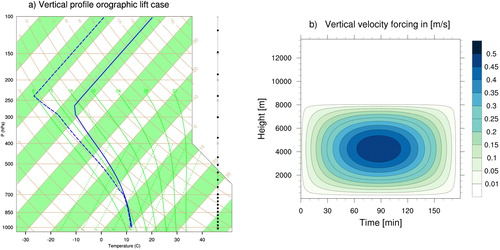
Fig. 1. (a) Skew-T plot of the initial profile and (b) time-height cross-section of the vertical velocity forcing used for the orographic lifting case in MUSC.

2.1. Experimental set-up

A single column version of HARMONIE-AROME, called Modèle Unifié, Simple Colonne (MUSC) is the basis for this study. This provides an efficient way for testing the sensitivity of various microphysical assumptions, production, and depletion terms in an idealised environment. Furthermore, the results are usually easy to interpret as it is possible to isolate the effects of the microphysical sensitivities from typically confounding feedbacks by the turbulence, radiation, or boundary layer parameterisations, as well as the dynamical feedbacks of a full 3 D real world simulation. In our simulations MUSC is run with 60 vertical levels, with approximately 10-m spacing near the surface stretched to a few kilometres spacing near the model top. In addition, given the simplicity of 1 D column models, the output of many variables as well as microphysical processes can be performed each time step since this is easily manageable compared to 2 D and 3 D simulations.

We constructed a set of idealised experiments based on initial profiles of temperature, pressure, and water vapor from prior similar work related to idealised case studies together with prescribed forcing of vertical velocity. All other physical parameterisations were switched off with only the microphysics scheme being active. A time-step of 60 s was used since that is the setting used in the reference configuration of the model, and our own tests with shorter time-steps showed similar results. The first case presented below is a simple orographic lift case based on prior simulations using the Weather Research and Forecasting (WRF) model by Thompson et al. (2004, 2008) and Thompson and Eidhammer (2014). The second case features an idealised version of a high-impact freezing drizzle case that occurred in and around Oslo, Norway on Jan 15, 2018.

2.1.1. Orographic lift case

This idealised case was created to mimic a cloud parcel being lifted by the orography of a simple bell-shaped hill, similar to the WRF experiments of Thompson et al. (2004). In contrast to their simulations in two dimensions, MUSC approximated the orographic lift using a simple sinusoidal in space/time prescribed vertical velocity. The velocity forcing term was applied in 5-minute intervals in the altitude range of 250 to 8000 m with a maximum magnitude of 0.5 m s⁻¹ applied near 4000 m at the mid-point (90 min) of the 3-h total simulation time (Fig. 1b). The initial vertical atmospheric thermodynamic profile (see Fig. 1a) was taken from the Improvement of Microphysical Parameterization through Observational Verification Experiment (IMPROVE-2) case, which has been used in other scientific studies, e.g. Stoelinga et al. (2003). This profile rapidly saturates just above the ground and remains nearly neutral moist statically stable and up to 700 hPa, where the relative humidity is gradually reduced though remains effectively at ice saturation values. With the relatively weak updraft, we expect this case to create significant amounts of SLW.

2.1.2. Freezing drizzle case

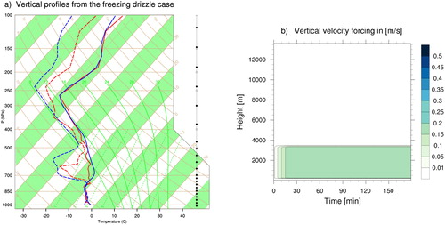
On Jan 15, 2018, a severe icing event occurred in the region around Oslo, Norway including major impacts to flight operations at Oslo International Airport. The operational model forecasts out of Norway did not generate the observed conditions of freezing drizzle/rain, but instead predicted solid precipitation (snow). A radiosonde was launched by MET-Norway personnel at Blindern, Oslo, at 1050 CET. The temperature profile showed a common freezing drizzle situation with all sub-zero temperatures and saturated conditions up to near -12 °C and a very obvious temperature inversion above. This temperature and humidity structure is often found in freezing drizzle events as it is believed that ice is difficult to form at these relatively warm temperatures without the nearly saturated conditions extending higher up into lower temperature altitudes.

A plot of the radiosonde data and the corresponding operational model-predicted sounding is shown in Fig. 2. HARMONIE-AROME produced a very similar profile of temperature and humidity that was obviously smoother than the true sounding. The smooth model sounding was therefore used as the thermodynamic profile in the MUSC idealised simulation of this case. Within MUSC, we applied a constant forcing of 0.2 m s⁻¹ to the model levels between 250 and 3500 m (the base of the inversion).

Fig. 2. (a) Skew-T plot of the freezing drizzle case, blue lines represent the operational forecast from HARMONIE-AROME and initial profile used in MUSC, while red lines represent the radiosonde profile taken from MET-Norway’s site at Blindern, Oslo at 1150 UTC. (b) time-height cross-section of the vertical velocity forcing applied to the MUSC experiments for the freezing drizzle case.

3. Experiments and results

In both idealised MUSC cases, we studied several processes thought to be important to the production or depletion of supercooled liquid water. An abbreviated summary of the experiments with brief explanation of the microphysical processes altered is listed in Table 1. More details of individual experiments and the differences between them are mentioned in the following sections. Due to myriad feedbacks of the various microphysical processes, it is not always easy to foresee the outcome of changing certain parameters or treatments. Furthermore, singular individual code changes performed one at a time is not necessarily useful and the number of total permutations would be quite large, therefore, we combine one change upon the next as listed in Table 1. Another justification for combining the changes is the overall intent to produce results consistent with those using the T08 WRF microphysics scheme in order to suppress ice production at relatively warm temperatures to permit more supercooled liquid water.

Table 1. List of MUSC 1 D experiments and the microphysical processes studied.

Experiment	Process altered	Previous	New
CTRL	Heterogeneous ice nucleation	Code mistake	Bug fix
BR74	Autoconversion (cloud to rain)	Khairoutdinov and Kogan (2000)	Berry and Reinhardt (1974)
ACC	Rain accreting cloud water	Variable efficiency (OCND2)	Variable efficiency (Thompson)
C86	Heterogeneous ice nucleation	Meyers et al. (1992)	Cooper (1986)
Bigg	Freezing of water drops	None	Bigg (1954)
GCW	Graupel collecting cloud water	Ferrier (1994) for dry growth; Musil (1970) and Nelson (1983) for wet growth	Cober and List (1993)
SCW	Snow collecting cloud water	Farley et al. (1989)	Wang and Ji (2000)
RCS	Rain collecting snow	Ferrier (1994); Eff = 1.0	New variable collection efficiency
RCG	Rain collecting graupel	Ferrier (1994); Eff = 1.0	New variable collection efficiency
HP	Hydrometeor properties	Locatelli and Hobbs (1974)	Thompson et al. (2008)
Y-INT	Rain inverse exponential Y-intercept parameter	8 × 10^6 m^−4 (Marshal-Palmer)	Variable intercept parameter (Thompson et al 2004)

3.1. Orographic lift case

3.1.1. Control experiment (CTRL)

The original HARMONIE-AROME cycle40h1 code with the OCND2 option active contained a coding error that prevented any new heterogeneous ice nucleation from occurring until a non-zero amount of cloud ice was already present, which was only possible by homogeneous freezing of water drops at T < -38 °C. This code error was found during construction of the various experiments and subsequently corrected so that all results shown below for the ‘control’ experiment include this fix and thus deviate from the operational code from the outset. Correcting the error naturally caused more typical heterogeneous ice nucleation rates and consequently a drastic increase in cloud ice at all sub-zero temperatures, making the corrected OCND2 version of the microphysics scheme extremely ‘ice friendly’.

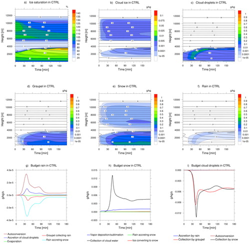
In order to visualise the results of the control experiment followed by the suite of sensitivity experiments listed in Table 1, an overview of the control run is provided in Fig. 3 showing time-height cross-sections of the microphysics species and their respective sources and sinks. Note in particular how all areas with higher than 100% relative humidity with respect to ice (RH_ice > 100%) immediately have corresponding cloud ice mass mostly due to primary nucleation of ice from vapor deposition (Fig. 3b). The OCND2 option for ice nucleation is a modified form of Meyers et al. (1992) that requires only ice supersaturation and T < 0 °C. This clearly makes prolific ice that easily grow larger via continued vapor growth supplied by the prescribed updraft velocity. As the updraft velocity gradually increases, there is enough lift and slow enough ice growth that water saturation is achieved and cloud droplets form and increase for the first hour (Fig. 3c); however, after sufficient ice and snow growth, the cloud water is depleted by riming of snow and formation of graupel and subsequent riming of graupel (Fig. 3i), effectively glaciating most of the cloud. The ice particles fall to the level of melting to become rain below.

Fig. 3. Results from the control run (CTRL) for the orographic lift case. Time-height cross-sections of (a) relative humidity with respect to ice saturation, mixing ratios of (b) cloud ice, (c) cloud droplets, (d) graupel, (e) snow, and (f) rain. Budget plots with time-evolutions of the sum of sources and sinks for (g) cloud ice, (h) snow, and (i) cloud droplets.

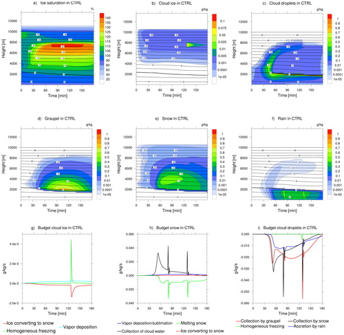
By closely inspecting the budgets of cloud ice, snow, and cloud water (Fig. 3g–i), a number of notable sharp maxima in source and sink terms help to explain the microphysical evolutions far better than a real-world case study with all its interactions of full dynamics and other physical parameterisations. For example, the maximum of cloud ice in Fig. 3b) near 120 min at 8000 m altitude is explained by the lofting of cloud droplets to the homogeneous freezing level, producing a sharp increase in the budget of cloud ice at the corresponding time. Since a large portion of the ice converts to the snow category, there is a small increase shown in the corresponding snow panel (Fig. 3e).

Another series of spikes in the budget of snow and cloud water (also rain, not shown) is evident in Fig. 3h,i in which there is a gradual build-up of cloud water content immediately adjacent to the melting level until the times of 80 and 130 mins when a sudden burst of snow growth occurs due to riming that rapidly depletes the cloud water. Those rapid snow growth rates correspond to the two maxima shown in rain as the snow falls below the melting level seen in Fig. 3f. Such rapid jumps in microphysics source or sink terms clearly represent unphysical behaviour and require further investigations. Two sensitivity experiments discussed below address how choices in heterogeneous ice initiation affected the overall cloud structure. For this sensitivity experiment we do not address the two warm rain experiments for autoconversion (BR74) and accretion (ACC), as they did not impact the orographic lift case notably. They are discussed in more detail in the freezing drizzle case, where the impact was higher.

3.1.2. Ice initiation experiments (C86 and Bigg)

As mentioned earlier, the scheme’s primary heterogeneous ice nucleation is through vapor deposition using the modified Meyers et al. (1992) formulation (OCND2 option). As reported in Thompson et al. (2004), the Meyers method produces numerous ice crystals at all ice supersaturations and T < 0 °C. In contrast, the T08 scheme in WRF greatly restricts the initiation of cloud ice, since studies of supercooled liquid water clouds and aircraft icing as well as cloud chamber laboratory tests indicate how rarely ice forms in the real atmosphere between 0 and approximately -12 °C unless water drops form first. Specifically, the T08 scheme requires ice supersaturation to reach at least 125% or be water saturated and T < -12 °C before nucleating ice with a concentration following the observations of Cooper (1986). We implemented this approach into HARMONIE-AROME, and also added a diagnostic calculation of the ice number concentration based on the mass and temperature (Kristjánsson et al. 2000). The latter was necessary because the sublimation and vapor deposition method downstream in the code, was designed specifically for Meyers ice nucleation, and would not work with Cooper lest the ice number concentration was diagnosed in addition. This sensitivity experiment is called C86.

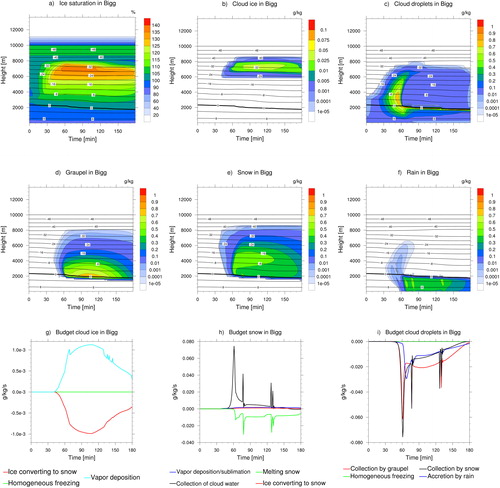
In addition to C86, and since the original scheme did not explicitly account for immersion freezing of existing water drops, we also included Bigg (1953) heterogeneous freezing of water. This treatment also follows the T08 scheme with 100 size bins of cloud water and rain drops to form a look-up table of fraction of drops that freeze as a function of volume of water drop and temperature. The combined results of C86 and Bigg immersion freezing is shown in Fig. 4. The starting time and magnitudes of all ice species (cloud ice, snow, and graupel) changed dramatically with this combination, as well as the resulting supercooled water. The changes produced a delay in ice initiation and subsequent growth to snow and permits a larger build-up of cloud water. However, the glaciation of the upper parts of the cloud eventually look qualitatively similar to the original control run, and the added cloud water combined with snow (riming) produces overall slightly more graupel than control. The larger values of cloud water also lead to slightly more conversion to rain and a number of previous spikes in the source/sink terms were eliminated, except the snow collecting cloud water.

Fig. 4. Results from the Bigg experiment for the orographic lift case. Time-height cross-sections of (a) relative humidity with respect to ice saturation, mixing ratios of (b) cloud ice, (c) cloud droplets, (d) graupel, (e) snow, and (f) rain. Budget plots with time-evolutions of the sum of sources and sinks for (g) cloud ice, (h) snow, and (i) cloud droplets.

3.1.3. Cloud water collection experiments (SCW and GCW)

Similar to when rain collects (accretes) cloud droplets, when snow or graupel fall through a liquid cloud, some droplets are collected and freeze onto the ice particle in a process known as riming. When additional riming on graupel occurs, the result is a simple increase in the mass of graupel and corresponding loss in cloud water. However, when snow rimes, the result can be either a mass increase in snow or newly formed graupel, or a combination of the two. The existing ICE3 microphysics scheme uses thresholds for snow and cloud water content following Rutledge and Hobbs (1984) to decide whether the rimed mass contributes to graupel or increased snow content. In the ICE3 scheme a threshold diameter of 7 mm for snow resulted in 100% graupel production from riming, otherwise snow content increased. Similar to other changes mentioned previously, the treatment of snow riming to form graupel was switched to follow the T08 scheme in which a ratio of snow riming to depositional growth is calculated and a percentage of riming is applied to form new graupel while the remaining percentage contributes to growth of snow content. This represents a smooth, linear function rather than the step-function behavior of the original ICE3 scheme.

In addition, the ICE3 (OCND2) scheme uses a variable collection efficiency of snow collecting cloud water, based on a characteristic diameter of cloud droplets. Many prior schemes (e.g., Rutledge and Hobbs, 1984; Reisner et al. 1998) uses a collection efficiency of unity, but the scheme diagnostically determines the efficiency based on Lohmann (2004). Meanwhile, as mentioned earlier, the T08 scheme calculates the efficiency following Wang and Ji (2000) in which the characteristic diameter of snow/graupel as well as cloud droplets are considered. So, besides changing the decision of how much snow riming results in graupel formation, the riming efficiency calculation was changed as well. There is also a temperature dependence within the ICE3 scheme, that prevents graupel and snow from collecting cloud droplets when T > 0 °C. We removed this dependency as these processes should also be possible within the melting layer.

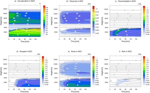
The most notable impact of changing to new riming collection efficiencies and graupel production, is an increase in the maximum cloud water content that dissipates more gradually with time (see Fig. 5c). Initially there is an increase to graupel content, followed by a rapid dissipation. The snow content experiences the opposite effect with a more gradual build up, so the last half of the simulation is dominated by snow and much less graupel. The higher amount of graupel at earlier lead-times in this experiment compared to the previous, is likely an effect of the now linear function of snow riming to form graupel and subsequent collection of cloud water by faster falling graupel. In the previous experiment (Bigg) with the original ICE3 parameterization, the threshold of 7 mm snow size before converting to graupel, likely slows the initial graupel creation. In the latter half of the simulation of SCW, when snow growth dominates, the collection efficiency was reduced compared with CTRL resulting in lower conversion to graupel. The temperature dependence has the effect of an on/off switch for graupel and snow collecting cloud droplets near the melting layer. Cloud water builds up where T > 0 °C, and is quickly collected by snow and graupel when the temperature falls below freezing. By removing this dependence, we eliminated the spikes of cloud water depletion by snow riming (recall Fig. 4i) as seen near the melting level of Fig. 4c that are no longer found in Fig. 5c.

Fig. 5. Results from experiment SCW for the orographic lift case. Time-height cross-sections of mixing ratios of (a) relative humidity with respect to ice saturation, mixing ratios of (b) cloud ice, (c) cloud droplets, (d) graupel, (e) snow, and (f) rain. Budget plots with time-evolutions of the sum of sources and sinks for (g) rain, (h) snow, and (i) cloud droplets.

Some odd wiggle-like features in the rates of ‘collection of cloud water’ and subsequently ‘snow melting’ appear in the budget plot of snow (Fig.5h). This is due to the division into snow or graupel as the resulting hydrometeor, when snow collects cloud water.

3.1.4. Rain collecting snow/graupel experiments (RCG and RCS)

Similar to the snow riming process, when rain collides with snow, the result could be considered graupel, or it might just increase the mass of snow, depending on the size of the water drop being collected. This decision can be somewhat critical as there are many pathways to create graupel, which has significantly higher assumed density and terminal velocity, often 2-5 times the values for snow. Schemes that favour graupel production have a very high precipitation efficiency as compared to those that slow the production of graupel and favour the snow or cloud water categories (Liu et al. 2011), because these slower-falling species will remain longer in the atmosphere.

The original ICE3 scheme treatment of rain collecting either snow or graupel following Ferrier (1994) was retained, however, the collection efficiencies were modified to take into account the possibility that small drizzle drops fall slowly. The continuous collection equation (see e.g., Verlinde et al. 1990) has a double-integral that includes the difference of particle velocity between collector and collected species. This obviously trends toward zero if the fallspeed of the rain and snow are nearly the same, which does occur with small drizzle (∼200 μm) and medium to large snow (∼5 mm). The T08 scheme resolves this problem by pre-calculating the explicit double integral using 100 size bins of each species with their proper respective velocities and applying the look-up table during model run time. In this work, we decided to apply a far simpler method of calculating the mass-weighted mean size of each species, rain and snow. We then used their mean diameter to calculate the corresponding terminal velocity using the usual power-law constants and took their ratio. As this terminal velocity ratio approaches unity, the collection efficiency should be very near zero, whereas whenever one species is falling much faster than the other, the collection of these two particle types should be large. A sinusoidal form with minimum (maximum) of 10% (90%) efficiency was applied to the velocity ratio as shown in Fig. 6.

Fig. 6. Plot of the collection efficiency for rain collecting snow/graupel with terminal velocity ratio (snow/graupel to rain).

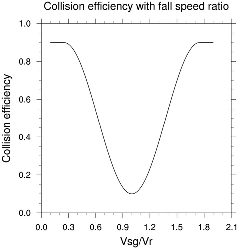
The treatment of rain and graupel collisions is simpler than rain-snow since it does not result in a new category being formed, but we applied the same technique of variable collection efficiency based on mass-weighted mean size of rain and graupel and resulting terminal velocity ratio. The combined results of these two code alterations showed very little overall sensitivity and are not shown.

3.1.5. Hydrometeor properties experiment (HP)

Most microphysics schemes utilise a power-law relationship for mass and velocity as a function of particle diameter of the form: $m\left(D\right)={aD}^b$ and $v\left(D\right)={cD}^d,$ where m is mass, v is velocity, D is diameter and a, b, c, and d are constants found in Table 2. T08 clearly showed that snow density is an inverse function of diameter, which is why that scheme assumes ‘plate-like’ snow with b = 2. Many different microphysics schemes have different values for these power law constants, and we experimented with changing the original values in ICE3 based on Locatelli and Hobbs (1974) to use the T08 constants as summarised in Table 2. The snow terminal velocity is decreased compared to control for D < 600 μm and increased for larger D.

Table 2. List of coefficients for mass and velocity-diameter relations for CTRL and HP experiments.

Species	CTRL	HP
Snow	a = 0.02, b = 1.9, c = 5.1, d = 0.27	a = 0.069, b = 2, c = 40, d = 0.55
Graupel	a = 19.6, b = 2.8, c = 124, d = 0.66	a = 19.6, b = 2.8, c = 442, d = 0.89

The resulting sensitivity experiment (not shown) produced a slight increase in cloud water content and decrease in overall snow content, due to the overall slower falling snow collecting less rime. The increased cloud water permits a slight increase in supercooled rain (from autoconversion and accretion) as well. This minor increase of rain content and mean size causes a slight increase in graupel content as well, since slightly larger rain drops have a higher probability of freezing using the Bigg (1953) immersion freezing method.

3.1.6. Rain Y-Intercept experiment (Y-INT)

The existing ICE3 scheme is similar to nearly all other one-moment microphysical parameterisations in the treatment of assumed rain size distribution following Marshall and Palmer (1948) as this distribution is often used in models since Lin et al. (1983). That is, the Y-intercept parameter (hereafter referred to as N₀) of the inverse exponential distribution is set constant to 8 x 10⁶ m⁻⁴. This value has often been validated from time averaging of disdrometer data, especially from melting ice particles. However as far back as Waldvogel (1974), who coined the term ‘N₀ jump’, it has been recognised that the value is not often constant and can be much larger in the case of warm-rain (drizzle) processes than for melting snow, as the prior tends to represent more small drops. It is for this reason that Thompson et al. (2004) decided to implement a diagnostic calculation of the N₀ parameter through inspecting the vertical column of rain and ice. More specifically, if rain is found below a melting layer, it is assumed that the rain was produced by melting of snow and/or graupel, which will result in large raindrops and a smaller intercept parameter. If there is no ice above the melting layer, the intercept parameter can be up to two orders of magnitude larger to simulate drizzle. In our implementation of this idea into the ICE3 scheme, we greatly simplified the diagnosis of rain intercept parameter by simply setting its value to the legacy constant for T > 0 °C and two orders of magnitude larger when T <−2 °C with a smooth transition in between using the formula: $N_0=8\mathrm{*}{10}^{\left(6-T\right)},$ where T is temperature (C) and N₀ has units of m⁻⁴. Our rationale for simplifying this treatment as compared to Thompson et al. (2004) is that rain present when T <−2 °C most likely stem from collision-coalescence processes, and not melted snow or graupel. However, without the check for ice above melting, this method will not work well in cases of warm-rain (drizzle) in above melting temperatures. Rain produced by melting ice species that fall through a layer of subzero temperatures below the melting layer, will also be treated as drizzle. Therefore, a future research path will be to adjust our methodology to match more closely what is done in Thompson et al. (2004). Regardless, the diagnostic calculation of intercept parameter affects all subsequent rain-related source and sink terms including the terminal velocity of the rain, which is expected to have a substantial sensitivity.

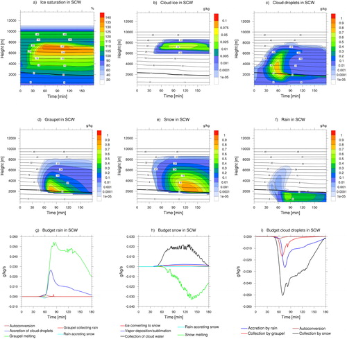
The final result of the entire suite of the 10 model changes listed in Table 1 is found in Fig. 7. The cloud droplets maximum mixing ratio is slightly higher than for the HP experiment, yet it takes longer to deplete the cloud water, especially for values less than 0.3 g kg⁻¹. The budget plot for cloud droplets (Fig. 7i) shows a reduced rate of accretion by rain, which is expected when the mean size of rain drops is much smaller. Collection of cloud droplets by snow is decreased in the first part of the simulation, but increased in the latter half. Graupel maximum mixing ratio is reached later in the simulation, most likely due to more cloud water available. Low mixing ratios of rain remain longer at T < 0 °C, as the drops are small enough to avoid efficient collection by snow and graupel. The maximum mixing ratio of snow is reduced compared with the previous experiment (HP), and, similar to graupel, happens later in the simulation.

Fig. 7. Results from the Y-INT experiment for the orographic lift case. Time-height cross-sections of (a) relative humidity with respect to ice saturation, mixing ratios of (b) cloud ice, (c) cloud droplets, (d) graupel, (e) snow, and (f) rain. Budget plots with time-evolutions of the sum of sources and sinks for (g) rain, (h) snow, and (i) cloud droplets.

3.2. Freezing drizzle case

3.2.1. CTRL

Besides the orographic lift case, we wanted to ensure how the original and newly updated physics would perform in a case of observed freezing drizzle, as described in the methodology. The control simulation (CTRL) (Fig. 8) shows cloud water building up below the inversion during the first 30 minutes, before it is reduced again, leaving only a narrow band of relatively high mixing ratios of cloud water just below the cloud top. The reduction in cloud water correlates with an increase in snow (Fig. 8e) and graupel (Fig. 8d), and can be seen as a clear spike in the rates of graupel and snow collecting cloud water (Fig. 8i). These processes quickly glaciate the cloud, and only a small amount of cloud droplets remain afterwards.

Fig. 8. Results from the control experiment (CTRL) for the freezing drizzle case. Time-height cross-sections of (a) relative humidity with respect to ice saturation, mixing ratios of (b) cloud ice, (c) cloud droplets, (d) graupel, (e) snow, and (f) rain. Budget plots with time-evolutions of the sum of sources and sinks for (g) rain, (h) snow, and (i) cloud droplets.

Much of the initial profile is saturated with respect to ice (Fig. 8a), resulting in ice initiation both in the upper levels of the column and below the inversion, making the lower cloud a mixed phase cloud from the beginning (Fig. 8b). Cloud ice quickly grows into snow, that can be found throughout both clouds. The lack of cloud water in the upper cloud, indicates that the only source of snow is cloud ice conversion and vapor deposition for further growth. The upper ice cloud could possibly create a condition of ‘seeder-feeder’ of ice falling into a supercooled liquid water cloud (Thompson and Eidhammer 2014), but the layer between is dry enough for all ice particles to sublimate before reaching the lower cloud. All ice particles present in the lower cloud must therefore have been generated there. Freezing drizzle can be found in the areas with the highest cloud water amounts, but only at very low mixing ratios (less than 0.001 g kg⁻¹), and it does not reach the surface. The rain budget plot in Fig. 8g, shows that the drizzle drops are removed by graupel and snow collection almost as quickly as it is being generated by autoconversion and accretion. The low autoconversion and accretion rates are probably due to the low amounts of cloud water. Similar to the orographic lift case, cloud ice is introduced early in CTRL even though the cloud top temperature is approximately –12 °C. The ice crystals quickly convert into snow, and the snow starts to collect cloud water that introduces graupel. Snow and graupel then collect most of the remaining liquid, inhibiting freezing drizzle and favouring precipitation as snow, contrary to the observations from which this idealised case is based upon.

3.2.2. Rain experiments (BR74 and ACC)

The physical process of droplet collision-coalescence is responsible for the so-called ‘warm-rain’ process (in contrast to ice particles melting into rain drops) while most numerical models use the term of autoconversion to parameterise this process. The OCND2 option uses the autoconversion parameterisation of Khairoutdinov and Kogan (2000; hereafter KK00) to convert cloud water to the rain category. A known potential problem with the KK00 method is that any non-zero amount of cloud water can initiate small values of rain, regardless of the size or amount of cloud water whereas other methods of converting cloud water to rain require threshold diameters or minimum amount of cloud water before starting the conversion. Therefore, one of the first changes to the scheme was switching to the Berry and Reinhardt (1974; hereafter BR74) method that utilises three different characteristic diameters of the cloud water distribution, which can account for more complex treatments of the shape of the cloud water spectra as discussed in T08. Similar to T08, the assumed cloud droplet number concentration was set to 100 cm⁻³ for all sensitivity experiments performed, however, the fully 3 D HARMONIE-AROME model has settings of 100, 300 and 500 cm⁻³, respectively, for maritime, continental, and urban points.

Besides autoconversion, another warm rain process by which falling rain drops collide and collect with the small cloud droplets, referred to as ‘accretion’ was altered in a sensitivity experiment. The original code basically used the Wisner et al. (1972) assumption that rain falls much faster than cloud water which greatly simplifies the mathematical double-integral of the full collection equation. However, instead of using a constant collection efficiency, the scheme uses a variable efficiency that is diagnosed from the mean size of the cloud droplets. In another warm rain sensitivity experiment, the collision efficiency of rain collecting cloud water was changed to match the T08 method in which both the median volume diameter of rain and cloud water is computed using 100 size bins of each category and a look-up table of collection efficiency following Hall (1980) was created. Since the efficiency is typically very high regardless of method, the sensitivity test called ACC showed only minor differences from BR74. However, the role of autoconversion is potentially very important because it can act as a ‘trigger’ to increase (decrease) rain (cloud water) further via accretion.

The results from this experiment are shown in Fig. 9. In the control experiment, rain is produced at the second time step (120 s), while in ACC, rain does not form before 29 minutes into the simulation. The results showed that the BR74 parameterisation allows slightly more supercooled cloud water to build up before the cold processes start to glaciate the cloud (Fig. 9c). Less cloud water is converted into drizzle, and a little more snow is generated in ACC, which is due to more cloud water available for the riming process. An interesting effect is that the graupel production is delayed by approximately 25–30 minutes, showing that the generation of graupel is more sensitive to the amount of rain drops than cloud droplets.

Fig. 9. Results from the ACC experiment for the freezing drizzle case. Time-height cross-sections of (a) relative humidity with respect to ice saturation, mixing ratios of (b) cloud ice, (c) cloud droplets, (d) graupel, (e) snow, and (f) rain.

3.2.3. Ice initiation experiments (C86 and Bigg)

As in the orographic lift case, the ice initiation processes (not shown) have the strongest impact on the results. Ice supersaturation is easily obtained (requirement for ice initiation for Meyers), yet 125% ice supersaturation (requirement for Cooper in T08) is only achieved after 90 minutes near the cloud top. This is generated due to the cold temperatures, and appears only below -12 °C. As such high supersaturation is not achieved in the upper part of the column, the entire upper ice cloud is removed by this change. While ice supersaturations are low to moderate (near RH_ice = 115%), ice is not immediately formed with the new modifications, however, real world weather conditions in this case could have upper-altitude frontal lift that would supply additional vertical velocity to increase RH_ice further until ice would occur. Such lack or presence of the high-altitude ice cloud would clearly impact both cloud cover and radiation, and have large feedbacks in a real forecast. The late onset of cloud ice after modifying the scheme also delays the generation of graupel and snow, which in return allows larger amounts of cloud water to build up. More cloud water is allowed to convert into the rain category, and now it reaches the surface.

3.2.4. Liquid water collection experiments (GCW, SCW, RCS, and RCG)

The rates of graupel and snow collecting cloud water are substantially reduced in GCW and SCW (not shown). The result is that cloud water now dissipates more gradually, so cloud water is kept above 0.1 g kg⁻¹ for more than 30–40 minutes after reaching the maximum value, which is in agreement with the results seen in the orographic lift case. Before this change, the same reduction took only about 5 minutes. In addition, larger amounts of cloud water remain in the middle layer of the cloud (between 1000 and 2500 m). With larger amounts present, more cloud water becomes drizzle in this layer. We also see an increase in the snow mixing ratio, especially near the surface. The maximum mixing ratio of snow is shifted to later in the simulation, consistent with the orographic lift case. It was not possible to detect any changes in the results due to rain collecting graupel or snow, except for slightly lower rates, due to very low amounts of rain in this experiment.

3.2.5. Hydrometeor properties experiment (HP)

The increased snow maximum from the collection experiments is reduced also in this case with the updated hydrometeor properties (not shown). As discussed previously this is due to less riming of cloud water with slower falling snow. Subsequently, the amounts of cloud water, graupel and drizzle are slightly increased in this experiment.

3.2.6. Rain Y-intercept experiment (Y-INT)

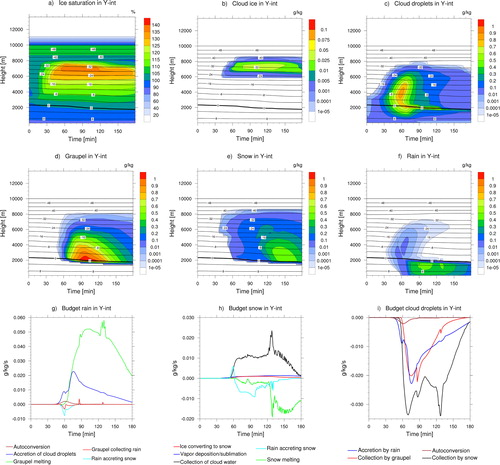
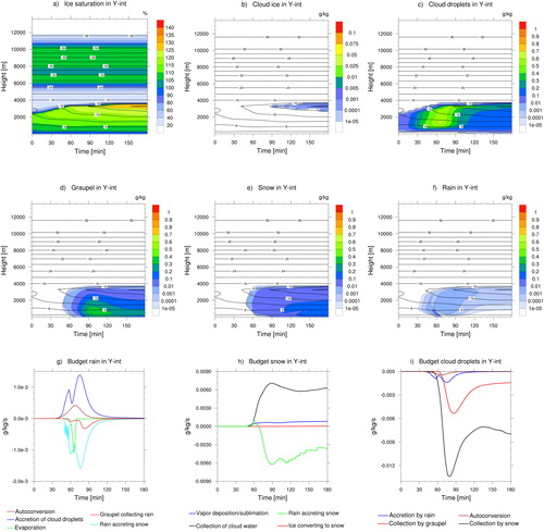
Results from the full suite of code modifications is found in Fig. 10. The variable N₀ is assumed to be very important for this case, as all the raindrops are created by warm processes (accretion and autoconversion), meaning that the constant value from Marshall and Palmer (1948) will lead to a distribution of too few and large raindrops, compared with what we would expect from drizzle drops. The smaller raindrops in this simulation lead to a higher concentration of cloud droplets and rain, as fewer drops are being captured by snow (a clear reduction in the rates in Fig. 10h), leading to less snow. Graupel on the other hand is slightly increased. This increase is mostly due to an increase in the amount of rain and snow collection that become graupel (not shown).

Fig. 10. Results from experiment Y-INT for the freezing drizzle case. Time-height cross-sections of (a) relative humidity with respect to ice saturation, mixing ratios of (b) cloud ice, (c) cloud droplets, (d) graupel, (e) snow, and (f) rain. Budget plots with time-evolutions of the sum of sources and sinks for (g) rain, (h) snow, and (i) cloud droplets.

4. Discussion and conclusion

In this study, we have modified the cloud microphysics scheme in HARMONIE-AROME to resemble the T08 scheme, in order to improve the representation of SLW. Two idealised 1 D test cases were constructed to represent orographic lifting and freezing drizzle, to validate the new scheme. Comparing the results from CTRL (Fig. 3) to Y-INT (Fig. 7), shows a big difference for the orographic lift case. Maximum cloud droplet mixing ratio where T < 0 °C is doubled, and the time it takes to reduce the mixing ratio from the maximum to less than 0.1 g kg⁻¹ is prolonged from 10 minutes to approximately 70 minutes. Supercooled rain is found in higher amounts and depleted more slowly in Y-INT compared with CTRL. Cloud ice is initiated later in the simulation and is no longer as abundant, which also leads to a delayed initiation of snow and graupel. The maximum mixing ratio of graupel is increased, due to more cloud water being available for collection, yet graupel is also quickly reduced afterwards. The maximum mixing ratio of snow remains the same, but is reached later in the simulation.

The modified microphysics scheme also showed promising results for the freezing drizzle case (comparing Figs. 8 and 10), with less cloud ice and snow especially at higher altitudes, where cloud formation was not expected to occur. This could potentially be of significant importance to forecasts and climate assessments, as high altitude ice-clouds impact radiation and physical properties of clouds. Similar to the orographic lifting case, supercooled liquid water now have more time to build up, and is removed at a slower rate by graupel and snow. Maximum cloud droplet mixing ratio is doubled from CTRL to Y-INT, and the rain mixing ratio is also considerable higher. Formation of graupel is delayed, yet with a higher maximum mixing ratio due to more available liquid water for collection.

The two idealised 1 D cases showed very similar results even though they represented two different weather situations known to produce supercooled liquid. Our key findings include:

• A considerable impact by the ice initiation treatment. By replacing the Meyers et al. (1992) heterogeneous ice nucleation with Cooper (1986) (as implemented in T04), and adding immersion freezing from Bigg (1953), the microphysics scheme went from ‘ice friendly’ to ‘ice restrictive’. However this effect is mostly due to a delayed ice initiation, once ice is introduced in the cloud, supercooled liquid is still depleted relatively rapidly.

• A less efficient graupel and snow collection of liquid water is necessary to prevent near complete cloud glaciation. By adding a collection efficiency based on both cloud droplet and snow/graupel size distribution, the lifetime of SLW is considerably prolonged.

• A variable rain y-intercept parameter is important particularly for freezing drizzle, as the drops will be smaller and not be collected by graupel and snow as readily.

• Autoconversion, accretion, rain collection of snow and graupel, and hydrometeor properties had minor impacts in these experiments. Yet in other weather cases they might be more important, especially autoconversion and accretion when ice is not present.

The experiments demonstrate the modified microphysics scheme’s improved physical representation of SLW. SLW is more abundant and not as easily depleted by ice species. The next step will be to test the modified scheme in full 3 D simulations and validate against real observations. This will be carried out in an upcoming study. Our changes to the microphysics scheme could also impact deep convection situations and precipitation patterns, through the modified distribution of graupel and snow, which will be addressed in the next study. The new scheme will possibly be more sensitive to concentration of aerosols (through IN and CCN), compared with the original scheme, and more accurate background concentrations may be needed.

This study highlights the key processes, or a combination of key processes, that are necessary for improving the activation and maintenance of SLW in cloud parameterizations. We hope that this study will both motivate and provide guidance for improving weather and climate models’ ability to represent mixed phase clouds accurately, as SLW plays a major role for the radiative forcing in cold climates, and is a crucial variable for accurate modelling of atmospheric icing on aircrafts and infrastructure.

Acknowledgements

The authors would like to thank Bjørn Egil Nygaard (Kjeller Vindteknikk), Trude Storelvmo, and Terje Berntsen (both from University of Oslo) for valuable discussions and comments. We would also like to thank Eric Bazile at Météo-France and Karl-Ivar Ivarsson at SMHI for help with the experimental setup and discussions of the model code. Lastly, we would like to dedicate this work to the late Professor Jón-Egill Kristjánsson whom suffered a tragic accident after initiating this study. Professor Kristjánsson was an advocate for basic research, but was also keen to emphasise that the results should be used for the public good and often collaborated with the operational weather service in Norway, this study is an example of the legacy he left behind.

Disclosure statement

No potential conflict of interest was reported by the authors.

Additional information

Funding

This work is a part of the WISLINE project funded by the Norwegian Research Council, grant 244106/E10.

References

- Bengtsson, L., Andrae, U., Aspelien, T., Batrak, Y., Calvo, J. and co-authors. 2017. The HARMONIE–AROME model configuration in the ALADIN–HIRLAM NWP system. Mon. Weather Rev. 145, 1919–1935. doi:10.1175/MWR-D-16-0417.1
- Berry, E. X. and Reinhardt, R. L. 1974. An analysis of cloud drop growth by collection part II. Single initial distributions. J. Atmos. Sci. 31, 1825–1831. doi:10.1175/1520-0469(1974)031<1825:AAOCDG>2.0.CO;2
- Bigg, E. K. 1953. The supercooling of water. Proc. Phys. Soc. B 66, 688–694. doi:10.1088/0370-1301/66/8/309
- Brousseau, P., Seity, Y., Ricard, D. and Léger, J. 2016. Improvement of the forecast of convective activity from the AROME-France system. Q. J. R. Meteorol. Soc. 142, 2231–2243. doi:10.1002/qj.2822
- Cober, S. G. and List, R. 1993. Measurements of the heat and mass transfer parameters characterizing conical graupel growth. J. Atmos. Sci. 50, 1591–1609. doi:10.1175/1520-0469(1993)050<1591:MOTHAM>2.0.CO;2
- Cohard, J.-M. and Pinty, J.-P. 2000a. A comprehensive two-moment warm microphysical bulk scheme. I: Description and tests. Q. J. R. Meteorol. Soc. 126, 1815–1842. doi:10.1256/smsqj.56613
- Cohard, J.-M. and Pinty, J.-P. 2000b. A comprehensive two-moment warm microphysical bulk scheme. II: 2D experiments with a non-hydrostatic model. Q. J. R. Meteorol. Soc. 126, 1843–1859. doi:10.1256/smsqj.56614
- Cooper, W. A. 1986. Ice Initiation in Natural Clouds. In Precipitation Enhancement—a Scientific Challenge (ed. R. R. Braham). American Meteorological Society, Boston, MA, pp. 29–32.
- Fan, J., Ghan, S., Ovchinnikov, M., Liu, X., Rasch, P. J. and co-authors. 2011. Representation of Arctic mixed-phase clouds and the Wegener-Bergeron-Findeisen process in climate models: Perspectives from a cloud-resolving study. J. Geophys. Res. 116, D00T07. doi:10.1029/2010JD015375
- Farley, R. D., Price, P. A., Orville, H. D. and Hirsch, J. H. 1989. On the numerical simulation of graupel/hail initiation via the riming of snow in bulk water microphysical cloud models. J. Appl. Meteor. 28, 1128–1131. doi:10.1175/1520-0450(1989)028<1128:OTNSOG>2.0.CO;2
- Ferrier, B. S. 1994. A double-moment multiple-phase four-class bulk ice scheme. Part I: Description. J. Atmos. Sci. 51, 249–280. doi:10.1175/1520-0469(1994)051<0249:ADMMPF>2.0.CO;2
- Furtado, K., Field, P. R., Boutle, I. A., Morcrette, C. J. and Wilkinson, J. M. 2016. A physically-based subgrid parameterization for the production and maintenance of mixed-phase clouds in a general circulation model. J. Atmos. Sci. 73, 279–291. doi:10.1175/JAS-D-15-0021.1
- Hall, W. D. 1980. A detailed microphysical model within a two-dimensional dynamic framework: Model description and preliminary results. J. Atmos. Sci. 37, 2486–2507. doi:10.1175/1520-0469(1980)037<2486:ADMMWA>2.0.CO;2
- Intrieri, J. M., Fairall, C. W., Shupe, M. D., Persson, P. O. G., Andreas, E. L., Guest, P. S. and Moritz, R. E. 2002. An annual cycle of Arctic surface cloud forcing at SHEBA. J. Geophys. Res. 107, 8039. doi:10.1029/2000JC000439
- Khairoutdinov, M. and Kogan, Y. 2000. A new cloud physics parameterization in a large-eddy simulation model of marine stratocumulus. Mon. Weather Rev. 128, 229–243. doi:10.1175/1520-0493(2000)128<0229:ANCPPI>2.0.CO;2
- Korolev A. V., Isaac, G. A., Cober, S. G., Strapp, J. W. and Hallett, J. 2003. Mirophysical characterization of mixed-phase clouds. Q. J. Roy. Meteorol. Soc. 129, 39–65. doi:10.1256/qj.01.204
- Korolev, A. and Field, P. R. 2008. The effect of dynamics on mixed-phase clouds: Theoretical considerations. J. Atmos. Sci. 65, 66–86. doi:10.1175/2007JAS2355.1
- Kristjánsson, J. E., Edwards, J. M. and Mitchell, D. L. 2000. Impact of a new scheme for optical properties of ice crystals on climates of two GCMs. J. Geophys. Res. 105, 10063–10079. doi:10.1029/2000JD900015
- Lin, Y.-L., Farley, R. D. and Orville, H. D. 1983. Bulk parameterization of the snow field in a cloud model. J. Clim. Appl. Meteorol. 22, 1065–1092. doi:10.1175/1520-0450(1983)022<1065:BPOTSF>2.0.CO;2
- Liu, C., Ikeda, K., Thompson, G., Rasmussen, R. and Dudhia, J. 2011. High-resolution simulations of wintertime precipitation in the Colorado Headwaters Region: Sensitivity to physics parameterizations. Mon. Weather Rev. 139, 3533–3553. doi:10.1175/MWR-D-11-00009.1
- Locatelli, J. D. and Hobbs, P. V. 1974. Fall speeds and masses of solid precipitation particles. J. Geophys. Res. 79, 2185–2197. doi:10.1029/JC079i015p02185
- Lohmann, U. 2004. Can anthropogenic aerosols decrease the snowfall rate? J. Atmos. Sci. 61, 2457–2468. doi:10.1175/1520-0469(2004)061<2457:CAADTS>2.0.CO;2
- Ma, H.-Y., Xie, S., Klein, S. A., Williams, K. D., Boyle and Coauthors. 2014. On the correspondence between mean forecast errors and climate errors in CMIP5 Models. J. Climate 27, 1781–1798. doi:10.1175/JCLI-D-13-00474.1
- Marshall, J. S. and Palmer, W. M. K. 1948. The distribution of raindrops with size. J. Meteorol. 5, 165–166. doi:10.1175/1520-0469(1948)005<0165:TDORWS>2.0.CO;2
- Meyers, M. P., DeMott, P. J. and Cotton, W. R. 1992. New primary ice-nucleation parameterizations in an explicit cloud model. J. Appl. Meteorol. 31, 708–721. doi:10.1175/1520-0450(1992)031<0708:NPINPI>2.0.CO;2
- Morrison, H., Thompson, G. and Tatarskii, V. 2009. Impact of cloud microphysics on the development of trailing stratiform precipitation in a simulated squall line: Comparison of one- and two-moment schemes. Mon. Weather Rev. 137, 991–1007. doi:10.1175/2008MWR2556.1
- Müller, M., Homleid, M., Ivarsson, K.-I., Køltzow, M. A. Ø., Lindskog, M. and co-authors. 2017. AROME-MetCoOp: A Nordic convective-scale operational weather prediction model. Weather Forecast. 32, 609–627. doi:10.1175/WAF-D-16-0099.1
- Musil, D. J. 1970. Computer modeling of hailstone growth in feeder clouds. J. Atmos. Sci. 27, 474–482. doi:10.1175/1520-0469(1970)027<0474:CMOHGI>2.0.CO;2
- Nelson, S. P. 1983. The influence of storm flow structure on hail growth. J. Atmos. Sci. 40, 1965–1983. doi:10.1175/1520-0469(1983)040<1965:TIOSFS>2.0.CO;2
- Nygaard, B. E. K., Kristjánsson, J. E. and Makkonen, L. 2011. Prediction of in-cloud icing conditions at ground level using the WRF Model. J. Appl. Meteorol. Climatol. 50, 2445–2459. doi:10.1175/JAMC-D-11-054.1
- Reisner, J., Rasmussen, R. M. and Bruintjes, R. T. 1998. Explicit forecasting of supercooled liquid water in winter storms using the MM5 mesoscale model. Quarterly Journal of the Royal Meteorological Society. Available at: https://agupubs.onlinelibrary.wiley.com/doi/pdf/10.1002/qj.49712454804.
- Rutledge, S. A. and Hobbs, P. V. 1984. The mesoscale and microscale structure and organization of clouds and precipitation in midlatitude cyclones. XII: A diagnostic modeling study of precipitation development in narrow cold-frontal rainbands. J. Atmos. Sci. 41, 2949–2972. doi:10.1175/1520-0469(1984)041<2949:TMAMSA>2.0.CO;2
- Seity, Y., Brousseau, P., Malardel, S., Hello, G., Bénard, P. and co-authors. 2011. The AROME-France convective-scale operational model. Mon. Weather Rev. 139, 976–991. doi:10.1175/2010MWR3425.1
- Shupe, M. D. and Intrieri, J. M. 2004. Cloud radiative forcing of the Arctic surface: The influence of cloud properties, surface albedo, and solar zenith angle. J. Clim. 17, 616–628. doi:10.1175/1520-0442(2004)017<0616:CRFOTA>2.0.CO;2
- Stoelinga, M. T. and co-authors. 2003. Improvement of microphysical parameterization through observational verification experiment. Bulletin of the American Meteorological Society 84, 1807–1826. doi:10.1175/BAMS-84-12-1807
- Tan, I., Storelvmo, T. and Zelinka, M. D. 2016. Observational constraints on mixed-phase clouds imply higher climate sensitivity. Science 352, 224–227. doi:10.1126/science.aad5300
- Termonia, P., Fischer, C., Bazile, E., Bouyssel, F., Brožková, R. and co-authors. 2018. The ALADIN system and its canonical model configurations AROME CY41T1 and ALARO CY40T1. Geosci. Model Dev. 11, 257–281. doi:10.5194/gmd-11-257-2018
- Thompson, G. and Eidhammer, T. 2014. A study of aerosol impacts on clouds and precipitation development in a large winter cyclone. J. Atmos. Sci. 71, 3636–3658. doi:10.1175/JAS-D-13-0305.1
- Thompson, G., Field, P. R., Rasmussen, R. M. and Hall, W. D. 2008. Explicit forecasts of winter precipitation using an improved bulk microphysics scheme. Part II: Implementation of a new snow parameterization. Mon. Weather Rev. 136, 5095–5115. doi:10.1175/2008MWR2387.1
- Thompson, G., Rasmussen, R. M. and Manning, K. 2004. Explicit forecasts of winter precipitation using an improved bulk microphysics scheme. Part I: Description and sensitivity analysis. Mon. Weather Rev. 132, 519–542. doi:10.1175/1520-0493(2004)132<0519:EFOWPU>2.0.CO;2
- Verlinde, J., Flatau, P. J. and Cotton, W. R. 1990. Analytical so- lutions to the collection growth equation: Comparison with approximate methods and application to the cloud micro- physics parameterization schemes. J. Atmos. Sci. 47, 2871–2880. doi:10.1175/1520-0469(1990)047<2871:ASTTCG>2.0.CO;2
- Waldvogel, A. 1974. The N0 jump of raindrop spectra. J. Atmos. Sci. 31, 1067–1078. doi:10.1175/1520-0469(1974)031<1067:TJORS>2.0.CO;2
- Wang, P. K. and Ji, W. 2000. Collision efficiencies of ice crystals at low–intermediate reynolds numbers colliding with supercooled cloud droplets: A numerical study. J. Atmos. Sci. 57, 1001–1009. doi:10.1175/1520-0469(2000)057<1001:CEOICA>2.0.CO;2
- Wisner, C., Orville, H. D. and Myers, C. 1972. A numerical model of a hail-bearing cloud. J. Atmos. Sci. 29, 1160–1181. doi:10.1175/1520-0469(1972)029<1160:ANMOAH>2.0.CO;2