A simple theory for the modulation of tropical instability waves by ENSO and the annual cycle

Abstract

Motivated by a recent active period of Tropical Instability Waves (TIWs) that followed the extreme 2015/2016 El Niño, we developed a stochastically forced linear model for TIWs with its damping rate modulated by the annual cycle and El Niño Southern Oscillation (ENSO). The model’s analytical and numerical solutions capture relatively well the observed Pacific TIWs amplitude variability dominated by annual and ENSO timescales. In particular, our model reproduces the seasonal increase in TIWs variance during summers and falls and the nonlinear relationship with the ENSO phase characterised by a suppression, respectively increase of TIW activity during El Niño, respectively La Niña. A substantial fraction of TIWs amplitude modulation emerges from the deterministic nonlinear interaction between ENSO and the annual cycle. This simple mathematical formulation allows capturing the nonlinear rectifications of TIWs activity onto the annual cycle and ENSO through, for instance, TIWs-induced ocean heat transport. Moreover, our approach serves as a general theoretical framework to quantify the deterministic variability in the covariance of climate transients owing to the combined modulation of the annual cycle and ENSO.

Keywords:

• ENSO
• combination tone
• tropical instability waves
• annual cycle

1. Introduction

The El Niño–Southern Oscillation (ENSO) is the largest source of interannual climate variability in the world (McPhaden et al. 1998). It has been largely understood as a coupled ocean-atmospheric mode of the tropical Pacific essentially described by the simple delayed-oscillator/recharge-oscillator paradigm (e.g. Cane and Zebiak 1985; Suarez and Schopf 1988; Battisti and Hirst 1989; Philander & Niño 1990; Jin and Neelin 1993 Jin 1997a, 1997b; Neelin et al. 1998; Wang and Picaut 2004). However, while providing the basic understanding of the oscillation’s main dynamical and statistical features, this linear view of ENSO fails to account for its spatial diversity and temporal complexity, manifested for instance by large variations in amplitude, events duration, predictability, seasonal phase locking, a broad spectrum… (Timmermann et al. 2018; Capotondi et al. 2015; Stein et al. 2014; Kug et al. 2009; Ashok et al. 2007). In particular, ENSO’s interaction with the annual cycle of the climate system has been recognised as a major source for its temporal complexity through the generation of “weak chaos” (Jin et al. 1994; Tziperman et al. 1994). Recently, the simple inclusion of seasonally varying parameters, such as the air-sea coupling strength, in the framework of the recharge oscillator has allowed this model to capture ENSO seasonal synchronisation characteristics and in particular the ENSO seasonal variance modulation (Stein et al. 2014). Following this line of research, recent efforts have focussed on this phase locking and related ENSO climate modes known as ENSO-combination modes (Stuecker et al. 2013, 2015, 2017). In short, if we represent the frequency of the annual harmonic as 1 cycle per year and an ENSO main period as 1/f years for instance, nonlinear interaction between the annual cycle and ENSO will produce ENSO responses with frequencies n+mf and n-mf where n and m are integers. Normally the response is dominated by the low order combinational near-annual frequencies 1-f and 1+f (i.e. n = 1, m = 1), which were in fact noted in earlier ENSO studies (e.g. Jin et al. 1994, 1996) and observations (Jiang et al. 1995) nearly two decades ago. This represents an important ENSO dependent mode and a general route of ENSO frequency cascade, which have been suggested to contribute to potential predictability of climate variability associated with ENSO (Zhang et al. 2007).

In addition, a number of studies indicates that higher frequency processes or stochastic atmospheric forcing, such as the Madden-Julian Oscillations (MJO) or Westerly Wind Bursts (WWB) in the Western Pacific, have significant effects on ENSO characteristics (e.g. Kleeman and Moore 1997; Moore and Kleeman 1999; Kessler and Kleeman 2000; Perigaud and Cassou 2000; Yu et al. 2003; Lengaigne et al. 2004; McPhaden 2004). In turn, there are also evidences suggesting that MJO/WWB may be modulated by ENSO (Zhang and Gottschalck 2002; Yu et al. 2003; Eisenman et al. 2005; Hendon et al. 2007; Kug et al. 2008; Tang and Yu 2008; Kug et al. 2009). Eisenman et al. (2005) showed that modulated WWB (i.e. multiplicative noise) become an effective source for destabilising the ENSO mode, as demonstrated theoretically by Jin et al. (2007). Numerical studies have shown that the ENSO state dependent MJO/WWB events stochastic forcing plays a critical role in the excitation, amplification and termination of El Niño events, in generating diverse ENSO behaviours and in casting difficulties for ENSO predictions.

On the other side of the Pacific basin, another intraseasonal oceanic process and its connection to ENSO and the annual cycle have been studied but have not received quite as much attention as the MJO/ENSO relationship. Tropical Instability Waves (TIWs) appear generally in the equatorial Eastern Pacific in June and persist until early in the following year as westward-propagating oscillations of the temperature front between the cold upwelled equatorial water and the warmer water to the north (Legeckis 1977; Düing et al. 1975). TIWs are generated by meridional shears instabilities related to the strong equatorial currents (Philander 1978; Cox 1980), in particular through the barotropic energy conversion associated with large meridional shears between the North Equatorial counter current and South Equatorial current (Im et al. 2012) and between the Equatorial Undercurrent and South Equatorial Current (Luther and Johnson 1990; Lyman et al. 2007). They can also arise from the SST meridional gradient across the Cold Tongue through a baroclinic instability (Hansen and Paul 1984; Wilson and Leetmaa 1988). Their zonal wavelength, period, and phase speed are about 1000–2000 km, 20–40 days and 0.3–0.6 m/s respectively (Qiao and Weisberg 1995). In addition, Wang and McPhaden (1999) used the Tropical Atmosphere Ocean buoy array to show that the seasonally varying TIWs were responsible for warming the equatorial Cold Tongue mostly through meridional heat advection. The intensified TIWs during the boreal summer/fall increase the tropical eastern Pacific SST due to the warm thermal advection by anomalous currents, with a rate estimated of up to 1 °C/month by the modelling study of Im et al. (2012); thus leading to an interactive feedback between seasonal and intraseasonal variations in this region. Wang and McPhaden (2000, 2001) and An (2008) also highlighted the interannual modulation of TIWs by ENSO. During El Niño, TIWs are suppressed and induce an anomalous cooling, therefore acting as a negative feedback to ENSO. This feedback is stronger during La Niña than during El Niño and can partly explain ENSO asymmetry. In summary, TIWs are an integral part of the Eastern Pacific upper-ocean heat budget. They have an impact on the local SST seasonal cycle as well as on ENSO characteristics and they can be strongly modulated at seasonal and interannual timescales. Therefore, similarly to MJO/WWB, they can be seen as an oceanic-sourced state dependent stochastic forcing (transient) of the climate system.

In this study, we propose a simple linear model to study the covariance of the stochastically forced TIWs activity. Our approach differs from a dynamical theory and is rather based on simple parameterizations of the interactions between the dominant time scales. In particular, the inclusion of a time varying damping rate allows capturing the modulation of TIW variability by ENSO and the annual cycle. The rest of the paper will be structured as follows: in Section 2, we present the datasets and indices designed to represent TIWs spatio-temporal characteristics. Section 3 details our time-varying damping rate linear model, the main steps to approximate the analytical solution of the TIWs amplitude modulation and the results from different sensitivity experiments. The last section presents a summary and the main conclusions of this study.

2. Definition of TIW indices

We use the NOAA high-resolution blended analysis of daily SST over the period from January 1^st 1997 until October 20^th 2016. This product combines observations from different platforms (satellites, ships, buoys) on a regular 1/4° degree global grid (Reynolds et al. 2007). We first define a “TIW index”, noted TIW₁, as the simple equally spaced and weighted (but alternating sign) summation of SST anomalies at 8 fixed points along 0–6°N shown in Fig. 1a. (1) $$TI{W}_1(t)=\sum \pm \mathit{SST}\prime (t,\mathit{nodes})$$(1)

Fig. 1. (a) Hovmöller diagram of daily SST anomalies between 180° and 100°W (0°-6°N latitudinal average). The red and blue horizontal lines represent the longitudinal positions of the nodes used to generate TIW indices. Red (blue) nodes/lines are positive (negative). (b) $TI{W}_1(t)=\sum \pm \mathit{SST}\prime (t,\mathit{nodes})$ time series. (c) Global wavelet spectrum of TIW₁. See the mathematical definition of TIW₁ and TIW₂ indices in Section 2.

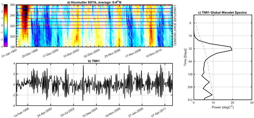
It should be pointed out that choosing different numbers and locations of base points (such 4, 6 or 10) and shifting them together in the zonal direction within the TIW active region give similar results. To capture TIWs westward propagation and thus the main TIW period, we define TIW₂ in the same way as TIW₁, except the base points are all shifted by a fixed distance representing a 90° degree zonal phase shift (i.e. roughly 6.25° in longitude). (2) $$TI{W}_2(t)=\sum \pm \mathit{SST}\prime (t,\mathit{nodes}+{6.25}^{\circ })$$(2)

Thus, the TIWs propagation characteristics (amplitude and phase) are contained in the quantity Z: (3) $$Z=TI{W}_1+\mathit{iTI}{W}_2$$(3) and the TIW amplitude is simply: (4) $$\left|Z\right|=TI{W}_{12}=\sqrt{TI{W}_1^2+TI{W}_2^2}$$(4)

This way of quantifying TIWs is original, yet extremely simple compared to prior methods. Historically, complex EOF (Lyman et al. 2007) or demodulation (Kutsuwada and McPhaden 2002) were commonly used to characterise TIWs and in general any propagating features for these methods allows evaluating both an amplitude and a phase information. Our approach doesn’t involve any mathematical transformation beforehand, is time independent and could, for instance, easily be implemented routinely to evaluate and/or parameterise TIWs in coarse-resolution models (i.e. which does not explicitely resolve them).

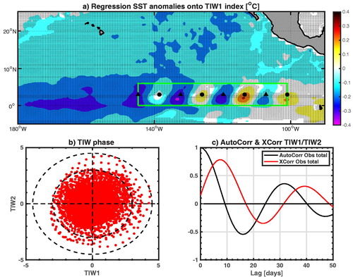
Figure 1a shows the time-longitude Hovmöller diagram of daily SST anomalies used to obtain such TIWs indices zoomed over the period 1997–2011. The corresponding extracted TIW₁ index is shown on Fig. 1b and its global wavelet spectrum on Fig. 1c. The TIW phase diagram is shown in Fig. 2b and exhibits a regular wave propagation pattern. The regression of daily SST anomalies onto TIW₁ shown in Fig. 2a displays the typical equatorial TIWs cusps at the right locations as compared with the spatial pattern of the daily SSTA’s 6^th mode of the Emprirical Orthogonal Functions decomposition, which accounts for TIW variability (Supplementary material Fig. S1a). This confirms the ability of our indices to capture both TIW propagation (i.e. phase and amplitude) and spatial structure. The TIW spectra obtained from both the direct TIW₁ index and the principal component from the EOF decomposition exhibit a significant energy in a broad 20–40 days band as noted by previous studies (Figs. 1c and S1c). A preliminary visual inspection of TIW₁ timeseries also reveals a strong annual and interannual modulation of its enveloppe (i.e. TIWs activity/amplitude, cf. Fig. 2b). The TIW₂ index is nearly a 9-day phase shift of TIW₁ and has similar spatio-temporal and spectral features (e.g. propagation, amplitude… Not shown).

3. A linear model with a time-varying damping rate for TIW amplitude

3.1. Model description and parameters

A stochastically-forced model of climate variability, in which slow changes of climate (i.e. low frequency modulation) are explained as the integral response to continuous white noise forcing, has first been introduced by Hasselmann (1976) and Frankignoul and Hasselmann (1977). It can be written as follows: $\frac{dZ}{dt}=-m(t)Z+\omega (t)$, where Z is the climate variable, ω the white noise forcing and m, the resistance of Z to changes produced by the forcing). Starting from the observation that most climate variables vary seasonally, de Elvira and Lemke (1982) extended this original stochastic climate model by including an annual feedback in m(t). For instance, Stuecker et al. (2017) used this extended model to study the variability of the Indian Ocean Dipole. In their formulation, $m(t)=-{\lambda }_0+{\lambda }_A\hspace{0.17em}\text{cos}\hspace{0.17em}({\omega }_a(t)+\varphi )$, where λ₀ is the mean SST damping rate, λ_A the SST damping rate annual cycle and ϕ its phase. Here, we test the hypothesis that the modulation of TIW amplitude is not only a response of the tropical Eastern Pacific annual cycle but also of ENSO and possibly of the nonlinear interaction between these two modes, therefore implying potential rectifying effects of TIWs low-frequency variability onto both ENSO and the annual cycle. The hypothesis of TIWs amplitude modulation being partly driven by a nonlinear interaction between these two modes originates from the observed strong seasonal modulation of TIWs amplitude variance (cf. Fig. 3). Similarly to ENSO synchronisation to the annual cycle, which manifests in the tendency of ENSO events to peak during boreal winter (Stein et al. 2014), both TIW amplitude (Fig. 3a, black line) and TIW amplitude’s variance (Fig. 3b, black line) exhibit a maximum during the boreal summer/fall. Therefore, our postulate is that TIWs amplitude is the result of a stochastically-forced wave with a seasonally and interannually varying damping rate. As an extension of de Elvira and Lemke (1982) and Stuecker et al. (2017), we add an interannually varying damping rate and formulate our model as follows: (5) $$\begin{array}{c}Z=TI{W}_1+\mathit{iTI}{W}_2\\ \frac{dZ}{dt}=\left[-\left({\gamma }_0+\frac{2i\pi }{T}\right)+\left({\gamma }_A\hspace{0.17em}\text{cos}\hspace{0.17em}\frac{2\pi (t-\varphi )}{T_A}\right)+\left({\gamma }_{N}N\mathit{ino}3(t)\right)\right]Z+\omega (t)\\ \hspace{1em}\hspace{1em}\hspace{1em}\hspace{1em}\hspace{1em}\hspace{1em}\hspace{1em}\hspace{1em}\hspace{1em}\hspace{1em}\hspace{1em}\downarrow \hspace{1em}\hspace{1em}\hspace{1em}\hspace{1em}\hspace{1em}\hspace{1em}\hspace{1em}\hspace{1em}\hspace{1em}\hspace{1em}\hspace{1em}\hspace{1em}\hspace{1em}\hspace{1em}\hspace{1em}\hspace{1em}\hspace{1em}\hspace{1em}\downarrow \hspace{1em}\hspace{1em}\hspace{1em}\hspace{1em}\hspace{1em}\hspace{1em}\hspace{1em}\hspace{1em}\hspace{1em}\hspace{1em}\hspace{1em}\hspace{1em}\hspace{1em}\hspace{1em}\hspace{1em}\hspace{1em}\downarrow \hspace{1em}\hspace{1em}\hspace{1em}\hspace{1em}\hspace{1em}\hspace{1em}\hspace{1em}\hspace{1em}\hspace{1em}\hspace{1em}\hspace{1em}\downarrow \\ \mathrm{\hspace{1em}\hspace{1em}}\mathit{TIW}\mathit{oscillator}\hspace{1em}\hspace{1em}\hspace{1em}\hspace{1em}\hspace{1em}\hspace{1em}\hspace{1em}\hspace{1em}\mathit{TIW}\times AC\hspace{1em}\hspace{1em}\hspace{1em}\hspace{1em}\hspace{1em}\hspace{1em}\mathit{TIW}\times \mathit{ENSO}\hspace{1em}\hspace{1em}\hspace{1em}\mathit{Noise}\end{array}$$(5) where dZ/dt is the TIW amplitude tendency, ω(t) is a white noise forcing and Nino3(t) the interannual (ENSO) forcing. The strength of the noise impacts the amplitude of the solution but has no effect on its spectral properties. The primary objective of the present study is to assess TIWs amplitude’s variability, thus in the following we will only present standardised daily time series. Two daily ENSO forcings of different complexity are tested: (i) the classic Niño3 index (SST anomalies averaged in the Eastern Pacific box 90°W-150°W; 5°S-5°N), (ii) an ideal ENSO forcing, i.e. a simple sinusoidal interannual oscillation, $\mathit{Nino}3(t)=\hspace{0.17em}\text{cos}\hspace{0.17em}\frac{2\pi (t-{\varphi }_2)}{T_E}$ with T_E = 1100 days, i.e. the ENSO main period (cf. Niño3 spectrum, i.e. red line on Supplementary material Fig. S2a) and ϕ₂ the phase for the interannual damping rate. T = 36 days and T_A = 365 days are respectively the TIW and annual cycle (AC) periods. Although TIWs cover a wide range of periods (roughly between 15 and 40 days, cf. Fig. 1c, S1c and Lyman et al. 2007), we chose to restrict the characterisation of this phenomenon to its dominant period (i.e. 36 days) as identified on the TIW₁ spectrum (cf. Fig. 1c). γ₀, γ_A and γ_N are respectively the TIWs mean, annual and interannual damping rates. ϕ is the phase for the annual damping rate and is chosen so that TIWs amplitude reaches a maximum in August/September and a minimum in March/April (ϕ=120 days). Based on the TIWs indices auto and cross correlations (Fig. 2c), we estimate a mean TIW damping rate γ₀ of 1/23 days⁻¹.

Fig. 2. (a) Regression of daily SST anomalies onto TIW₁ index (1997–2015). Dots denote the 95% statistical significance level. Black filled triangles and circles show the positions of longitudinal nodes (positive for circles, i.e. red lines on Fig. 1a, and negative for triangles, i.e. blue lines on Fig. 1a). The bottom right panel (b) is the (TIW₁, TIW₂) phase diagram. (c) Auto correlation of TIW₁-TIW₂ in black and cross correlation between TIW₁ and TIW₂ in red.

Several options are available to estimate the model’s parameters. First of all, since our model’s fornulation is similar to a Linear Inverse Model (for a general description, see Penland and Matrosova (1994); Penland and Sardeshmukh (1995) and references therein), we could simply perform a multiple linear regression of TIW amplitude onto the Eastern Pacific SST seasonal cycle and the Niño3 index. This would lead to the estimation of the model’s optimal parameters. However, one can argue that this “tuning method” is too specific to the data and time period considered and leads to an artificially too optimised solution. In order to stay as general as possible, and in a similar fashion as for γ₀, we choose to estimate γ_A and γ_N only from the decorrelation time of observed TIWs. To do so we contrast auto correlations of (TIW₁-TIW₂) and cross correlations between TIW₁ and TIW₂ to evaluate the TIWs propagation e-folding times (or growth rates) during different seasons of climatological years (for γ_A) and different phases of ENSO (for γ_N) respectively. We distinguish between El Niño, La Niña and climatological (or neutral) years following the NOAA Climate Prediction Center classification. ENSO seasons are from November to February and 1997/98, 2002/03, 2006/07, 2009/10, 2015/16 are considered El Niño events; while 1998/99, 1999/2000, 2000/01, 2007/08, 2010/11, 2011/12 are considered La Niña events. 1997/98, 2009/10 and 2015/16 are considered intense El Niño events. 1998/99, 1999/2000 and 2007/08 are considered intense La Niña events. 2001/02, 2004/05, 2005/06, 2008/09, 2012/13, 2013/14 and 2014/15 are classified as climatologial calendar years (i.e. neutreal ENSO conditions). The estimations of these different TIWs growth rates are presented in Fig. 4a and c and show, as expected, a longer persistance of TIWs activity in summer/fall and during La Niña than in winter/spring (Fig. 4a) and during El Niño (Fig. 4c). Following the notations introduced in Fig. 4b and d, we estimate γ_A and γ_N as follows:

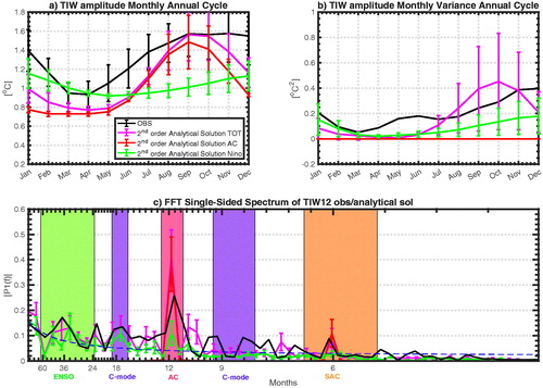
Fig. 3. (a) Annual cycle (monthly mean climatology) of the observed TIW amplitude (1997-2015) (black) and of the ensemble average of the 2^nd order TIW amplitude analytical solution inferred with different reasonable values of γ_A/γ₀ and γ_N/γ₀ ($0.2\le \left|\frac{{\gamma }_A}{{\gamma }_0}\right|,\left|\frac{{\gamma }_N}{{\gamma }_0}\right|\le 0.8$ ) and different versions of the model, i.e. using only a annually-varying TIW damping rate (TIWxAC) in red, using only an interannually-varying TIW damping rate (TIWxNino) in green and using both (TIWxTOT) in magenta. (b) Same but for the monthly variance of TIW amplitude. (c) FFT single-sided spectrum of the observed TIW amplitude (i.e. |Z| = TIW₁₂, black) and ensemble averaged of FFT single-sided amplitude spectra of the 2^nd order approximation of the TIW amplitude analytical solution for the different versions of the model (same colour code as (a)). The dashed blue line indicates the averaged spectrum of 5000 generations of a random red noise process. The Coloured vertical bands indicate select time scales: ENSO (2.5-5 years) in green, the Annual Cycle (AC, 340-390 days) in pink, the Semi Annual Cycle (SAC, 160-200 days) in orange, and the combination mode (C-MODE) in purple. Period: Jan 1^st 1997-Dec 31^st 2015.

${\gamma }_A=\frac{\delta {\gamma }_A}{2}\frac{\delta T_A}{\delta T_{\mathit{TOT}}}\mathrm{and}{\gamma }_N=\frac{\delta {\gamma }_N}{2}\frac{\delta T_N}{\delta T_{\mathit{TOT}}};$ δT_TOT is the maximum amplitude of the total SST signal (climatology plus interannual anomalies), i.e. δT_TOT = max(δT_A+δT_N) over the total time period. Based on this evaluation, we estimate the following rounded parameters: γ_A/γ₀ = 0.30 and γ_N/γ₀ = −0.50. Interestingly, while the TIWs seasonal growth rate changes rather linearly with the climatological equatorial SST (and SST meridional gradient, cf. Fig. 4b), the TIWs interannual growth rate exhibits a strong nonlinear relationship with the SST interannual anomalies (Fig. 4d). The nonlinear relationship between the interannual TIW growth rate and equatorial SST anomalies is best represented by a 3^rd order polynom, which accounts for the asymmetrical nature of this nonlinearity (i.e. the ENSO asymmetrical feedback on TIW amplitude; An (2008)). To include this nonlinear effect, a more refined version of the model is adopted hereafter; and instead of Equation (5)(5) $$\begin{array}{c}Z=TI{W}_1+\mathit{iTI}{W}_2\\ \frac{dZ}{dt}=\left[-\left({\gamma }_0+\frac{2i\pi }{T}\right)+\left({\gamma }_A\hspace{0.17em}\text{cos}\hspace{0.17em}\frac{2\pi (t-\varphi )}{T_A}\right)+\left({\gamma }_{N}N\mathit{ino}3(t)\right)\right]Z+\omega (t)\\ \hspace{1em}\hspace{1em}\hspace{1em}\hspace{1em}\hspace{1em}\hspace{1em}\hspace{1em}\hspace{1em}\hspace{1em}\hspace{1em}\hspace{1em}\downarrow \hspace{1em}\hspace{1em}\hspace{1em}\hspace{1em}\hspace{1em}\hspace{1em}\hspace{1em}\hspace{1em}\hspace{1em}\hspace{1em}\hspace{1em}\hspace{1em}\hspace{1em}\hspace{1em}\hspace{1em}\hspace{1em}\hspace{1em}\hspace{1em}\downarrow \hspace{1em}\hspace{1em}\hspace{1em}\hspace{1em}\hspace{1em}\hspace{1em}\hspace{1em}\hspace{1em}\hspace{1em}\hspace{1em}\hspace{1em}\hspace{1em}\hspace{1em}\hspace{1em}\hspace{1em}\hspace{1em}\downarrow \hspace{1em}\hspace{1em}\hspace{1em}\hspace{1em}\hspace{1em}\hspace{1em}\hspace{1em}\hspace{1em}\hspace{1em}\hspace{1em}\hspace{1em}\downarrow \\ \mathrm{\hspace{1em}\hspace{1em}}\mathit{TIW}\mathit{oscillator}\hspace{1em}\hspace{1em}\hspace{1em}\hspace{1em}\hspace{1em}\hspace{1em}\hspace{1em}\hspace{1em}\mathit{TIW}\times AC\hspace{1em}\hspace{1em}\hspace{1em}\hspace{1em}\hspace{1em}\hspace{1em}\mathit{TIW}\times \mathit{ENSO}\hspace{1em}\hspace{1em}\hspace{1em}\mathit{Noise}\end{array}$$(5) , we use the following: (6) $$\frac{dZ}{dt}=[-\left({\gamma }_0+\frac{2i\pi }{T}\right)+\left({\gamma }_A\hspace{0.17em}\text{cos}\hspace{0.17em}\frac{2\pi (t-\varphi )}{T_A}\right)+\left({\gamma }_{N}N\mathit{ino}3(t)\right)+\left({\gamma }_{N^3}N\mathit{ino}3{(t)}^3\right)]Z+\omega (t)$$(6)

Using a 3^rd-order polynomial fit, in the least square sense, we estimate ${\gamma }_{N^3}=0.007$. It is worth noting that, while this effect might slightly enhance the asymmetry of TIWs activity between the ENSO phases, it will not be its main contributor. The TIWs activity’s asymmetry will mostly emerge from the interannually varying TIWs growth rate’s term (γ_NNino3(t) in Eq. 6(6) $$\frac{dZ}{dt}=[-\left({\gamma }_0+\frac{2i\pi }{T}\right)+\left({\gamma }_A\hspace{0.17em}\text{cos}\hspace{0.17em}\frac{2\pi (t-\varphi )}{T_A}\right)+\left({\gamma }_{N}N\mathit{ino}3(t)\right)+\left({\gamma }_{N^3}N\mathit{ino}3{(t)}^3\right)]Z+\omega (t)$$(6) ).

3.2. Approximation of the TIW amplitude’s analytical solution and parameters sensitivity

As long as |γ_A/γ₀| < 1, |γ_N/γ₀| < 1 and |γ_N³/γ₀| < 1, the oscillating solutions Z stay in a stable damped regime and we can use a second order Taylor series expansion (O(ε²)) to approximate the analytical solution of TIWs amplitude |Z|. After some mathematical steps detailed in the appendix A, it can be shown that the low-frequency modulation of TIWs amplitude has the following form: (7) $$〈\left|Z^2\right|〉=K{e}^{-{\gamma }_0}\left[1+\frac{m(t)}{{\gamma }_0}+\frac{m^2(t)}{{\gamma }_0^2}\right]$$(7) where $〈\left|Z^2\right|〉$ represents the slow variation of TIWs amplitude |Z|² (i.e. the low-frequency modulation, diagnosed in the following as the 50-days running mean of the solution Z²) and $m(t)=({\gamma }_A\hspace{0.17em}\text{cos}\hspace{0.17em}\frac{2\pi (t-\varphi )}{T_A})+({\gamma }_{N}N\mathit{ino}3(t))+({\gamma }_{N^3}N\mathit{ino}3{(t)}^3)$

The 2^nd order approximation of our simple model’s solution exhibits similar spectral properties as the observed TIW amplitude (cf. Fig. 3c black and magenta lines). In particular, this model is able to produce the variability associated with the combination mode (C-MODE) between the annual cycle and ENSO. This variability originates from the nonlinear interaction between ENSO and the annual cycle found within the m²(t) term of the analytical solution: (8) $$C-\mathit{MODE}=\frac{2}{{\gamma }_0}\times \left({\gamma }_A\hspace{0.17em}\text{cos}\hspace{0.17em}\frac{2\pi (t-\varphi )}{T_A}\right)\times \left({\gamma }_{N}N\mathit{ino}3(t)\right)$$(8)

As explained in Section 1, this combination tone mostly manifests itself at a couple frequencies f_C-MODE = f_AC ± f_ENSO (Fig. 3c, frequency bands highlighted in purple) and cannot be explained by any direct external forcing (Stuecker et al. 2013; 2017).

Additionally, we performed a parameter sensivity analysis presented in Supplementary material Fig. S3 (cf. supplemental material). It shows the sensitivity of some features of TIW amplitude’s analytical solution to the |γ_A/γ₀| and |γ_N/γ₀| ratio values. This not only corroborates the parameters estimation presented in the previous section based on a physical analysis of the observed TIWs features (and not from an optimal tuning method through linear regressions), but also illustrates the robustness of our model and its analytical solution within the parameters domain.

3.3. Sensitivity of numerical and analytical solutions to forcing

Now that the TIW model can reproduce realistically the main spectral and temporal features of the observed TIW amplitude variability, we explore the sensitivity of the analytical and numerical solutions to different forcing terms. To do so, we compare the spectral and temporal properties of the TIW amplitude variability generated by a 50-members ensemble of three different versions of the linear model: the full model forced by both the annually and interannually TIW varying damping rates (noted TIWxTOT, i.e. all terms included, γ_N ≠ 0, γ_A ≠ 0 and γ_N³ ≠ 0), the model forced only by the annually varying TIW damping rate (noted TIWxAC, i.e. γ_N = 0 and γ_N³ = 0) and the model forced only by the interannually varying TIW damping rate (noted TIWxNino, i.e. γ_A = 0). All versions of the model are integrated from January 1^st 1997 to August 31^st 2016 using a 4^th order Runge-Kutta method and the parameters values from Section 3.1.

Fig. 4. (a) Average of (TIW₁-TIW₂) autocorrelations (in black) and (TIW₁,TIW₂) cross correlations (in red) logarithm for climatological years (i.e. neither El Niño nor La Niña years) between November and February. The black dotted line represents the best linear fit to these curves local maxima or in other words the estimation of TIWs propagation e-folding time during neutral years. Similarly, the green (magenta) dotted line represents the best linear estimation of TIWs propagation e-folding time for El Niño (La Niña) years. The red (blue) dotted line represents the best linear estimation of TIWs propagation e-folding time for extreme El Niño (La Niña) years. (b) The inverse of these e-folding times (in other words, TIWs growth rates) are represented as a function of the daily equatorial (2°S-4°N; 180°W-100°W) SST anomalies averaged during the corresponding periods and years (in red). The black curve is the same but for TIWs growth rates as a function of the meridional gradient of SST anomalies, i.e. the difference between the equatorial region average and the [7°N-13°N; 180°W-100°W] average. (c) Same as (a) but during different seasons of neutral years: Auto (black) and cross (red) correlations logarithm averaged during February-September. The corresponding e-folding time linear estimation is shown in the dotted black line. The green, respectively magenta, dotted line represents the best linear estimation of TIWs propagation e-folding time during the summer and fall (July-September), respectively spring and winter (February-April) of neutral years. (d) Same as (b) but the TIWs seasonal growth rates are shown as a function of the corresponding equatorial SST average in red and the meridional climatological SST gradient in black.

Figure 5a shows the timeseries of the observed (black line) and simulated TIW amplitude (blue line for the ensemble average and thin Coloured lines for all individual members integrated using the TIWxTOT version) along with the 2^nd order approximation of the analytical solution (red line). The full model (TIWxTOT i.e. γ_N ≠ 0, γ_A ≠ 0 and γ_N³ ≠ 0) simulates realistically the TIW amplitude variability, as demonstrated by a good correlation between the observed and the analytical solution, respectively ensemble averaged, TIW amplitude (r = 0.72, respectively 0.75; cf Fig. 5a). Figure 5b (respectively Fig. 6a) summarises the spectral properties of the analytical solution (respectively ensemble-averaged solutions) of the TIW amplitude simulated by different forcing experiments of the linear model. Additionally, Fig. 3c presents the analytical solutions power spectra from different versions of the model (i.e. TIWxTOT, TIWxAC and TIWxNino) and for a wide range of parameters values (i.e. $0.2\le \left|\frac{{\gamma }_A}{{\gamma }_0}\right|,\left|\frac{{\gamma }_N}{{\gamma }_0}\right|\le 0.8$). The TIW amplitude generated by the fully forced version of the model exhibits a relatively similar spectrum (magenta line) as the one from the observed TIW amplitude (thick black line), significant in particular for the key annual, ENSO and C-MODE frequencies. Interestingly, we note the presence of a significant peak of near decadal variability around 7–10 years⁻¹ in the spectrum of both the observed and simulated TIW amplitude (as well as in the spectrum of Niño3 index, cf. red line in Supplementary material Fig. S1a). However, although barely significant as compared to a random red noise process, this frequency peak is stronger in the spectrum of the TIW amplitude generated by the full forcing experiment (TIWxTOT) and less energetic in the ENSO-only case (see comparison between green and magenta spectra in Figs. 3c, 5b and 6a). This suggests that this near-decadal TIW amplitude variability might be amplified by rectification processes emerging from the nonlinear interaction between the annual cycle, ENSO and the seasonal and interannual modulations of TIW amplitude.

The asymmetric feedback between the ENSO state and TIW amplitude first evidenced by An (2008) is also captured by this simple model with an enhanced, respectively suppressed TIW amplitude during La Niña, respectively El Niño, as shown in Fig. 6c. Interestingly, this simple model also seems to capture the nonlinear interaction between the Eastern Pacific annual cycle and TIWs amplitude’s annual modulation, as shown in Fig. 6b by a shift in phase of ≈40 days and a broadening from the analytical solution to the forcing’s seasonal cycle. This indicates a potential nonlinear rectification of the tropical Eastern Pacific upper-ocean seasonal heat budget by the modulation of TIWs amplitude.

As evidenced on Supplementary material Fig. S2a (red line), the direct ENSO forcing displays a significant peak of variability in the C-MODE frequency band. Therefore, there is a chance that the C-MODE peak in the simulated TIW amplitude emerges from this prescribed ENSO forcing rather than from the nonlinear combination between the ENSO and annual frequencies. The use of interannual forcing of different complexity and in particular the comparison between TIW amplitude solutions inferred from an ideal (i.e. purely sinusoidal by construction and thus containing no C-MODE variability) and the prescribed ENSO forcing confirm that most of the C-MODE variability emerges from the nonlinear interaction between the Annual Cycle and ENSO (cf. Figs. 3c and 6a as compared to Supplementary material Fig. S4c which shows the spectra of the different versions of the model integrated using an ideal ENSO forcing).

Additionally, Supplementary material Fig. S2b shows the spectrum of the observed and simulated TIW, i.e. the TIW₁ index (real part of Z in the nonlinear model). The richness in TIW spectrum (20–40 days⁻¹) only emerges when both the annually and inter-annually varying TIW damping rates are included in the model and cannot be accounted for without the nonlinear interaction between the Eastern Pacific Annual Cycle and ENSO. Although beyond the scope of this paper, the complex variability of the TIW high-frequency process arises partly from nonlinear dynamics in the Eastern Pacific. TIW amplitude modulation can potentially influence the local SST variability at different timescales, which in turn can alter the typical patterns of the annual and interannual atmospheric variability in this key region where sits the Inter-Tropical Convergence Zone.

4. Conclusion and discussion

In this paper, we developed a simple TIWs stochastic linear model forced by ENSO and the annual cycle to assess the deterministic low frequency modulation of TIWs variance. In particular, we study the effect of the Cold Tongue SST annual cycle and ENSO on the modulation of TIW activity. Both the analytical and numerical solutions of our simple model depict realistically the basic features of TIWs amplitude variability; namely the seasonal increase in TIWs variance during summers and falls and the nonlinear relationship with the ENSO phase characterised by a suppression, respectively increase of TIW activity during El Niño, respectively La Niña. The novelty result evidenced through this innovative framework is that a significant fraction (diagnosed by a significant spectral peak in the C-MODE frequency band as compared to a red noise process) of TIWs amplitude modulation emerges from the deterministic nonlinear interaction between ENSO and the annual cycle and is therefore predictable. This reflects a similar combination mode dynamic as the one described by Stuecker et al. (2013; 2017) but with a different seasonality (enhanced interaction during the northern hemisphere summer/fall). Therefore, this study revealed a new ENSO combination mode and a new route of ENSO frequency cascade through both the oceanic and atmospheric responses to TIW-induced changes in the upper-ocean heat transport. The deterministic variability of this state-dependent oceanic stochastic forcing will potentially trigger different oceanic and atmospheric teleconnections in the tropical climate system and deserves more in-depth investigation.

Additionally, the observed interannual anomalies of the 50-days running TIW amplitude are significantly correlated with those from the model’s 50-member ensemble average (not shown) and the analytical solution (Fig. 7a). Moreover, this variability is negatively correlated with ENSO. Since, in our simple TIW model, ENSO modulates TIW activity, it can be easily proved that the interannual anomalies of TIW variance will induce a proportional and significant variation in TIW-induced nonlinear dynamic heating (NDH) owing to the strong TIW heat transport meridional convergence -∇·(v′T′) (mainly due to the strong SST meridional gradient). This will be the object of an upcoming article but preliminary results reveal a high correlation between the TIWs-induced nonlinear meridional heat flux (-v’T’) and the interannual anomalies of both the observed (r = 0.57) and theoretical (r = 0.78) TIW amplitude (not shown). Thus, our simple model provides a simple analytical theory to describe the asymmetric feedback between the ENSO state and TIW activity, which was first empirically introduced by An (2008) into a simple ENSO model to assess the TIW contribution to the observed El Niño/La Niña asymmetry. We can now give an analytical formulation for the ENSO-induced TIW NDH feedback onto ENSO as follows: (9) $$ND{H}_{\mathit{TIW}}\approx -\nabla .(v\prime T\prime )\approx \left(2\frac{{\gamma }_A{\gamma }_N}{{\gamma }_0^2}\text{cos}\hspace{0.17em}\left(\frac{2\pi (t-\varphi )}{T_A}\right)\times \mathit{Nino}3(t)\right)+{\left(\frac{{\gamma }_N}{{\gamma }_0}\right)}^{2}N\mathit{ino}3{(t)}^2+{\left(\frac{{\gamma }_{N^3}}{{\gamma }_0}\right)}^{2}N\mathit{ino}3{(t)}^6+\left(2\frac{{\gamma }_A{\gamma }_{N^3}}{{\gamma }_0^2}\text{cos}\hspace{0.17em}\left(\frac{2\pi (t-\varphi )}{T_A}\right)\times \mathit{Nino}3{(t)}^3\right)+2\frac{{\gamma }_A{\gamma }_{N^3}}{{\gamma }_0^2}N\mathit{ino}3{(t)}^4$$(9)

Fig. 5. (a) Individual members (thin Coloured lines) and ensemble average (thick blue line) of the daily TIW amplitude numerical solutions using the full TIWxTOT version of the model. The black line shows the observed daily TIW amplitude. The thick red line is the 2^nd order analytical solution of TIW amplitude. All time series are normalised and smoothed using a 50-days running mean. (b) Spectra of the observed and 2^nd order approximation of the analytical solution of TIW amplitude from different sensitivity experiments. Thick black lines for observation, red for the experiments using only a annually-varying TIW damping rate (TIWxAC), green for the experiments using only an interannually-varying TIW damping rate (TIWxNino) and magenta for the experiments using both (TIWxTOT). The dashed blue line indicates the averaged spectrum of 5000 generations of a random red noise process.

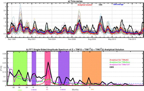
Fig. 6. (a) Spectra of the observed and ensemble average of TIW amplitude (Z = TIW12) simulated by different sensitivity experiments (the Coloured bands representing different typical timescales, see Fig. 5b caption). Thick black lines for observation, red for the experiments using only a annually-varying TIW damping rate (TIWxAC), green for the experiments using only an interannually-varying TIW damping rate (TIWxNino) and magenta for the experiments using both (TIWxTOT). The dashed blue line indicates the averaged spectrum of 5000 generations of a random red noise process. (b) Annual cycle of the observed (black line), the ensemble average (blue line) and the analytical solution (red) of TIW amplitude; the annual cycle of the model forcing is shown in green. (c) Scatter plot of simulated TIW amplitude (TIWxTOT ensemble average) versus the prescribed Niño3 forcing.

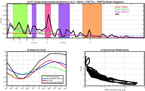
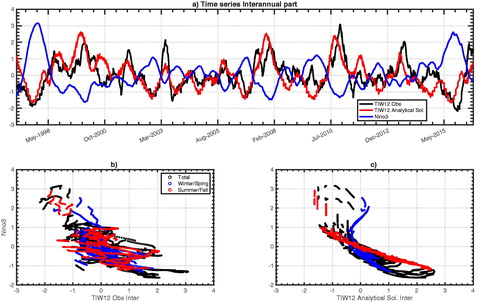
Fig. 7. (a) Observed interannual part (i.e. cleared from the 1997–2015 monthly mean climatology) of TIW amplitude (black) and interannual part of the analytical solution 2^nd order approximation of TIW amplitude (red) using the following set of parameters: γ₀ = 1/23 days⁻¹_; γ_A/γ₀ = 0.3; γ_N/γ₀ = −0.5 and γ_N³ = 0.007; The correlation between these two timeseries is 0.65. The blue line shows the Niño3 index. (b) Scatter plot of the nonlinear relationship between the observed interannual TIW amplitude and ENSO (Niño3 index); Red (summer/fall only) and blue (winter/spring only) dots highlight the seasonality of this relationship. (c) Same as (b) for the the nonlinear relationship between the 2^nd order approximation of the analytical solution of the interannual TIW amplitude and ENSO.

This formulation not only accounts for the response to the ENSO-Annual Cycle interaction but also for potentially significant higher order nonlinear interactions, i.e. following the notation introduced in Section 1, at frequencies 2f, 4f, 6f and 1 ± 3f. Despite the fact that our model is linear, this approximate analytical solution, obtained by a perturbation method, demonstrates clearly that the TIW feedback onto ENSO is not only nonlinear but also strongly modulated by the seasonal cycle (cf. Fig. 7b and c). This nonlinearity comes from that fact that this feedback operates through the TIW nonlinear heat transport convergence -∇·(v′T′), i.e. NDH processes. We plan to conduct further investigations motivated by this conceptual advancement, to assess the interactions between ENSO and TIW activity.

Furthermore, the simple theoretical framework presented here can be generalised to assess the modulation by the annual cycle, ENSO and their combined effect of any so-called state-dependent transients of the tropical climate system. A stochastically forced linear model of high frequency processes with periods much shorter than ENSO, with an annually and interannually varying damping rate, provides a good approximate to infer nonlinear deterministic rectifications through the covariance fields. A follow-up application of this new framework is the study of the deterministic modulation of MJO/WWB activity due to ENSO, the annual cycle and their nonlinear combination. This will be the topic of an oncoming research article.

Supplemental data

Supplemental data for this article can be accessed here.

Additional information

Funding

This project was supported by the U.S. National Science Foundation grant ATM1406601 and the French Agence Nationale de la Recherche project MOPGA “Trocodyn”, grant number ANR-17-MPGA-0018.

Appendix A

Approximation of the analytical solution of the low frequency amplitude modulation of TIWs using a Taylor series expansion:

-To stay in a stable damped regime, let $\left|\frac{{\gamma }_A}{{\gamma }_0},\frac{{\gamma }_N}{{\gamma }_0},\frac{{\gamma }_{N^3}}{{\gamma }_0}\right|<(1,1,1)$

and $m(t)=({\gamma }_A\hspace{0.17em}\text{cos}\hspace{0.17em}\frac{2\pi (t-\varphi )}{T_A})+({\gamma }_{N}N\mathit{ino}3(t))+({\gamma }_{N^3}N\mathit{ino}3{(t)}^3)$

0 -order solution: (i) $$\frac{d{Z}_0}{dt}=\left[-\left({\gamma }_0+\frac{2i\pi }{T}\right)\right]Z_0+\omega (t)\hspace{1em}$$(i)

1^st-order solution: (ii) $$\frac{d{Z}_1}{dt}=\left[-\left({\gamma }_0+\frac{2i\pi }{T}\right)\right]Z_1+m(t)Z_0\hspace{1em}$$(ii)

2^nd-order solution: (iii) $$\frac{d{Z}_2}{dt}=\left[-\left({\gamma }_0+\frac{2i\pi }{T}\right)\right]Z_2+m(t)Z_1+m^2(t)Z_0^2\hspace{1em}$$(iii)

…

Total Solution: $Z={\sum }_i{Z}_i{\left|Z\right|}^2={\sum }_i{Z}_i{\sum }_i{Z}_i^{*}$

2nd order approximation: $$-\forall (i,j)\left|\right(i+j)>2,\hspace{1em}{Z}_i{Z}_j^{*}=0\mathit{and}\frac{d{Z}_i{Z}_j^{*}}{dt}=0$$ (A) $$\begin{array}{c}{\left|Z\right|}^2=\left(Z_0+Z_1+Z_2\right)\left(Z_0^{*}+Z_1^{*}+Z_2^{*}\right)\\ {\left|Z\right|}^2={\left|Z_0\right|}^2+{\left|Z_1\right|}^2+\left(Z_1{Z}_0^{*}+Z_0{Z}_1^{*}\right)+\left(Z_2{Z}_0^{*}+Z_0{Z}_2^{*}\right)\end{array}$$(A) a/Step 1:

- From (i) (A1) $$Z_0^{*}\frac{d{Z}_0}{dt}=\left[-\left({\gamma }_0+\frac{2i\pi }{T}\right)\right]{\left|Z_0\right|}^2+Z_0^{*}\omega (t)$$(A1) (A2) $$Z_0\frac{d{Z}_0^{*}}{dt}=\left[-\left({\gamma }_0-\frac{2i\pi }{T}\right)\right]{\left|Z_0\right|}^2+Z_0{\omega }^{*}(t)$$(A2)

- Eqs. (A1)+(A2): $$\frac{d{\left|Z_0\right|}^2}{dt}=-2{\gamma }_0{\left|Z_0\right|}^2+Z_0^{*}\omega (t)+Z_0{\omega }^{*}(t)$$

- Let $〈X〉$ represents the slow variation of X (B) $${〈(A3)〉}_{\mathbf{\to }}〈{\left|Z_0\right|}^2〉=\frac{〈Z_0^{*}\omega (t)+Z_0{\omega }^{*}(t)〉}{2{\gamma }_0}$$(B)

${\left|T_0\right|}^2$ represents the unmodulated background noise.

b/Step 2:

- From (i) (A4) $$Z_1^{*}\frac{d{Z}_0}{dt}=\left[-\left({\gamma }_0+\frac{2i\pi }{T}\right)\right]Z_0{Z}_1^{*}+Z_1^{*}\omega (t)$$(A4) (A5) $$Z_1\frac{d{Z}_0^{*}}{dt}=\left[-\left({\gamma }_0+\frac{2i\pi }{T}\right)\right]Z_1{Z}_0^{*}+Z_1{\omega }^{*}(t)$$(A5)

- From (ii) (A6) $$Z_0^{*}\frac{d{Z}_1}{dt}=\left[-\left({\gamma }_0+\frac{2i\pi }{T}\right)\right]Z_1{Z}_0^{*}+{\left|Z_0\right|}^2\omega (t)$$(A6) (A7) $$Z_0^{}\frac{d{Z}_1^{*}}{dt}=\left[-\left({\gamma }_0+\frac{2i\pi }{T}\right)\right]Z_0{Z}_1^{*}+{\left|Z_0\right|}^2\omega (t)$$(A7)

- Eqs. (A4)+(A5)+(A6)+(A7): (A8) $$\frac{d{Z}_1{Z}_0^{*}}{dt}+\frac{d{Z}_0{Z}_1^{*}}{dt}=2{\left|Z_0\right|}^{2}m(t)-2{\gamma }_0\left(Z_1{Z}_0^{*}+Z_0{Z}_1^{*}\right)+Z_1^{*}\omega (t)+Z_1{\omega }^{*}(t)$$(A8)

- Since $〈Z_1^{*}\omega (t)+Z_1{\omega }^{*}(t)〉=0$ $$〈(A8)〉$$ (C) $${〈(A8)〉}_{\mathbf{\to }}〈Z_0^{*}{Z}_1+Z_0{Z}_1^{*}〉=\frac{{\left|T_0\right|}^{2}m(t)}{{\gamma }_0}$$(C)

c/Step 3:

- From (ii) (A9) $$Z_1^{*}\frac{d{Z}_1}{dt}=\left[-\left({\gamma }_0+\frac{2i\pi }{T}\right)\right]{\left|Z_1\right|}^2+m(t)Z_1^{*}{Z}_0$$(A9) (A10) $$Z_1\frac{d{Z}_1^{*}}{dt}=\left[-\left({\gamma }_0+\frac{2i\pi }{T}\right)\right]{\left|Z_1\right|}^2+m(t)Z_0^{*}{Z}_1$$(A10)

- Eqs. (A9)+(A10): (A11) $$\frac{d{\left|Z_1\right|}^2}{dt}=-2{\gamma }_0{\left|Z_1\right|}^2+m(t)\left(Z_0^{*}{Z}_1+Z_1^{*}{Z}_0\right)\hspace{1em}$$(A11) (A12) $${〈(11)〉}_{\mathbf{\to }}〈{\left|Z_1\right|}^2〉=\frac{〈Z_0^{*}{Z}_1+Z_1^{*}{Z}_0〉}{2{\gamma }_0}m(t)$$(A12)

- From (A12) and (A8) (D) $$〈|Z_1{|}^2〉=\frac{|Z_0{|}^2{m}^2(t)}{2{\gamma }_0}$$(D)

d/Step 4:

- From (i) (A13) $$Z_2^{*}\frac{d{Z}_0}{dt}=\left[-\left({\gamma }_0+\frac{2i\pi }{T}\right)\right]Z_0{Z}_2^{*}+Z_2^{*}\omega (t)$$(A13) (A14) $$Z_2\frac{d{Z}_0^{*}}{dt}=\left[-\left({\gamma }_0+\frac{2i\pi }{T}\right)\right]Z_2{Z}_0^{*}+Z_2{\omega }^{*}(t)$$(A14)

- From (iii) (A15) $$Z_0^{*}\frac{d{Z}_2}{dt}=\left[-\left({\gamma }_0+\frac{2i\pi }{T}\right)\right]Z_0^{*}{Z}_2+m(t)Z_0^{*}{Z}_1$$(A15) (A16) $$Z_0\frac{d{Z}_2^{*}}{dt}=\left[-\left({\gamma }_0+\frac{2i\pi }{T}\right)\right]Z_2^{*}{Z}_0+m(t)Z_1^{*}{Z}_0$$(A16)

- Eqs. (A13)+(A14)+(A15)+(A16): (A17) $$\frac{d{Z}_2{Z}_0^{*}}{dt}+\frac{d{Z}_0{Z}_2^{*}}{dt}=m(t)\left(Z_1{Z}_0^{*}+Z_0{Z}_1^{*}\right)-2{\gamma }_0\left(Z_2{Z}_0^{*}+Z_0{Z}_2^{*}\right)+Z_2^{*}\omega (t)+Z_2{\omega }^{*}(t)$$(A17)

- Since $〈Z_2^{*}\omega (t)+Z_2{\omega }^{*}(t)〉=0$ (A18) $${〈(A17)〉}_{\mathbf{\to }}〈Z_0^{*}{Z}_2+Z_0{Z}_2^{*}〉=\frac{m(t)}{2{\gamma }_0}〈Z_0^{*}{Z}_1+Z_0{Z}_1^{*}〉$$(A18)

- From (A18) and (C) (E) $$〈Z_0^{*}{Z}_2+Z_0{Z}_2^{*}〉=\frac{{\left|Z_0\right|}^2{m}^2(t)}{2{\gamma }_0^2}$$(E)

Combining (B), (C), (D) and (E) into (A) $$〈{\left|Z\right|}^2〉={\left|Z_0\right|}^2\left[1+\frac{m(t)}{{\gamma }_0}+\frac{m^2(t)}{{\gamma }_0^2}\right]$$ $$〈{\left|Z\right|}^2〉=K{e}^{-{\gamma }_0}\left[1+\frac{m(t)}{{\gamma }_0}+\frac{m^2(t)}{{\gamma }_0^2}\right]$$

References

- Ashok, K., Behera, S. K., Rao, S. A., Weng, H. and Yamagata, T. 2007. El Niño Modoki and its possible teleconnection. J. Geophys. Res 112, C11007. doi:10.1029/2006JC003798
- An, S.-I. 2008. Interannual variations of the tropical ocean in- stability wave and ENSO. J. Climate 21, 3680–3686. doi:10.1175/2008JCLI1701.1
- Battisti, D. S. and Hirst, A. C. 1989. Interannual variability in the tropical atmosphere/ocean system: influence of the basic state and ocean geometry. J. Atmos. Sci. 46, 1687–1712. doi:10.1175/1520-0469(1989)046<1687:IVIATA>2.0.CO;2
- Cane, M. A. and Zebiak, S. E. 1985. A theory for El Niño and the Southern Oscillation. Science 228, 1085–1087. doi:10.1126/science.228.4703.1085
- Capotondi, A., Wittenberg, A. T., Newman, M., Di Lorenzo, E., Yu, J.-Y. and co-authors. 2015. Understanding ENSO diversity. Bull. Amer. Meteor. Soc. 96, 921–938. doi:10.1175/BAMS-D-13-00117.1
- Cox, M. D. 1980. Generation and propagation of 30-day waves in a numerical model of the Pacific. J. Phys. Oceanogr. 10, 1168–1186. doi:10.1175/1520-0485(1980)010<1168:GAPODW>2.0.CO;2
- De Elvira, A. R. and Lemke, P. 1982. A Langevin equation for stochastic climate models with periodic feedback and forcing variance. Tellus 34, 313–320. doi:10.1111/j.2153-3490.1982.tb01821.x
- Düing, W., Hisard, P., Katz, E., Meincke, J., Miller, L. and co-authors. 1975. Meanders and long waves in the equatorial Atlantic. Nature 257, 280–284.,. doi:10.1038/257280a0
- Eisenman, I., Yu, L. and Tziperman, E. 2005. Westerly wind bursts: ENSO’s tail rather than the dog?. J. Climate 18, 5224–5238. doi:10.1175/JCLI3588.1
- Frankignoul, C. and Hasselmann, K. 1977. Stochastic climate models, Part II. Application to sea-surface temperature anomalies and thermocline variability. Tellus 29, 289–305.
- Hansen, D. V. and Paul, C. A. 1984. Genesis and effects of long waves in the equatorial Pacific. J. Geophys. Res. 89, 10431–10440. doi:10.1029/JC089iC06p10431
- Hasselmann, K. 1976. Stochastic climate models Part I. Theory. Tellus 28, 473–485.
- Hendon, H. H., Wheeler, M. and Zhang, C. 2007. Seasonal dependence of the MJO–ENSO relationship. J. Climate 20, 531–543. doi:10.1175/JCLI4003.1
- Im, S.-H., An, S.-I., Lengaigne, M. and Noh, Y. 2012. Seasonality of tropical instability waves and its feedback to the seasonal cycle in the tropical eastern pacific. The Scientific World Journal, 2012, 612048.
- Jiang, N., Neelin, J. D. and Ghil, M. 1995. Quasi-quadrennial and quasi-biennial variability in the equatorial Pacific. Clim. Dyn. 12, 101–112. doi:10.1007/BF00223723
- Jin, F.-F. and Neelin, J. D. 1993. Modes of interannual tropical ocean-atmosphere inter-action—a unified view. Part I: numerical results. J. Atmos. Sci. 50, 3477–3502. doi:10.1175/1520-0469(1993)050<3477:MOITOI>2.0.CO;2
- Jin, F.-F., Neelin, J. D. and Ghil, M. 1994. El Niño on the Devil’s staircase: annual subharmonic steps to chaos. Science 264, 70. doi:10.1126/science.264.5155.70
- Jin, F.-F., Neelin, J. D. and Ghil, M. 1996. El Niño/Southern oscillation and the annual cycle: subharmonic frequency-locking and aperiodicity. Physica D 98, 442–465. doi:10.1016/0167-2789(96)00111-X
- Jin, F.-F. 1997. An equatorial ocean recharge paradigm for ENSO. Part I: conceptual model. J. Atmos. Sci. 54, 811–829. doi:10.1175/1520-0469(1997)054<0811:AEORPF>2.0.CO;2
- Jin, F.-F. 1997. An equatorial ocean recharge paradigm for ENSO. Part II: a striped-down coupled model. J. Atmos. Sci. 54, 830–846. doi:10.1175/1520-0469(1997)054<0830:AEORPF>2.0.CO;2
- Jin, F.-F., Lin, L., Timmermann, A. and Zhao, J. 2007. Ensemble-mean dynamics of the ENSO recharge oscillator under state-dependent stochastic forcing. Geophys. Res. Lett. 34, L0807.
- Kessler, W. S. and Kleeman, R. 2000. Rectification of the Madden-Julian Oscillation into the ENSO cycle. J. Climate 13, 3560–3575. doi:10.1175/1520-0442(2000)013<3560:ROTMJO>2.0.CO;2
- Kleeman, R. and Moore, A. M. 1997. A theory for the limitation of ENSO predictability due to stochastic atmospheric transients. J. Atmos. Sci. 54, 753–767. doi:10.1175/1520-0469(1997)054<0753:ATFTLO>2.0.CO;2
- Kug, J.-S., Jin, F.-F., Sooraj, K. P. and Kang, I.-S. 2008. Evidence of the state-dependent atmospheric noise associated with ENSO. Geophy. Res. Lett. 35, L05701.
- Kug, J.-S., Jin, F.-F. and An, S.-I. 2009. Two-types El Nino: Cold Tongue El Nino and Warm Pool El Nino. J. Climate 22, 1499–1515. doi:10.1175/2008JCLI2624.1
- Kug, J.-S., Sooraj, K. P., Kim, D., Kang, I.-S., Jin, F.-F. and co-authors. 2009. Simulation of state-dependent high-frequency atmospheric variability associated with ENSO. Clim. Dyn. 32, 635–648., doi:10.1007/s00382-008-0434-2
- Kutsuwada, K. and McPhaden, M. J. 2002. Intraseasonal variations in the upper equatorial Pacific Ocean prior to and during the 1997-98 El Niño. J. Phys. Oceanogr. 32, 1133–1149. doi:10.1175/1520-0485(2002)032<1133:IVITUE>2.0.CO;2
- Legeckis, R. 1977. Long waves in the eastern equatorial Pacific Ocean: A view from a geostationary satellite. Science 197, 1179–1181. doi:10.1126/science.197.4309.1179
- Lengaigne, M., Guilyardi, E., Boulanger, J. P., Menkes, C., Delecluse, P. and co-authors. 2004. Triggering of El Niño by westerly wind events in a coupled general circulation model. Clim. Dyn. 23, 601–620., doi:10.1007/s00382-004-0457-2
- Luther, D. S. and Johnson, E. S. 1990. Eddy Energetics in the Upper Equatorial Pacific during the Hawaii-to-Tahiti Shuttle Experiment. J. Phys. Oceanogr. 20, 913–944., doi:10.1175/1520-0485(1990)020<0913:EEITUE>2.0.CO;2
- Lyman, J. M., Johnson, G. C. and Kessler, W. S. 2007. Distinct 17- and 33-day tropical instability waves in subsurface observations. J. Phys. Oceanogr. 37, 855–872. doi:10.1175/JPO3023.1
- McPhaden, M. J., Busalacchi, A. J., Cheney, R., Donguy, J.-R., Gage, K. S. and co-authors. 1998. The tropical ocean-global atmosphere (TOGA) observing system: a decade of progress. J. Geophys. Res. 103, 14169–14240., doi:10.1029/97JC02906
- McPhaden, M. J. 2004. Evolution of the 2002/03 El Niño. Bull. Amer. Meteor. Soc. 85, 677–695. doi:10.1175/BAMS-85-5-677
- Moore, A. M. and Kleeman, R. 1999. Stochastic forcing of ENSO by the intraseasonal oscillation. J. Climate 12, 1199–1220. doi:10.1175/1520-0442(1999)012<1199:SFOEBT>2.0.CO;2
- Neelin, J. D., Battisti, D. S., Hirst, A. C., Jin, F.-F., Wakata, Y. and co-authors. 1998. ENSO theory. J. Geophys. Res. 103, 14261–14290., doi:10.1029/97JC03424
- Penland, C. and Matrosova, L. 1994. A balance condition for stochastic numerical models with application to the El Niño‒Southern oscillation. J. Climate 7, 1352–1372. doi:10.1175/1520-0442(1994)007<1352:ABCFSN>2.0.CO;2
- Penland, C. and Sardeshmukh, P. D. 1995. The optimal growth of tropical sea surface temperature anomalies. J. Climate 8, 1999–2024. doi:10.1175/1520-0442(1995)008<1999:TOGOTS>2.0.CO;2
- Perigaud, C. M. and Cassou, C. 2000. Importance of oceanic decadal trends and westerly wind bursts for forecasting El Niño. Geophys. Res. Lett. 27, 389–392. doi:10.1029/1999GL010781
- Philander, S. G. H. 1978. Instabilities of zonal equatorial currents: Part 2. J. Geophys. Res. 83, 3679–3682. doi:10.1029/JC083iC07p03679
- Philander, S. G. H. and Niño, E. 1990. La Niña, and the Southern Oscillation. Academic Press, San Diego, pp 293.
- Qiao, L. and Weisberg, R. H. 1995. Tropical instability wave kinematics: Observations from the tropical instability wave experiment. J. Geophys. Res. 100, 8677–8693. doi:10.1029/95JC00305
- Reynolds, R. W., Liu, C., Smith, T. M., Chelton, D. B., Schlax, M. G. and co-authors. 2007. Daily high-resolution-blended analyses for sea surface temperature. J. Climate 20, 5473–5496., doi:10.1175/2007JCLI1824.1
- Stein, K., Timmermann, A., Schneider, N., Jin, F.-F. and Stuecker, M. F. 2014. ENSO seasonal synchronization theory. J. Climate 27, 5285–5310. doi:10.1175/JCLI-D-13-00525.1
- Stuecker, M. F., Timmermann, A., Jin, F.-F., McGregor, S. and Ren, H.-L. 2013. A combination mode of the annual cycle and the El Niño/Southern Oscillation. Nature Geosci. 6, 540–544. doi:10.1038/ngeo1826
- Stuecker, M. F., Jin, F.-F. and Timmermann, A. 2015. El Nino-Southern Oscillation frequency cascade.. Proc. Natl. Acad. Sci. USA. 112, 13490–13495. doi:10.1073/pnas.1508622112
- Stuecker, M. F., Timmermann, A., Jin, F.-F., Chikamoto, Y., Zhang, W. and co-authors. 2017. Revisiting ENSO/Indian Ocean Dipole phase relationships. Geophys. Res. Lett. 44, 2481–2492., doi:10.1002/2016GL072308
- Suarez, M. J. and Schopf, P. S. 1988. A delayed action oscillator for ENSO. J. Atmos. Sci. 45, 3283–3287. doi:10.1175/1520-0469(1988)045<3283:ADAOFE>2.0.CO;2
- Tang, Y. and Yu, B. 2008. MJO and its relationship to ENSO. J. Geophys. Res. 113, D14106. doi:10.1029/2007JD009230
- Timmermann, A., An, S.-I., Kug, J.-S., Jin, F.-F., Cai, W. et al. 2018. El Niño Southern oscillation complexity. Nature 559, 535–545. doi:10.1038/s41586-018-0252-6
- Tziperman, E., Stone, L., Cane, M. A. and Jarosh, H. 1994. El Niño chaos: overlapping of resonances between the seasonal cycle and the Pacific ocean-atmosphere oscillator. Science 264, 72. doi:10.1126/science.264.5155.72
- Wang, C. and Picaut, J. 2004. Understanding ENSO physics. A review in Earth’s climate: the ocean-atmosphere interactions. In: Geophysical Monograph Series (ed. C. Wang, S.-P. Xie and J. A. Carton) Vol. 147 AGU, Washington, D. C., 21–48 pp.
- Wang, W. and McPhaden, M. J. 1999. The surface layer heat balance in the equatorial Pacific Ocean, Part I: Mean seasonal cycle. J. Phys. Oceanogr. 29, 1812–1831. doi:10.1175/1520-0485(1999)029<1812:TSLHBI>2.0.CO;2
- Wang, W. and McPhaden, M. J. 2000. The surface layer heat balance in the equatorial Pacific ocean. Part II: interannual variability. J. Phys. Oceanogr. 30, 2989–3008. doi:10.1175/1520-0485(2001)031<2989:TSLHBI>2.0.CO;2
- Wang, W. and McPhaden, M. J. 2001. Surface layer heat balance in the equatorial Pacific ocean during the 1997-98 El Niño and the 1998-99 La Niña. J. Climate 14, 3393–3407. doi:10.1175/1520-0442(2001)014<3393:SLTBIT>2.0.CO;2
- Wilson, D. and Leetmaa, A. 1988. Acoustic Doppler current pro- filing in the equatorial Pacific in 1984. J. Geophys. Res. 93, 13947–13913 966. doi:10.1029/JC093iC11p13947
- Yu, L., Weller, R. A. and Liu, T. W. 2003. Case analysis of a role of ENSO in regulating the generation of westerly wind bursts in the western equatorial Pacific. J. Geophys. Res 108, 3128. doi:10.1029/2002JC001498
- Zhang, C. and Gottschalck, J. 2002. SST anomalies of ENSO and the Madden-Julian Oscillation in the equatorial Pacific. J. Climate 15, 2429–2445. doi:10.1175/1520-0442(2002)015<2429:SAOEAT>2.0.CO;2
- Zhang, Q., Kumar, A., Xue, Y., Wang, W. and Jin, F.-F. 2007. Analysis of the ENSO Cycle in NCEP Coupled Forecast Model. J. Climate 20, 1265–1274. doi:10.1175/JCLI4062.1