A numerical integration-based Kalman filter for moderately nonlinear systems

Abstract

This paper introduces a computationally efficient data assimilation scheme based on Gaussian quadrature filtering that potentially outperforms current methods in data assimilation for moderately nonlinear systems. Moderately nonlinear systems, in this case, are systems with numerical models with small fourth and higher derivative terms. Gaussian quadrature filters are a family of filters that make simplifying Gaussian assumptions about filtering pdfs in order to numerically evaluate the integrals found in Bayesian data assimilation. These filters are differentiated by the varying quadrature rules to evaluate the arising integrals. The approach we present, denoted by Assumed Gaussian Reduced (AGR) filter, uses a reduced order version of the polynomial quadrature first proposed in Ito and Xiong [2000. Gaussian filters for nonlinear filtering problems. IEEE Trans. Automat. Control. 45, 910–927]. This quadrature uses the properties of Gaussian distributions to form an effectively higher order method increasing its efficiency. To construct the AGR filter, this quadrature is used to form a reduced order square-root filter, which will reduce computational costs and improve numerical robustness. For cases of sufficiently small fourth derivatives of the nonlinear model, we demonstrate that the AGR filter outperforms ensemble Kalman filters (EnKFs) for a Korteweg-de Vries model and a Boussinesq model.

Keywords:

• data assimilation
• Bayesian filtering
• Kalman filtering
• numerical integration

1. Introduction

Data assimilation is the process of estimating the system state given previous information and current observational information. The methods typically used for data assimilation in the ocean and atmosphere are variational schemes (Talagrand and Courtier, 1987; Daley, 1991; Courtier et al., 1998) and ensemble Kalman filters (EnKFs) (Evensen, 2003; Bishop et al., 2001). Both methods are built on linear hypotheses and have led to useful results in quasi-nonlinear situations. These methods are optimal for the case where the observations and model error are Gaussian. These methods have been successful in numerical weather prediction (NWP) (Buehner et al., 2010; Kuhl et al., 2013) but are suboptimal for nonlinear model dynamics as the Fokker-Plank equations that govern the evolution of a pdf may only be solved exactly for certain cases. This sub-optimality has led to a proliferation of methods to perform data assimilation each with their own advantages (see, for example, Daley, 1991; Anderson, 2001; Bishop et al., 2001; Sondergaard and Lermusiaux, 2013; Poterjoy, 2016).

While it is well known that atmospheric and oceanic models may have non-Gaussian statistics (Morzfeld and Hodyss, 2019), computational resources limit our ability to fully resolve the data assimilation problem. It was shown in Miyoshi et al., (2014) that ensembles need to have on the order of a thousand members to represent non-Gaussian prior pdfs in an EnKF for a general circulation model, however, typical ensemble sizes are on the order of a hundred (Houtekamer et al., 2014). Additionally, computational constraints lead to data assimilation systems using lower resolutions than the forecasting model and are therefore more linear. In targeting this specific application, algorithmic efficiencies may be found.

Gaussian quadrature filters explicitly assume conditional pdfs are Gaussian in the Bayesian filtering equations. Then powerful numerical integration techniques are used, e.g. Gaussian quadrature and cubature, to evaluate the resulting integral equations. The first of these types of filters appeared in the early 2000s with Ito and Xiong (2000) and Wu et al. (2006) but it was not until the cubature Kalman filter (Arasaratnam and Haykin, 2009) that Gaussain quadrature filters became popular. Since then, they have seen extensive use in radar tracking (Haykin et al., 2011), traffic flow (Liu et al., 2017), power systems (Sharma et al., 2017), etc.; however, they have not enjoyed the same popularity in atmospheric and oceanographic sciences. This is likely due to their expense as quadrature rules require many evaluations of the nonlinear model. The central difference filter (CDF) (Ito and Xiong, 2000) uses low-order polynomial quadrature requiring twice the number of model evaluations as the size of the state space. Higher order quadrature methods require even more model evaluations. The CDF has successfully outperformed Extended Kalman Filter (EKF) (Ito and Xiong, 2000), unscented Kalman filter (UKF) (Ito and Xiong, 2000), and 4 D-Var (King et al., 2016) for low dimensional problems. The nonlinear filter presented here, the Assumed Gaussian Reduced (AGR) filter, is essentially a square root version of the CDF with dynamical sampling.

The AGR filter uses low-order polynomial quadrature that takes advantage of the properties of Gaussian distributions to achieve an effective higher order of accuracy. To further reduce the computational costs of the filter, singular value sampling is used. These two techniques make the AGR filter efficient in terms of nonlinear model evaluations giving it potential for atmospheric and oceanic applications. The algorithm for the AGR filter is similar to that of a square-root EnKF but with a different prediction step. This prediction step will cost more computationally to perform than a typical EnKF prediction step in terms of matrix and vector operations. However, the AGR filter formulation of this prediction step will be more accurate for numerical models with small fourth order derivatives, i.e., moderately nonlinear systems.

This manuscript is organized as follows: Section 2 begins with a brief review of Bayesian filtering followed by details regarding assumptions about the associated pdfs to arrive at a discrete filter in terms of Gaussian integrals. The evaluation of these Gaussian integrals is discussed in Section 3 in terms of low-rank polynomial quadrature for scalar and multi-dimensional problems. Results are presented relating to the performance of this quadrature to help to define the scenarios in which this filter should be used. The algorithm for the full AGR filter is presented in Section 4. Section 5 uses a one-dimensional Korteweg-de Vries model and a two-dimensional Boussinesq model to compare the performance of the AGR filter versus a square root EnKF filter. Final remarks are in Section 6. The appendix contains the formulas used in Sections 2 and 3.

2. Linking Bayesian filtering to Gaussian quadrature filters

We begin our discussion with a review of Bayesian filtering in order to highlight the differences between common types of nonlinear filters. The aim of Bayesian filtering is to estimate the pdf $p(x_t|Y_T),$ where x_t is the current state at time t and $Y_T=\{y_1,..,y_t\}$ contains the previous observations up to time t. The Bayesian filter is most commonly developed as a recursive filter formed by first applying Bayes’ rule to $p(x_t|y_t)$ and then applying the Markovian properties of the observations, i.e. the property that observations depend only on the current state. The filter was first described in Ho and Lee (1964) and is discussed detail in Särkkä (2013) and Chen (2003). This filter is typically divided into two steps: the first step, which we will refer to as the prediction step, computes the prior distribution using preliminary information given by the Chapman–Kolmogorov equation (2.1) $$p(x_t|Y_{T-1})=\int p(x_t|x_{t-1})p(x_{t-1}|Y_{T-1})\mathrm{d}{x}_{t-1}.$$(2.1)

The second step, which we will refer to as the correction step, computes the posterior distribution (2.2) $$p(x_t|Y_T)=\frac{1}{Z_t}p(y_t|x_t)p(x_t|Y_{T-1})$$(2.2) where $$Z_t=\int p(y_t|x_t)p(x_t|Y_{T-1})\mathrm{d}{x}_t$$ is the normalization constant. The exact solutions of (2.1)(2.1) $$p(x_t|Y_{T-1})=\int p(x_t|x_{t-1})p(x_{t-1}|Y_{T-1})\mathrm{d}{x}_{t-1}.$$(2.1) and (2.2)(2.2) $$p(x_t|Y_T)=\frac{1}{Z_t}p(y_t|x_t)p(x_t|Y_{T-1})$$(2.2) are unknown except in special cases. In particular, for linear state dynamics where the prior pdf $p(x_t|x_{t-1})$ is Gaussian and the measurement likelihood $p(y_t|x_t)$ is Gaussian, the filter (2.2)(2.2) $$p(x_t|Y_T)=\frac{1}{Z_t}p(y_t|x_t)p(x_t|Y_{T-1})$$(2.2) has an exact solution given by the Kalman filter (Kalman, 1960). Otherwise (2.2)(2.2) $$p(x_t|Y_T)=\frac{1}{Z_t}p(y_t|x_t)p(x_t|Y_{T-1})$$(2.2) may be approximated using a particle filter (Särkkä, 2013; Poterjoy, 2016). In practice, the full pdf $p(x_t|Y_T)$ is not used and instead only its first two moments, the mean and covariance, are used. Under Gaussian assumptions this leads to what are referred to as Kalman-type filters.

To summarize the relationship between the Bayesian filter in (2.1)(2.1) $$p(x_t|Y_{T-1})=\int p(x_t|x_{t-1})p(x_{t-1}|Y_{T-1})\mathrm{d}{x}_{t-1}.$$(2.1) and (2.2)(2.2) $$p(x_t|Y_T)=\frac{1}{Z_t}p(y_t|x_t)p(x_t|Y_{T-1})$$(2.2) and Kalman-type filters we begin by considering the system given by (2.3) $$x_t=f(x_{t-1})+w_t$$(2.3) with the observation process (2.4) $$y_t=H{x}_t+v_t$$(2.4) where $x\in {\mathbb{R}}^n,y\in {\mathbb{R}}^d,$ f is the model, H is the linear map between the state space and the observation space, w is the Gaussian model error with covariance Q, and v is the Gaussian observation error with covariance R. At time t, the mean of the predictive distribution (2.1)(2.1) $$p(x_t|Y_{T-1})=\int p(x_t|x_{t-1})p(x_{t-1}|Y_{T-1})\mathrm{d}{x}_{t-1}.$$(2.1) is given by (2.5) $$x_t^b=E[x_t,Y_{T-1}]$$(2.5) (2.6) $$={\int }_{{\mathbb{R}}^n}{x}_{t}p(x_t|Y_{T-1})\mathrm{d}{x}_t$$(2.6) (2.7) $$={\int }_{{\mathbb{R}}^n}f(x_{t-1})p(x_{t-1}|Y_{T-1})\mathrm{d}{x}_{t-1}$$(2.7) where b in $x_t^b$ indicates that x is the background estimate of the mean at time t. Equation (2(2.1) $$p(x_t|Y_{T-1})=\int p(x_t|x_{t-1})p(x_{t-1}|Y_{T-1})\mathrm{d}{x}_{t-1}.$$(2.1) .7) is computed using (A.3)(A.3) $$={\int }_{{\mathbb{R}}^n}f(x_{t-1})p(x_{t-1}|Y_{T-1})\mathrm{d}{x}_{t-1}$$(A.3) from Appendix A where $E[·]$ is the expectation.

Similarly, the covariance of (2.1)(2.1) $$p(x_t|Y_{T-1})=\int p(x_t|x_{t-1})p(x_{t-1}|Y_{T-1})\mathrm{d}{x}_{t-1}.$$(2.1) is given by (2.8) $$P_t^b=E[(x_t-x_t^b){(x_t-x_t^b)}^{\mathrm{T}}]$$(2.8) (2.9) $$={\int }_{{\mathbb{R}}^n}(x_t-x_t^b){(x_t-x_t^b)}^{T}p(x_t|Y_{t-1})\mathrm{d}{x}_t$$(2.9) (2.10) $$={\int }_{{\mathbb{R}}^n}(f(x_{t-1})-x_t^b){(f(x_{t-1})-x_t^b)}^{T}p(x_{t-1}|Y_{T-1})\mathrm{d}{x}_{t-1}+Q$$(2.10) using (A.6)(A.6) $$={\int }_{{\mathbb{R}}^n}f(x_{t-1})f{(x_{t-1})}^{T}p(x_{t-1}|Y_{T-1})\mathrm{d}{x}_{t-1}+Q.$$(A.6) . The equations for the prediction step, (2.7) and (2.10)(2.10) $$={\int }_{{\mathbb{R}}^n}(f(x_{t-1})-x_t^b){(f(x_{t-1})-x_t^b)}^{T}p(x_{t-1}|Y_{T-1})\mathrm{d}{x}_{t-1}+Q$$(2.10) , are both a consequence of the model error w being Gaussian. To approximate the correction step, it is first assumed that the joint distribution of $(x_t,{\widehat{y}}_t)$ is Gaussian, more specifically, (2.11) $$p(x_t,y_t|Y_{T-1})=p(y_t|x_t)p(x_t|Y_{t-1})$$(2.11) (2.12) $$=N\left(\left(\begin{array}{c}{x_t}^b\\ {{\hat{y}}_t}^b\end{array}\right),\left(\begin{array}{cc}{P_t}^b& {P_t}^{xy}\\ {\left({P_t}^{xy}\right)}^T& P^y\end{array}\right)\right)$$(2.12) (2.13) $$=N\left(\left(\begin{array}{c}{x_t}^b\\ {{\hat{y}}_t}^b\end{array}\right),\left(\begin{array}{cc}{P_t}^b& {P_t}^b{H}^T\\ H{P_t}^b& H{P_t}^b{H}^T+R\end{array}\right)\right)$$(2.13) where ${\widehat{y}}_t^b$ is the estimated observations computed via (2.4)(2.4) $$y_t=H{x}_t+v_t$$(2.4) using $x_t^b,P_t^{xy}$ is the cross-covariance between $x_t^b$ and ${\widehat{y}}_t^b,$ and $P_t^y$ is the covariance of ${\widehat{y}}_t^b.$ The observation process ${\widehat{y}}_t^b$ and $P_t^y$ are computed similar to (2.7)(2.7) $$={\int }_{{\mathbb{R}}^n}f(x_{t-1})p(x_{t-1}|Y_{T-1})\mathrm{d}{x}_{t-1}$$(2.7) and (2.10)(2.10) $$={\int }_{{\mathbb{R}}^n}(f(x_{t-1})-x_t^b){(f(x_{t-1})-x_t^b)}^{T}p(x_{t-1}|Y_{T-1})\mathrm{d}{x}_{t-1}+Q$$(2.10) . The computation of the cross covariance $P_t^{xy}$ (2.13)(2.13) $$=N\left(\left(\begin{array}{c}{x_t}^b\\ {{\hat{y}}_t}^b\end{array}\right),\left(\begin{array}{cc}{P_t}^b& {P_t}^b{H}^T\\ H{P_t}^b& H{P_t}^b{H}^T+R\end{array}\right)\right)$$(2.13) may be found in the appendix (Equation (A.12)). Then it follows from (2.13)(2.13) $$=N\left(\left(\begin{array}{c}{x_t}^b\\ {{\hat{y}}_t}^b\end{array}\right),\left(\begin{array}{cc}{P_t}^b& {P_t}^b{H}^T\\ H{P_t}^b& H{P_t}^b{H}^T+R\end{array}\right)\right)$$(2.13) that the conditional distribution of x_t given y_t in (2.2)(2.2) $$p(x_t|Y_T)=\frac{1}{Z_t}p(y_t|x_t)p(x_t|Y_{T-1})$$(2.2) is approximated in terms of the mean $x_t^a$ and covariance $P_t^a$ $$\begin{array}{c}p(x_t|y_t,Y_{t-1})=p(x_t|Y_T)\\ =N(x_t|Y_T)\end{array}$$ where the mean and covariance are given by the Kalman equations (2.14) $$x_t^a=x_t^b+K_t(y_t-H{x}_t^b)$$(2.14) (2.15) $$P_t^a=(I-K_{t}H)P_t^b$$(2.15) (2.16) $$K_t=P_t^b{H}^T{(H{P}_t^b{H}^T+R)}^{-1}$$(2.16) where $x_t^a$ is the mean at the analysis (denoted by the a) at time t, y are the observations, and K_t is the Kalman gain. Note that in the above Kalman-type filter framework we have assumed the observation operator H is linear, however, this need not be the case (Ito and Xiong, 2000; Särkkä, 2013). In general, solving (2.7) and (2.10)(2.10) $$={\int }_{{\mathbb{R}}^n}(f(x_{t-1})-x_t^b){(f(x_{t-1})-x_t^b)}^{T}p(x_{t-1}|Y_{T-1})\mathrm{d}{x}_{t-1}+Q$$(2.10) explicitly is intractable for large problems, including the large problems found in geosciences. One strategy for approximating (2.7) and (2.10)(2.10) $$={\int }_{{\mathbb{R}}^n}(f(x_{t-1})-x_t^b){(f(x_{t-1})-x_t^b)}^{T}p(x_{t-1}|Y_{T-1})\mathrm{d}{x}_{t-1}+Q$$(2.10) is to use sampling which leads to the expressions for the sample mean and covariance used in EnKFs. Another strategy is to make the further simplifying assumption that $p(x_{t-1}|Y_{T-1})$ is Gaussian, arriving at a particular type of assumed density filter referred to as a Gaussian filter in literature. Since EnKF filters also contain Gaussian assumptions, to differentiate these filters we will refer to Gaussian filters as Gaussian quadrature filters.

To form the basis for Gaussian quadrature filters, we will make the additional simplifying assumption (2.17) $$p(x_{t-1}|Y_{T-1})=N(x_{t-1}|Y_{T-1}),$$(2.17) i.e., that our prior distribution is Gaussian. With this additional assumption, Equations (2.7) and (2.10)(2.10) $$={\int }_{{\mathbb{R}}^n}(f(x_{t-1})-x_t^b){(f(x_{t-1})-x_t^b)}^{T}p(x_{t-1}|Y_{T-1})\mathrm{d}{x}_{t-1}+Q$$(2.10) simplify and we arrive at the algorithm

(1) Prediction step: (2.18) $$x_t^b={\int }_{{\mathbb{R}}^n}f(x_{t-1})N(x_{t-1}|Y_{T-1})\mathrm{d}{x}_{t-1}$$(2.18) (2.19) $$P_t^b={\int }_{{\mathbb{R}}^n}(f(x_{t-1})-x_t^b){(f(x_{t-1})-x_t^b)}^{T}N(x_{t-1}|Y_{T-1})\mathrm{d}{x}_{t-1}+Q.$$(2.19)

(2) Correction step: $$\begin{array}{c}{K}_t=P_t^b{H}^T{(R+H{P}_t^b{H}^T)}^{-1}\\ x_t^a=x_t^b+K_t(y_t-H{x}_t^b)\\ P_t^a=(I-K_{t}H)P_t^b.\end{array}$$

With this formulation it is easily verified that for a linear f(x) in (2.3)(2.3) $$x_t=f(x_{t-1})+w_t$$(2.3) , we arrive at the Kalman filter equations exactly. In this regard, the Gaussian quadrature filters can be seen as a nonlinear extension of the Kalman filter. Other nonlinear filters such as the extended Kalman filter or UKF (Julier et al., 2000) may also be formulated using this framework (Särkkä, 2013).

3. Gaussian integration

The distinct feature of Gaussian quadrature filters is the evaluation of the Gaussian integrals (2.18) and (2.19)(2.19) $$P_t^b={\int }_{{\mathbb{R}}^n}(f(x_{t-1})-x_t^b){(f(x_{t-1})-x_t^b)}^{T}N(x_{t-1}|Y_{T-1})\mathrm{d}{x}_{t-1}+Q.$$(2.19) which are multidimensional integrals of the form (3.1) $$\mathcal{I}={\int }_{{\mathbb{R}}^n}F(x_{t-1})N(x_{t-1}|x_{t-1}^a,P_{t-1}^a)\mathrm{d}{x}_{t-1}$$(3.1) where $F(·)$ is a general function and $N(x_{t-1}|x_{t-1}^a,P_{t-1}^a)$ is equivalent to $N(x_{t-1}|Y_{T-1}).$ These types of filters are differentiated by the type of quadrature they use, for example, the Gauss-Hermite Kalman filter (Ito and Xiong, 2000; Wu et al., 2006), the cubature Kalman filter (Arasaratnam and Haykin, 2009), and the central difference filter (Ito and Xiong, 2000). The quadrature rules in these methods entail model evaluations and the computation of weights requiring a trade-off between cost and performance. Higher order methods provide greater numerical accuracy but require substantially more model evaluations which may be cost prohibitive. We will use low-order polynomial quadrature to balance computational cost and performance.

3.1. Gaussian pdf integration: scalar case

To discuss the evaluation of the Gaussian integrals of the form (3.1)(3.1) $$\mathcal{I}={\int }_{{\mathbb{R}}^n}F(x_{t-1})N(x_{t-1}|x_{t-1}^a,P_{t-1}^a)\mathrm{d}{x}_{t-1}$$(3.1) , we begin with the scalar case given by $$\mathcal{I}={\int }_{\mathbb{R}}F(x_{t-1})N(x_{t-1}|x_{t-1}^a,P_{t-1}^a)\mathrm{d}{x}_{t-1}.$$

Using the change of variables $x_{t-1}=\sqrt{P}\eta +x_{t-1}^a,$ where $\sqrt{P}$ is the square root of $P_{t-1}^a,$ we arrive at the integral in standard form given by $$\mathcal{I}={\int }_{\mathbb{R}}\tilde{F}(\eta )N(\eta |0,1)\mathrm{d}\eta$$ where $\tilde{F}(\eta )=F(\sqrt{P}\eta +x_{t-1}^a).$ This form of the Gaussian integral allows for the development of explicit formulas to evaluate it. We approximate $F(·)$ by a second-degree polynomial $\gamma (s)$ given by (3.2) $$\gamma (s)=\tilde{F}(0)+a_{1}s+\frac{1}{2}{a}_2{s}^2$$(3.2) where (3.3) $$a_1=\frac{\tilde{F}(d)-\tilde{F}(-d)}{2d}\text{and}{a}_2=\frac{\tilde{F}(d)-2\tilde{F}(0)+\tilde{F}(-d)}{d^2}$$(3.3) where d > 0 is the step size. Note that because of the change in variables the first and second derivatives, a₁ and a₂, are in the direction of $\sqrt{P}.$ Then using (3.2)(3.2) $$\gamma (s)=\tilde{F}(0)+a_{1}s+\frac{1}{2}{a}_2{s}^2$$(3.2) in (2.18)(2.18) $$x_t^b={\int }_{{\mathbb{R}}^n}f(x_{t-1})N(x_{t-1}|Y_{T-1})\mathrm{d}{x}_{t-1}$$(2.18) , the prior mean estimate is given by (3.4) $$x_t^b={\int }_{\mathbb{R}}f(\sqrt{P}\eta +x_{t-1}^a)N(\eta |0,1)\mathrm{d}\eta$$(3.4) (3.5) $$={\int }_{\mathbb{R}}\left(f(\sqrt{P}·0+x_{t-1}^a)+a_1\eta +\frac{1}{2}{a}_2{\eta }^2\right)\frac{1}{\sqrt{2\pi }}{e}^{-\frac{1}{2}{\eta }^2}\mathrm{d}\eta$$(3.5) (3.6) $$=f(x_{t-1}^a)+\frac{1}{2}{a}_2.$$(3.6)

The odd term in (3.5)(3.5) $$={\int }_{\mathbb{R}}\left(f(\sqrt{P}·0+x_{t-1}^a)+a_1\eta +\frac{1}{2}{a}_2{\eta }^2\right)\frac{1}{\sqrt{2\pi }}{e}^{-\frac{1}{2}{\eta }^2}\mathrm{d}\eta$$(3.5) zeros out and the mean estimate is now the previous mean propagated forward with a second-order correction term. Similarly, using (3.2) and (3.6)(3.6) $$=f(x_{t-1}^a)+\frac{1}{2}{a}_2.$$(3.6) , we may compute the prior covariance prediction (2.19)(2.19) $$P_t^b={\int }_{{\mathbb{R}}^n}(f(x_{t-1})-x_t^b){(f(x_{t-1})-x_t^b)}^{T}N(x_{t-1}|Y_{T-1})\mathrm{d}{x}_{t-1}+Q.$$(2.19) as (3.7) $$P_t^b={\int }_{\mathbb{R}}(f(\sqrt{P}\eta +x_{t-1}^a)-x_t^b{)}^{2}N(\eta |0,1)\mathrm{d}\eta +Q$$(3.7) (3.8) $$={\int }_{\mathbb{R}}{\left(a_1\eta +\frac{1}{2}{a}_2{\eta }^2-\frac{1}{2}{a}_2\right)}^2\frac{1}{\sqrt{2\pi }}{e}^{-\frac{1}{2}{\eta }^2}\mathrm{d}\eta +Q$$(3.8) (3.9) $$=a_1^2+\frac{1}{2}{a}_2^2+Q.$$(3.9)

The variance is now in terms of the first and second derivatives of the model. The primary cost of evaluating (3.6) and (3.9)(3.9) $$=a_1^2+\frac{1}{2}{a}_2^2+Q.$$(3.9) comes from computing a₁ and a₂ via (3.3)(3.3) $$a_1=\frac{\tilde{F}(d)-\tilde{F}(-d)}{2d}\text{and}{a}_2=\frac{\tilde{F}(d)-2\tilde{F}(0)+\tilde{F}(-d)}{d^2}$$(3.3) which requires three evaluations of the model (2.3)(2.3) $$x_t=f(x_{t-1})+w_t$$(2.3) : $f(x_{t-1}^a),f(x_{t-1}^a-d\sqrt{P}),$ and $f(x_{t-1}^a+d\sqrt{P}).$

One of the reasons this method is effective is that the quadrature error of the mean estimation in (3.6) is based on the fourth derivative of the model f even though we are using a second-order polynomial approximation, see (B.3)(B.3) $$=\frac{3}{24}{a}_4+\cdots$$(B.3) in Appendix B. This is due to the fact that odd terms drop out in Gaussian polynomial integration. Meanwhile, the quadrature error in the estimation of the covariance, see (B.6)(B.6) $$=\frac{15}{36}{a}_3^2+\frac{105}{576}{a}_4^2+\cdots .$$(B.6) , is related to the size of the third derivative of f.

3.2. Non-Gaussian pdf integration

For comparison, we now consider the case of (2.7) and (2.10)(2.10) $$={\int }_{{\mathbb{R}}^n}(f(x_{t-1})-x_t^b){(f(x_{t-1})-x_t^b)}^{T}p(x_{t-1}|Y_{T-1})\mathrm{d}{x}_{t-1}+Q$$(2.10) without making a Gaussian assumption. To simplify our notation, we will denote $p(x_{t-1}|x_{t-1}^a,P_{t-1}^a)$ the prior pdf by $p(x_{t-1}).$ Assume at time t we have $x_{t-1}$ sampled from $p(x_{t-1})$ we may then determine the expected error in the mean and variance at time t by propagating samples drawn from $p(x_{t-1})$ forward, and determining their error (see Section 3.3). As in the previous case where $p(x_{t-1})$ is Gaussian, we will relate the error to the moments of $p(x_{t-1}).$ This is most conveniently done through a Taylor-series expansion of (2.3)(2.3) $$x_t=f(x_{t-1})+w_t$$(2.3) . To this end, note that (3.10) $$x_t=f({\mu }_{t-1})+\frac{\mathrm{d}f}{\mathrm{d}{x}_{t-1}}(x_{t-1}-{\mu }_{t-1})+\frac{1}{2}\frac{{\mathrm{d}}^{2}f}{\mathrm{d}{x}_{t-1}^2}{(x_{t-1}-{\mu }_{t-1})}^2+\cdots$$(3.10) where ${\mu }_{t-1}$ is the true mean of $p(x_{t-1}).$ Applying (3.10)(3.10) $$x_t=f({\mu }_{t-1})+\frac{\mathrm{d}f}{\mathrm{d}{x}_{t-1}}(x_{t-1}-{\mu }_{t-1})+\frac{1}{2}\frac{{\mathrm{d}}^{2}f}{\mathrm{d}{x}_{t-1}^2}{(x_{t-1}-{\mu }_{t-1})}^2+\cdots$$(3.10) to the expectation of x_t gives (3.11) $${\mu }_t=E\left[x_t\right]$$(3.11) (3.12) $$={\int }_{\mathbb{R}}f(x_{t-1})p(x_{t-1})\mathrm{d}{x}_{t-1}$$(3.12) (3.13) $$=f({\mu }_{t-1})+\frac{1}{2}\frac{{\mathrm{d}}^{2}f}{\mathrm{d}{x}_{t-1}^2}{\sigma }_{t-1}^2+\cdots$$(3.13) where ${\sigma }_{t-1}^2$ is the variance derived from $p(x_{t-1}).$ Similarly, subtracting (3.13)(3.13) $$=f({\mu }_{t-1})+\frac{1}{2}\frac{{\mathrm{d}}^{2}f}{\mathrm{d}{x}_{t-1}^2}{\sigma }_{t-1}^2+\cdots$$(3.13) from (3.10)(3.10) $$x_t=f({\mu }_{t-1})+\frac{\mathrm{d}f}{\mathrm{d}{x}_{t-1}}(x_{t-1}-{\mu }_{t-1})+\frac{1}{2}\frac{{\mathrm{d}}^{2}f}{\mathrm{d}{x}_{t-1}^2}{(x_{t-1}-{\mu }_{t-1})}^2+\cdots$$(3.10) , squaring the result, and applying the expectation one obtains (3.14) $${\sigma }_t^2=\frac{\mathrm{d}f}{\mathrm{d}{x}_{t-1}}{\sigma }_{t-1}^2\frac{\mathrm{d}f}{\mathrm{d}{x}_{t-1}}+\frac{1}{2}\frac{\mathrm{d}f}{\mathrm{d}{x}_{t-1}}{T}_{t-1}\frac{{\mathrm{d}}^{2}f}{\mathrm{d}{x}_{t-1}^2}+\frac{1}{4}\frac{{\mathrm{d}}^{2}f}{\mathrm{d}{x}_{t-1}^2}(F_{t-1}-{\sigma }_{t-1}^4)\frac{{\mathrm{d}}^{2}f}{\mathrm{d}{x}_{t-1}^2}+\cdots$$(3.14) where $T_{t-1}$ and $F_{t-1}$ are the third and fourth moments of $p(x_{t-1}),$ respectively. Without the simplifying assumptions used in the Gaussian pdf case, we arrive at these infinite sums for the mean and covariance.

3.3. EnKF framework

To evaluate integrals of the form (2.7) and (2.10)(2.10) $$={\int }_{{\mathbb{R}}^n}(f(x_{t-1})-x_t^b){(f(x_{t-1})-x_t^b)}^{T}p(x_{t-1}|Y_{T-1})\mathrm{d}{x}_{t-1}+Q$$(2.10) , or the expressions in (3.13) and (3.14)(3.14) $${\sigma }_t^2=\frac{\mathrm{d}f}{\mathrm{d}{x}_{t-1}}{\sigma }_{t-1}^2\frac{\mathrm{d}f}{\mathrm{d}{x}_{t-1}}+\frac{1}{2}\frac{\mathrm{d}f}{\mathrm{d}{x}_{t-1}}{T}_{t-1}\frac{{\mathrm{d}}^{2}f}{\mathrm{d}{x}_{t-1}^2}+\frac{1}{4}\frac{{\mathrm{d}}^{2}f}{\mathrm{d}{x}_{t-1}^2}(F_{t-1}-{\sigma }_{t-1}^4)\frac{{\mathrm{d}}^{2}f}{\mathrm{d}{x}_{t-1}^2}+\cdots$$(3.14) , in an EnKF framework, statistical sampling is used. The sample mean and variance at time t are (3.15) $${\overline{x}}_t=\frac{1}{k}\sum _{i=1}^k{x}_t^{(i)}$$(3.15) (3.16) $$s_t^2=\frac{1}{k-1}\sum _{i=1}^k{(x_t^{(i)}-{\overline{x}}_t)}^2$$(3.16) where k is the number of samples. The error in these estimates is well-known form central limit theorem-type arguments (for example, see Hodyss et al., 2016). The error may be quantified by calculating the squared deviation about the true mean and variance: (3.17) $$E({({\overline{x}}_t-{\mu }_t)}^2)=\frac{{\sigma }_t^2}{k}$$(3.17) (3.18) $$E({(s_t^2-{\sigma }_t^2)}^2)=\frac{1}{k}\left(F_t-\frac{k-3}{k-1}{\sigma }_t^4\right).$$(3.18)

The AGR filter update Equations (3.6)(3.6) $$=f(x_{t-1}^a)+\frac{1}{2}{a}_2.$$(3.6) and (3.9)(3.9) $$=a_1^2+\frac{1}{2}{a}_2^2+Q.$$(3.9) are only approximating the first few terms in (3.13) and (3.14)(3.14) $${\sigma }_t^2=\frac{\mathrm{d}f}{\mathrm{d}{x}_{t-1}}{\sigma }_{t-1}^2\frac{\mathrm{d}f}{\mathrm{d}{x}_{t-1}}+\frac{1}{2}\frac{\mathrm{d}f}{\mathrm{d}{x}_{t-1}}{T}_{t-1}\frac{{\mathrm{d}}^{2}f}{\mathrm{d}{x}_{t-1}^2}+\frac{1}{4}\frac{{\mathrm{d}}^{2}f}{\mathrm{d}{x}_{t-1}^2}(F_{t-1}-{\sigma }_{t-1}^4)\frac{{\mathrm{d}}^{2}f}{\mathrm{d}{x}_{t-1}^2}+\cdots$$(3.14) assuming the pdf $p(x_{t-1})$ is Gaussian. In contrast, the sample mean (3.15)(3.15) $${\overline{x}}_t=\frac{1}{k}\sum _{i=1}^k{x}_t^{(i)}$$(3.15) and sample covariance (3.16)(3.16) $$s_t^2=\frac{1}{k-1}\sum _{i=1}^k{(x_t^{(i)}-{\overline{x}}_t)}^2$$(3.16) are attempting to approximate the full sums in (3.13) and (3.14)(3.14) $${\sigma }_t^2=\frac{\mathrm{d}f}{\mathrm{d}{x}_{t-1}}{\sigma }_{t-1}^2\frac{\mathrm{d}f}{\mathrm{d}{x}_{t-1}}+\frac{1}{2}\frac{\mathrm{d}f}{\mathrm{d}{x}_{t-1}}{T}_{t-1}\frac{{\mathrm{d}}^{2}f}{\mathrm{d}{x}_{t-1}^2}+\frac{1}{4}\frac{{\mathrm{d}}^{2}f}{\mathrm{d}{x}_{t-1}^2}(F_{t-1}-{\sigma }_{t-1}^4)\frac{{\mathrm{d}}^{2}f}{\mathrm{d}{x}_{t-1}^2}+\cdots$$(3.14) without knowledge of $p(x_{t-1})$ which is a more difficult task.

3.4. Scalar example

In this example, we explore the differences in the predicted mean and covariance estimates used by the AGR filter and EnKF filters. In the scalar case, the AGR filter is full rank allowing for comparison between the error caused by the low-order polynomial approximation (3.2)(3.2) $$\gamma (s)=\tilde{F}(0)+a_{1}s+\frac{1}{2}{a}_2{s}^2$$(3.2) versus the sampling error in an EnKF estimate. Consider the scalar model given by (3.19) $$f(x)=c_{1}x+c_2{x}^2+c_3{x}^3+c_4{x}^4$$(3.19) with $p(x_0)$ Gaussian and ${\mu }_0=0.$ This implies from (3.13) and (3.14)(3.14) $${\sigma }_t^2=\frac{\mathrm{d}f}{\mathrm{d}{x}_{t-1}}{\sigma }_{t-1}^2\frac{\mathrm{d}f}{\mathrm{d}{x}_{t-1}}+\frac{1}{2}\frac{\mathrm{d}f}{\mathrm{d}{x}_{t-1}}{T}_{t-1}\frac{{\mathrm{d}}^{2}f}{\mathrm{d}{x}_{t-1}^2}+\frac{1}{4}\frac{{\mathrm{d}}^{2}f}{\mathrm{d}{x}_{t-1}^2}(F_{t-1}-{\sigma }_{t-1}^4)\frac{{\mathrm{d}}^{2}f}{\mathrm{d}{x}_{t-1}^2}+\cdots$$(3.14) that the true mean and variance are given by (3.20) $${\mu }_1=〈x_1〉=c_2{\sigma }_0^2+\cdots$$(3.20) (3.21) $${\sigma }_1^2=c_1{\sigma }_0^2{c}_1+2c_2{\sigma }_0^4{c}_2+\cdots$$(3.21)

In this example, and the following examples, we are not considering model error. For the EnKF case, where we approximate (3.20) and (3.21)(3.21) $${\sigma }_1^2=c_1{\sigma }_0^2{c}_1+2c_2{\sigma }_0^4{c}_2+\cdots$$(3.21) , the mean and covariance depend on c₁ and c₂. We set the variance P = 1 and $c_1,c_3=0$ and let $0\le c_2\le 0.6$ and $0\le c_4\le 0.05.$ We define the true solution to this problem to be given by (3.15)(3.15) $${\overline{x}}_t=\frac{1}{k}\sum _{i=1}^k{x}_t^{(i)}$$(3.15) with k = 50,000. In this case, we perform a random draw from P to form the ensembles. We propagate the mean estimate for the AGR filter and the ensemble for the EnKF using (3.19)(3.19) $$f(x)=c_{1}x+c_2{x}^2+c_3{x}^3+c_4{x}^4$$(3.19) and compute the error in the predicted means and covariances. The error map of the mean estimates of (3.6) and (3.15)(3.15) $${\overline{x}}_t=\frac{1}{k}\sum _{i=1}^k{x}_t^{(i)}$$(3.15) for the different values of c₂, c₄ and ensemble sizes k = 5, 10, 100 for the EnKF are shown in Fig. 1. Note for this example the AGR filter only requires 3 model evaluations as described in Section 3.1 whereas the EnKF requires the same number of model evaluations as the ensemble size.

Fig. 1. The L² error in the estimated (a) EnKF mean (3.15) for k = 5, (b) EnKF mean for k = 10, (c) EnKF mean for k = 100, and (d) AGR filter mean (3.6) for increasing values of c₂ (horizontal axis) and c₄ (vertical axis). Note that the color scales are different between the first two plots (a) & (b) and the second two (c) & (d).

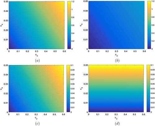
In Fig. 1a and (b), for a similar number of model evaluations to the AGR filter, the sampling error in the EnKF estimates are quite large. Note that the color bars in (a) and (b) are the same and are of a different order than the color bars used in (c) and (d). In panels (c) and (d), the amount error in the EnKF estimate with k = 100 and the AGR filter is comparable. The AGR filter quadrature error is invariant with respect to changes in c₂, whereas the EnKF estimation error depends on both c₂ and c₄ as expected given (3.20)(3.20) $${\mu }_1=〈x_1〉=c_2{\sigma }_0^2+\cdots$$(3.20) . If c₄, which the fourth derivative depends on, is sufficiently small we expect better performance from the AGR filter estimated mean (3.6) regardless of the size of c₂.

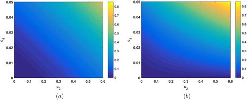
In the prior covariance estimates in Fig. 2, we see in (a) that the error in the EnKF covariance estimate with k = 100 grows with increases in c₂ and c₄. By comparison, the error in the AGR filter covariance in (b) is small when c₄ is small and grows as the fourth-order derivative grows as expected since the error depends on $c_4^2.$ The AGR filter covariance estimation is equal to or better than the EnKF estimate for small c₄. For larger c₄, the EnKF covariance estimate performs better. Note for this example we do not have a c₃ term which the error in the AGR filter and EnKF depends on as well.

Fig. 2. The L² error in (a) EnKF prior covariance estimate for k = 100 and (b) the error in the AGR filter prior covariance estimate for increasing values of c₂ (horizontal axis) and c₄ (vertical axis).

This example demonstrates the types of scenarios where one might choose one type of filter over another. For small ensemble sizes, the AGR filter may be the preferable choice as well as for the case where the model is moderately nonlinear, i.e. small magnitude higher order terms. For a large ensemble with large model fourth derivatives, the EnKF may provide a better estimate of the predicted mean.

3.5. Gaussian pdf integration: multi-dimensional case

We will now extend the results in Section 3.1 to higher dimensions. To evaluate integrals of the form (3.1), we begin by first applying the coordinate transform $x_{t-1}=S^T\eta +x_{t-1}^a,$ where S is the square root of the covariance $P_{t-1}^a$ such that $P_{t-1}^a=S^{T}S.$ Using this change of coordinates, we can convert (3.1) to the standard form with N(0, I), where I is the identity matrix. Then (3.22) $$\mathcal{I}={\int }_{{\mathbb{R}}^n}\tilde{F}(\eta )\frac{1}{{(2\pi )}^{n/2}}{e}^{-\frac{1}{2}|\eta {|}^2}\mathrm{d}\eta$$(3.22) where (3.23) $$\tilde{F}(\eta )=F(S^T\eta +x_{t-1}^a).$$(3.23)

Using (3.22)(3.22) $$\mathcal{I}={\int }_{{\mathbb{R}}^n}\tilde{F}(\eta )\frac{1}{{(2\pi )}^{n/2}}{e}^{-\frac{1}{2}|\eta {|}^2}\mathrm{d}\eta$$(3.22) we can develop formulas to evaluate (2.18) and (2.19)(2.19) $$P_t^b={\int }_{{\mathbb{R}}^n}(f(x_{t-1})-x_t^b){(f(x_{t-1})-x_t^b)}^{T}N(x_{t-1}|Y_{T-1})\mathrm{d}{x}_{t-1}+Q.$$(2.19) explicitly based on polynomial quadrature. In Ito and Xiong (2000), $\tilde{F}(\eta )$ is approximated by the function $\gamma (\eta )$ such that $\tilde{F}(z_i)=\gamma (z_i)$ for points $\left\{z_i\right\}$ in ${\mathbb{R}}^n.$ The multivariate polynomial $\gamma (\eta )$ is given by (3.24) $$\gamma (\eta )=\tilde{F}(0)+\sum _{i=1}^n{a}_i{s}_i+\frac{1}{2}\sum _{i=1}^n{b}_i{s}_i^2$$(3.24) where $a_i\in {\mathbb{R}}^n$ is the ith column of a, the first-order variation or Jacobian, s_i is the ith column of S, and b_i is the ith column approximation of the second-order variation, or Hessian. The coefficients a and b may be determined using centered differencing, similar to the scalar case, via (3.25) $$a_i=\frac{f(d{e}_i)-f(-d{e}_i)}{2d},1\le i\le n$$(3.25) where $\left\{e_i\right\}\in {\mathbb{R}}^n$ are unit vectors and d > 0. We approximate b_i via (3.26) $$b_i=\frac{f(d{e}_i)-2f(0)+f(-d{e}_i)}{d^2},1\le i\le n.$$(3.26)

Evaluating a and b requires $2n+1$ model evaluations. Note that we do not use cross derivative terms in the Hessian which would require an additional $\frac{1}{2}n(n-1)$ model evaluations to compute.

Using the polynomial in (3.24)(3.24) $$\gamma (\eta )=\tilde{F}(0)+\sum _{i=1}^n{a}_i{s}_i+\frac{1}{2}\sum _{i=1}^n{b}_i{s}_i^2$$(3.24) , we can write the integral (3.22)(3.22) $$\mathcal{I}={\int }_{{\mathbb{R}}^n}\tilde{F}(\eta )\frac{1}{{(2\pi )}^{n/2}}{e}^{-\frac{1}{2}|\eta {|}^2}\mathrm{d}\eta$$(3.22) as (3.27) $$\mathcal{I}={\int }_{{\mathbb{R}}^n}\gamma (\eta )\frac{1}{{(2\pi )}^{n/2}}{e}^{-1/2|\eta {|}^2}\mathrm{d}\eta$$(3.27) and create explicit formulas for the mean and covariance: (3.28) $$x_t^b={\int }_{{\mathbb{R}}^n}\gamma (\eta )\frac{1}{{(2\pi )}^{n/2}}{e}^{-1/2|\eta {|}^2}\mathrm{d}\eta$$(3.28) (3.29) $$=\frac{1}{{(2\pi )}^{n/2}}{\int }_{{\mathbb{R}}^n}\left(\tilde{F}(0)+\sum _{i=1}^n{a}_i{\eta }_i+\frac{1}{2}\sum _{i=1}^n{b}_i{\eta }_i^2\right)e^{-1/2|\eta {|}^2}\mathrm{d}\eta$$(3.29) (3.30) $$=f(x_{t-1}^a)+\frac{1}{2}\sum _{i=1}^n{b}_i$$(3.30) and (3.31) $$P_t^b=Q+{\int }_{{\mathbb{R}}^n}(\gamma (\eta )-x_t^b){(\gamma (\eta )-x_t^b)}^{\mathrm{T}}\frac{1}{{(2\pi )}^{n/2}}{e}^{-1/2|\eta {|}^2}\mathrm{d}\eta$$(3.31) (3.32) $$=Q+\frac{1}{{(2\pi )}^{n/2}}{\int }_{{\mathbb{R}}^n}\left(\sum _{i=1}^n{a}_i{\eta }_i+\frac{1}{2}\sum _{i=1}^n{b}_i{\eta }_i^2-\frac{1}{2}\sum _{i=1}^n{b}_i\right)$$(3.32) (3.33) $$·{\left(\sum _{i=1}^n{a}_i{\eta }_i+\frac{1}{2}\sum _{i=1}^n{b}_i{\eta }_i^2-\frac{1}{2}\sum _{i=1}^n{b}_i\right)}^{\mathrm{T}}{e}^{-1/2|\eta {|}^2}\mathrm{d}\eta$$(3.33) (3.34) $$=Q+\sum _{i=1}^n{a}_i{a}_i^T+\frac{1}{2}\sum _{i=1}^n{b}_i{b}_i^T.$$(3.34)

To summarize, a change of coordinates is used to transform the Gaussian integrals into standard form. We then approximate $\tilde{F}(s)$ by a quadratic polynomial. Using this approximation, we create self-contained formulas for the predicted mean and covariance.

Similar to the scalar case, odd polynomial terms drop out in the polynomial quadrature. This results in the quadrature error in estimating the mean (3.30)(3.30) $$=f(x_{t-1}^a)+\frac{1}{2}\sum _{i=1}^n{b}_i$$(3.30) on the order of the fourth derivative of the nonlinear model (see (B.8)(B.8) $$=\frac{1}{8}\sum _{i=1}^n{d}_{i,i,i,i}+\frac{1}{24}\sum _{i=j,k=\ell ,i\ne k}{d}_{i,i,k,k}+\frac{1}{24}\sum _{i=k,j=\ell ,i\ne j}{d}_{i,j,i,j}+\frac{1}{24}\sum _{i=\ell ,j=k,i\ne k}{d}_{i,j,j,i}+\cdots$$(B.8) in the appendix) even though our polynomial approximation (3.24)(3.24) $$\gamma (\eta )=\tilde{F}(0)+\sum _{i=1}^n{a}_i{s}_i+\frac{1}{2}\sum _{i=1}^n{b}_i{s}_i^2$$(3.24) is only second order. We do not see as much benefit in the computation of the covariance as the error given by (B.11)(B.11) $$=\frac{1}{4}\sum _{i\ne j}^n{b}_{ij}{b}_{ij}^{\mathrm{T}}+\frac{15}{36}\sum _{i=1}^n{c}_{\mathit{iii}}{c}_{\mathit{iii}}^{\mathrm{T}}+\frac{1}{36}\sum _{i\ne j\ne k}^n{c}_{\mathit{ijk}}{c}_{\mathit{ijk}}^{\mathrm{T}}+\cdots$$(B.11) is related to the cross terms in the Hessian approximation that were dropped in (3.24)(3.24) $$\gamma (\eta )=\tilde{F}(0)+\sum _{i=1}^n{a}_i{s}_i+\frac{1}{2}\sum _{i=1}^n{b}_i{s}_i^2$$(3.24) . Overall, the contribution to the filter error from the low-order polynomial quadrature is minimized for moderately nonlinear systems.

3.5.1 Multidimensional example

For this example, we will again look at the effects of nonlinearity versus sampling in the AGR filter and the EnKF. We consider a variable coefficient Korteweg-de Vries (KdV) model that governs the evolution of Rossby waves in a jet flow (Hodyss and Nathan, 2002). 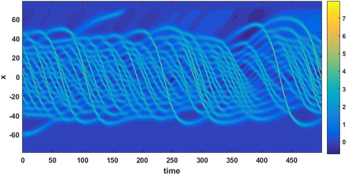This may be written as (3.35) $$A_t-A_{\mathit{xxxx}}+m_p(x)A_x+m_g(x)-A{A}_x=0$$(3.35) where $$\begin{array}{ccc}mp(x)& =& 1-\hspace{0.17em}\text{exp}\hspace{0.17em}(-a{x}^2)\\ m_g(x)& =& -2ax\hspace{0.17em}\text{exp}\hspace{0.17em}(-a{x}^2)\end{array}$$ and a = 0.0005. The derivatives are vanishing on the boundary, the initial condition is given by a solitary Rossby wave, and we use 512 model computational nodes. A contour plot of the true solution in time is shown in Fig. 3.

Fig. 3. Contour plot of the wave amplitude over the domain (vertical axis) of the KdV equation over time (horizontal axis).

We begin by creating a 35,000 member ensemble that will be used as the true solution in our experiments. This ensemble was created by drawing the members from climatology then using an EnKF to perform three system cycles using observations created from an ensemble member. This was done to improve the quality of the ensemble. The resulting covariance $P_0^b$ of this ensemble has eigenvalues plotted in Fig. 4.

Fig. 4. The 512 sorted eigenvalues of the initial background error covariance $P_0^b$ created from a 35000 member climatological ensemble. The horizontal axis is the eigenvalue number and the vertical axis is the magnitude of each eigenvalue.

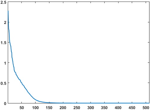
The eigenvalues of $P_0^b$ and their corresponding eigenvectors will be used to form $S=\sqrt{P}$ needed by the AGR filter. Additionally, members for smaller ensemble sizes will be drawn randomly from the 35,000-member ensemble. Since $P_0^b$ has near-zero eigenvalues, we will consider only the first 250 eigen-directions thus $$P_0^b\approx U_m{\Sigma }_m{U}_m^{\mathrm{T}}$$ where Σ_m is a truncated matrix with the first 250 eigenvalues of $P_0^b$ along the diagonal and U_m is composed of the corresponding eigenvectors. The square root of $P_0^b$ is then given by $S_m=U_m\sqrt{{\Sigma }_m}$ which is used in the coordinate transform (3.23)(3.23) $$\tilde{F}(\eta )=F(S^T\eta +x_{t-1}^a).$$(3.23) . In this example, 501 model evaluations are used to compute (3.30) and (3.34)(3.34) $$=Q+\sum _{i=1}^n{a}_i{a}_i^T+\frac{1}{2}\sum _{i=1}^n{b}_i{b}_i^T.$$(3.34) , thus the solution will be compared to an ensemble with 500 members for fairness. Similar to the one-dimensional example, the error in the prior mean estimates of the AGR filter and the EnKF is examined as nonlinearity is increased. The nonlinearity is further developed by increasing the amount of time (t₀) the model is integrated forward.

One way to observe the impact of the increased nonlinearity is to look at the influence of b in (3.24). For comparison we consider the filter without the second-order correction term which uses the first-order polynomial quadrature as AGR1, and with b which uses the second-order polynomial quadrature as AGR2.

Both filters are initialized using the mean of the 35,000 member ensemble, which we consider to be the true mean. The perturbations for the 500 member ensemble are drawn from the 35,000 member ensemble and then re-centered on the true mean. The S for the AGR filters is described above. All methods are integrated forward to t₀ and the prior means and covariances are computed. Fig. 5a compares the L₂ error in the EnKF prior mean solution with K = 500 and the AGR filter solutions with m = 250. The AGR2 filter significantly outperforms the AGR1 filter, demonstrating the importance of the second-order correction term. The AGR2 filter outperforms the EnKF until about $t_0=0.55$ or 5501 model time steps. The AGR2 filter performs well prior to this point having half the error of the EnKF at $t_0=0.25$ or 2501 model time steps. Fig. 5b compares the covariances of the EnKF and AGR filter using the Frobenius norm given by $$\left|\right|A|{|}_{\text{FRO}}=\sqrt{t\mathit{\text{race}}(A^{\mathrm{T}}A)}.$$

Fig. 5. (a) The L₂ error (vertical axis) in the estimate of the prior mean for the EnKF with k = 500, the AGR1 with m = 250, and AGR2 with m = 250 for time step length t₀ (horizontal axis). (b)The error in the Frobenius norm of the corresponding covariance estimates.

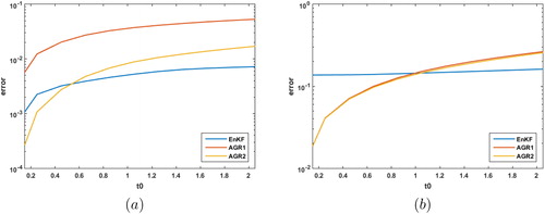
The AGR1 and AGR2 filters have about the same error in their covariances and outperform the EnKF until about $t_0=1.$ For model regimes which do not have overly large higher order terms, the AGR2 may provide better estimation.

For large n, evaluating (3.30) and (3.34)(3.34) $$=Q+\sum _{i=1}^n{a}_i{a}_i^T+\frac{1}{2}\sum _{i=1}^n{b}_i{b}_i^T.$$(3.34) is prohibitively expensive since it requires $2n_e+1$ model evaluations where n_e is the number of nonzero eigenvalues. To reduce the computational cost, we consider the case where only the leading m eigenvalues are kept. Ideally, m would be chosen so that the singular values capture the essential dynamics, however, in atmospheric applications this is may not be possible due to computational constraints. The truncation error in the estimation of the square root S_m of $P_{t-1}^a$ is given by (3.36) $$|S-S_m|\le \sum _{i>m}\sqrt{{\sigma }_i}.$$(3.36)

If $P_{t-1}^a$ has n–m eigenvalues approaching zero this estimation is very accurate. In other words, the extent of the correlations in $P_{t-1}^a$ determines the accuracy of this truncation. The error in evaluating (3.30) and (3.34)(3.34) $$=Q+\sum _{i=1}^n{a}_i{a}_i^T+\frac{1}{2}\sum _{i=1}^n{b}_i{b}_i^T.$$(3.34) now comes from both quadrature and this truncation.

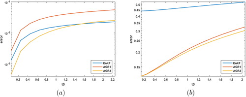
We repeat the previous experiment with K = 40 introducing undersampling for the EnKF estimate and m = 20 for the AGR estimates. Again we see the importance of the second-order correction term when comparing AGR1 and AGR2 in Fig. 6a. In (a) the AGR2 filter again has half the error of the EnKF at $t_0=0.25.$ However, due to the presence of sampling error in both of the prior mean estimates, the AGR2 continues to outperform the EnKF until about $t_0=1.55$ or 15,501 model time steps after which time the EnKF has a slight edge in performance. In (b) both the AGR1 and AGR2 estimates outperform the EnKF covariance estimates for various values of t₀.

Fig. 6. (a) The L₂ error (vertical axis) in the estimate of the prior mean for the EnKF with k = 40, the AGR1 with m = 20, and AGR2 with m = 20 for time step length t₀ (horizontal axis). (b) The corresponding error in the Forbenius norm for the prior covariance estimates.

In both the cases with undersampling and without undersampling the AGR2 consistently outperformed AGR1 due to the inclusion of the second-order correction term b. Additionally, in both cases, there was a moderately nonlinear regime in which the AGR2 filter outperformed the EnKF. Similar to the scalar case, the AGR2 filter was found to be more sensitive to increased nonlinearity than the EnKF; however, the EnKF proved to be more sensitive to undersampling. This broadened the regime in which the AGR2 filter outperformed the EnKF.

3.5.2 A note on $P_0^b$

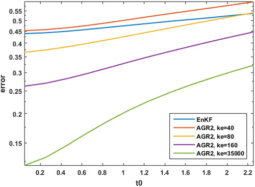
For this example, S_m was computed from $P_0^b$ for the AGR filters. This $P_0^b$ was created using a 35,000 member climatological ensemble. Using fewer ensemble members to create $P_0^b$ introduces another source of error at the starting time. For example, if $P_0^b$ is constructed with $k_e=40,80,160,35000$ ensemble members, then the accuracy of the AGR2 filter for m = 20 decreases accordingly for computing the prior covariance estimates as in Fig. 7. For convenience, we have included the error estimate for the EnKF in this plot. Note that the ensemble of the 40 member EnKF is drawn from the 35,000 member climatological ensemble. There are numerous strategies to develop a more accurate and higher rank $P_0^b$ (Clayton et al., 2013; Derber and Bouttier, 1999) which are beyond the scope of this paper.

Fig. 7. The error in the Frobenius norm (vertical axis) of the prior covariance estimates in the AGR2 filter for m = 20 with $P_0^b$ computed using $k_e=40,80,160,35000$ ensemble members for time step length t₀ (horizontal axis).

4 AGR filters

In order to utilize the mean (3.30)(3.30) $$=f(x_{t-1}^a)+\frac{1}{2}\sum _{i=1}^n{b}_i$$(3.30) and covariance (3.34)(3.34) $$=Q+\sum _{i=1}^n{a}_i{a}_i^T+\frac{1}{2}\sum _{i=1}^n{b}_i{b}_i^T.$$(3.34) updates, we develop an algorithm in the same vein as the ensemble square root filters (Whitaker and Hamill, 2002), i.e. we will update S_m keeping P^b in factored form. To begin with we note that after some algebraic manipulation and dropping Q, we may rewrite (3.34)(3.34) $$=Q+\sum _{i=1}^n{a}_i{a}_i^T+\frac{1}{2}\sum _{i=1}^n{b}_i{b}_i^T.$$(3.34) as (4.1) $$P_t^b=a\left(I+{\left(a^{\mathrm{T}}{\left(\frac{1}{2}b{b}^{\mathrm{T}}\right)}^{-1}a\right)}^{-1}\right)a^{\mathrm{T}}.$$(4.1) where $a=[a_1,\dots ,a_m]$ and $b=[b_1,\dots ,b_m]$ are computed using the centered differencing scheme (4.2) $$a_i=\frac{f(S^T(d{e}_i)+x_{t-1}^a)-f(S^{\mathrm{T}}(-d{e}_i)+x_{t-1}^a)}{2d},1\le i\le m$$(4.2) and we approximate b_i via (4.3) $$b_i=\frac{f(S^T(d{e}_i)+x_{t-1}^a)-2f(x_{t-1}^a)+f(S^{\mathrm{T}}(-d{e}_i)+x_{t-1}^a)}{d^2},1\le i\le m.$$(4.3)

The above equations are the same as (3.25) and (3.26)(3.26) $$b_i=\frac{f(d{e}_i)-2f(0)+f(-d{e}_i)}{d^2},1\le i\le n.$$(3.26) but with the truncated S = S_m. Letting $\xi =\sqrt{2}{b}^{†}a,$ where $b^{†}$ is the Moore-Penrose pseudo inverse, and using (4.1)(4.1) $$P_t^b=a\left(I+{\left(a^{\mathrm{T}}{\left(\frac{1}{2}b{b}^{\mathrm{T}}\right)}^{-1}a\right)}^{-1}\right)a^{\mathrm{T}}.$$(4.1) , then $P=\tilde{a}{\tilde{a}}^T$ where (4.4) $$\tilde{a}=a\sqrt{I+{({\xi }^T\xi )}^{-1}}.$$(4.4)

Note that $\xi \in {\mathbb{R}}^m$ so the expression in (4.4)(4.4) $$\tilde{a}=a\sqrt{I+{({\xi }^T\xi )}^{-1}}.$$(4.4) may not be overly expensive to compute. To form the filter, we use the Potter method (Potter, 1963) for the Kalman square root update in reduced order form. This will improve the numerical robustness by ensuring $P=S^{\mathrm{T}}S$ is symmetric and reducing the amount of storage required by the AGR filter by only storing the square root S. To form the filter, let (4.5) $$\beta =H\tilde{a}\in R^{p\times m}$$(4.5) then (4.6) $$Z=R+H{P}^b{H}^{\mathrm{T}}=R+\beta {\beta }^{\mathrm{T}},K_t=\tilde{a}{\beta }^{\mathrm{T}}{Z}^{-1}.$$(4.6)

Thus, $$P_t^a=\tilde{a}(I-{\beta }^T{Z}^{-1}\beta ){\tilde{a}}^T.$$

Letting $\eta =I-{\beta }^T{Z}^{-1}\beta =VD{V}^T$ then we update S by $$S_t=(\sqrt{D}+ϵI)V^{\mathrm{T}}\tilde{a}$$ where $ϵ>0$ is a tunable parameter. We have chosen to form a regularized S which will help with the conditioning of the matrix and decrease dispersion. Other inflation methods such as multiplicative covariance inflation may also be used. To summarize, the algorithm for the AGR2 filter is as follows:

1. Given $S_{t-1}=[s_1,\dots ,s_m]$ compute $x_t^b$ and a_i, b_i for $1\le i\le m.$

2. Compute $\tilde{a}$ as in (4.4).

3. Let $\beta =H\tilde{a}$ then $$x_t^a=x_t^b+K_t(y_t-H{x}_t^b)$$

where $$K_t=\tilde{a}{\beta }^T{Z}^{-1}$$ and $$Z=R+\beta {\beta }^T.$$

1. Decompose η such that $\eta =VD{V}^T$ where D is diagonal and V is unitary. Then $S_t=(\sqrt{D}+ϵI)V^T\tilde{a}.$

The algorithm itself is readily implemented and requires minimal tuning of the parameter d from Equations (4.2)(4.2) $$a_i=\frac{f(S^T(d{e}_i)+x_{t-1}^a)-f(S^{\mathrm{T}}(-d{e}_i)+x_{t-1}^a)}{2d},1\le i\le m$$(4.2) and (4.3)(4.3) $$b_i=\frac{f(S^T(d{e}_i)+x_{t-1}^a)-2f(x_{t-1}^a)+f(S^{\mathrm{T}}(-d{e}_i)+x_{t-1}^a)}{d^2},1\le i\le m.$$(4.3) . For quasi-linear systems, the second-order correction term b may be dropped giving the AGR1 filter. In this case, we may further reduce computational cost by using finite differencing instead of centered differencing. Then to evaluate (3.30) and (3.34)(3.34) $$=Q+\sum _{i=1}^n{a}_i{a}_i^T+\frac{1}{2}\sum _{i=1}^n{b}_i{b}_i^T.$$(3.34) , we use the finite differencing scheme to approximate the $a_i,i=1,\dots ,m,$ i.e., (4.7) $$a_i=\frac{f(S^T(d{e}_i)+x_{t-1}^a)-f(x_{t-1}^a)}{d},1\le i\le m$$(4.7) after the coordinate change where d > 0 is the step size. The benefit of computing a_i in this manner is that this only requires m + 1 model evaluations. Note that the expression (4.7)(4.7) $$a_i=\frac{f(S^T(d{e}_i)+x_{t-1}^a)-f(x_{t-1}^a)}{d},1\le i\le m$$(4.7) amounts to a directional derivative determined by the truncated S. In using S the derivative is computed in the direction of the largest change in the dynamics. Meanwhile, the parameter d restricts the search direction to a constrained set. This is a generalization of the standard derivative, in fact it is a numerical approximation of the Jacobian under a coordinate transformation. In this way, the AGR1 may be viewed as a form of an extended Kalman filter.

5. Data assimilation

In this section, we present data assimilation comparisons between the AGR2 filter, described in the previous section, and the ensemble square root filter (Tippett et al., 2003) as the example EnKF method. We use this particular filter as the correction step as it is most similar to the AGR filter while having an ensemble estimate for the mean and covariance.

5.1. 1 D Example

We return to the KdV model given by (3.35)(3.35) $$A_t-A_{\mathit{xxxx}}+m_p(x)A_x+m_g(x)-A{A}_x=0$$(3.35) . As before we will use k = 40 ensemble members drawn from the 35,000 member ensemble for the EnKF and the AGR2 filter with m = 20. This time the initial $x_0^a$ for the AGR2 filter will be the mean of the k = 40 EnKF ensemble. Both the EnKF and AGR2 filter will use the same 32 observations at assimilation time. We use localization and multiplicative inflation wherein the correlation length scale used in the localization and the inflation factor were tuned so that the ensemble variance correspond to the true error variance. We again consider different values of t₀, the time the model is integrated forward before assimilation, to see how increasing the nonlinearity affects these two filtering algorithms. To reduce the influence of the initial conditions, we will only consider assimilation cycles 200–450.

Figure 8 is a plot of the average error across a data assimilation window for various t₀. For smaller t₀ the model integration is less nonlinear and we can see that the AGR2 filter has about 30% less error than the EnKF. As t₀ gets larger, the model integration is more nonlinear and the error in the solution of the AGR2 grows more rapidly than the EnKF and by $t_0=2.05$ or 20001 model time steps the AGR2 error is about 24% less than the EnKF.

Fig. 8. The L² error (vertical axis) averaged over the assimilation window for increasing t₀ (horizontal axis), the time between cycles, for the EnKF and the AGR2 filter.

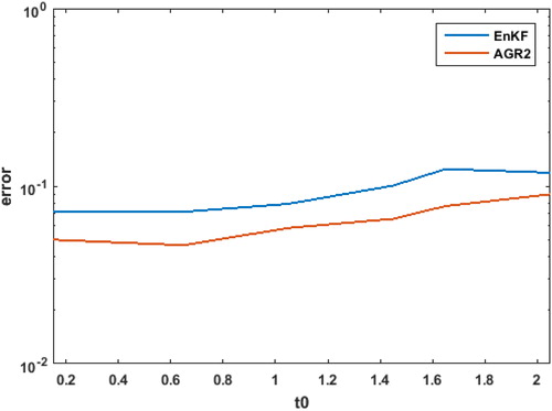
This cycling experiment result demonstrates that the improvement in the predicted mean and covariance estimates seen in Fig. 6 leads to an improvement in the data assimilation state estimation or analysis. Also it demonstrates that increasing the nonlinearity has more of an impact on the quality of the AGR2 solution versus the EnKF solution.

5.2. 2 D Example

We will now investigate the performance of the proposed AGR filter using a two-dimensional Boussinesq model that develops Kelvin-Helmhotz waves, specifically, we use the model developed in (Hodyss et al., 2013). The governing equations given by (5.1) $$\begin{array}{ccc}\frac{\partial \zeta }{\partial t}& =& -\left(u\frac{\partial \zeta }{\partial x}+w\frac{\partial \zeta }{\partial z}+\frac{g}{{\theta }_0}\frac{\partial \theta }{\partial x}\right)+F,\\ \frac{\partial \theta }{\partial t}& =& -\left(u\frac{\partial \theta }{\partial x}+w\frac{\partial \theta }{\partial z}+w\frac{\partial {\theta }_0}{\partial z}\right)+H,\end{array}$$(5.1) where $$u=\frac{\partial \psi }{\partial z},w=-\frac{\partial \psi }{\partial x},\text{and}\zeta ={\nabla }^2\psi ,$$

${\nabla }^2$ is the Laplacian operator, u and w are zonal and vertical winds, respectively, θ is the potential temperature, and ζ is the vorticity. The vorticity source F and the heat source H both have sub-grid scale parameterizations, more details may be found in Hodyss et al. (2013). 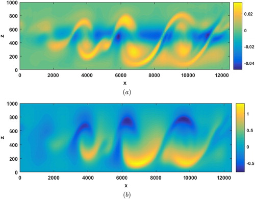The buoyancy frequency of the reference state ${\Theta }_0$ is given by the background potential temperature: $N_0^2=\frac{g}{{\theta }_0}\frac{d{\theta }_0}{dz}={10}^{-4}{s}^{-1}.$ And $$U_0=\frac{V}{2}\left[1+\tanh \left(\mu \frac{z-z_0}{L}\right)\right]$$ is the reference state for the zonal wind with $V=10m{s}^{-1},$ μ = 8, L = 1 km, and $z_0=0.5$ km. The z boundary conditions are a mirrored forcing the vertical velocity to vanish. Additionally, there are sponge boundaries along the left and right sides of the channel. At time t = 0, the flow is perturbed leading to waves that amplify as they travel then break. For this experiment, the model was run with 128 computational nodes in the x direction and 33 nodes (unmirrored) in the z direction. All told the state vector has 8448 elements. The true solution at the end of the assimilation window may be seen in Fig. 9 for (a) the vorticity and (b) the temperature. As the waves move across the atmospheric slice, they grow and eventually shear.

Fig. 9. The true solution of (5.1) at time t = 15000, or 200 cycles of 75 seconds, for (a) vorticity and (b) temperature. The vertical axis is the height and the horizontal axis is the distance.

During the assimilation window, the model is advanced, then the filtering is performed with 112 temperature and 112 wind observations. The observations are created by perturbing the truth via (5.2) $$y_t=y_t^{\text{true}}+R^{1/2}{\xi }_t$$(5.2) where R is the instrument error covariance and ξ is white noise. For this experiment, $R=1e-2$ for both the temperature and wind. A 24,000 member ensemble was created by cycling random perturbations through the model. The smaller k = 20 and k = 40 ensembles were drawn from this 24,000 member ensemble and which was also used to create $P_0^b$ for the AGR filter. We initialize the $x_0^a$ used in the AGR filter with the mean of the k = 20 ensemble for the EnKF. Both the EnKF with k = 20, 40 and the AGR2 filter will use the same observations for a particular t₀. Again both types of filters are using localization and inflation tuned to so that the ensemble variance matches the true error variance. We will compute the error averaged over assimilation cycles 100–400 to reduce the influence of the initial conditions.

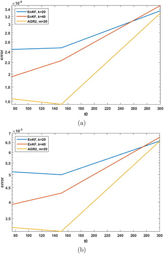
The error in the mean estimation plots in Fig. 10a and b demonstrate similar results to the one-dimensional KdV example. For the more linear case $t0=75,$ the AGR2 filter significantly outperforms the EnKF. As t₀ is increased, the nonlinearity increases and the AGR2 filter loses its performance advantage over the EnKF until around $t0=300.$ As before, the increased nonlinearity has a greater impact on the performance of the AGR2 filter as opposed to the EnKF.

Fig. 10. The averaged L² error (vertical axis) across the data assimilation window in the mean estimates for particular t₀ (horizontal axis) for (a) vorticity and (b) temperature.

We have presented two example problems comparing the AGR filter and the EnKF. The first example was a one-dimensional KdV model in which the AGR filter outperformed the EnKF but was more influenced by nonlinearity. In the second example, a two-dimensional Boussinesq model was considered. In this case, starting with $t0=75,$ the AGR filter out performed the EnKF. When $t0=300,$ the error in the mean estimation has more than doubled and the performance between the AGR filter and the EnKF are comparable. Again we see that the AGR filter is more affected by the nonlinearity in the model than the EnKF.

6. Final remarks

We have presented a quadrature Kalman filter, the AGR filter, for moderately nonlinear systems. The filter uses numerical quadrature to evaluate the Bayesian formulas for optimal filtering under Gaussian assumptions. The AGR filter has the Gaussian noise assumptions and Gaussian joint distribution assumption from Kalman filtering with the added assumption that the prior distribution is Gaussian. This leads to Gaussian integrals which are evaluated using the second-order polynomial quadrature. Due to the properties of Gaussian distributions, using this polynomial achieves the same precision as a third-order polynomial quadrature. This effective higher order quadrature is key to the success of this filter.

In numerical tests, the AGR filter was found to outperform a comparable square-root EnKF in regions of low-to-moderate nonlinearity for a KdV model and a Boussinesq model. We expect these results to extend to more realistic atmospheric models, given that fourth and higher order terms of the model are sufficiently small. For highly nonlinear dynamical systems, the AGR filter is affected more than the square-root EnKF but may still provide performance benefit if the system is severely under-sampled as demonstrated in the scalar example in Section 3.4. It is also possible to use higher order quadrature to reduce the effect of nonlinearity but this would, of course, increase the computational costs of the filter.

While the Gaussian assumption made in this filter may seem restrictive, this assumption is commonly made, or effectively made, in data assimilation. For example, recent results indicate that it may require an ensemble with on the order of one thousand members to capture non-Gaussianity pdfs present in an EnKF for a simplified general circulation model (Miyoshi et al., 2014). This is already significantly more than the O(100) ensemble members typically used in EnKFs for full complexity atmospheric models. Effectively, a Gaussian assumption is being made due to the sample size. The computational efficiency of the AGR filter means that there is greater opportunity to pursue non-Gaussian pdfs via Gaussian mixture models (GMMs). In GMMs a non-Gaussian distribution is approximated by a series of Gaussian distributions which, in this case, would lead to an optimally weighted ensemble of AGR filters.

A. Formulas

A.1. Expectation formulas

Consider the expectation (A.1) $$E[x_t,Y_{T-1}]={\int }_{{\mathbb{R}}^n}{x}_{t}p(x_t|Y_{T-1})\mathrm{d}{x}_t$$(A.1) (A.2) $$={\int }_{{\mathbb{R}}^n}\left[{\int }_{{\mathbb{R}}^n}{x}_{t}p(x_t|x_{t-1})d{x}_t\right]p(x_{t-1}|Y_{T-1})\mathrm{d}{x}_{t-1}$$(A.2) (A.3) $$={\int }_{{\mathbb{R}}^n}f(x_{t-1})p(x_{t-1}|Y_{T-1})\mathrm{d}{x}_{t-1}$$(A.3)

where $E[·]$ is the expectation. Note that (A.2)(A.2) $$={\int }_{{\mathbb{R}}^n}\left[{\int }_{{\mathbb{R}}^n}{x}_{t}p(x_t|x_{t-1})d{x}_t\right]p(x_{t-1}|Y_{T-1})\mathrm{d}{x}_{t-1}$$(A.2) follows from (2.1)(2.1) $$p(x_t|Y_{T-1})=\int p(x_t|x_{t-1})p(x_{t-1}|Y_{T-1})\mathrm{d}{x}_{t-1}.$$(2.1) and Fubini’s theorem and (2.7)(2.7) $$={\int }_{{\mathbb{R}}^n}f(x_{t-1})p(x_{t-1}|Y_{T-1})\mathrm{d}{x}_{t-1}$$(2.7) follows from (2.3)(2.3) $$x_t=f(x_{t-1})+w_t$$(2.3) and w_t being Gaussian. Similarly, the predicted covariance is given by (A.4) $$E\left[x_t{x}_t^T\right]={\int }_{{\mathbb{R}}^n}{x}_t{x}_t^{T}p(x_t|Y_{T-1})\mathrm{d}{x}_t$$(A.4) (A.5) $$={\int }_{{\mathbb{R}}^n}\left[{\int }_{{\mathbb{R}}^n}{x}_t{x}_t^{T}p(x_t|x_{t-1})d{x}_t\right]p(x_{t-1}|Y_{T-1})\mathrm{d}{x}_{t-1}$$(A.5) (A.6) $$={\int }_{{\mathbb{R}}^n}f(x_{t-1})f{(x_{t-1})}^{T}p(x_{t-1}|Y_{T-1})\mathrm{d}{x}_{t-1}+Q.$$(A.6)

A.2. Covariance

The cross covariance in (2.13)(2.13) $$=N\left(\left(\begin{array}{c}{x_t}^b\\ {{\hat{y}}_t}^b\end{array}\right),\left(\begin{array}{cc}{P_t}^b& {P_t}^b{H}^T\\ H{P_t}^b& H{P_t}^b{H}^T+R\end{array}\right)\right)$$(2.13) is computed via (A.7) $$P_t^{xy}=E[(x_t-x_t^b){({\widehat{y}}_t-{\widehat{y}}_t^b)}^{\mathrm{T}}]$$(A.7) (A.8) $$=\int (x_t-x_t^b){({\widehat{y}}_t-{\widehat{y}}_t^b)}^{T}p(x_t,{\widehat{y}}_t|Y_{t-1})\mathrm{d}{x}_t\mathrm{d}{\widehat{y}}_t$$(A.8) (A.9) $$={\int }_{{\mathbb{R}}^n}(x_t-x_t^b)\left[{\int }_{{\mathbb{R}}^d}{({\widehat{y}}_t-{\widehat{y}}_t^b)}^{T}p({\widehat{y}}_t|x_t)\mathrm{d}{\widehat{y}}_t\right]p(x_t|Y_{T-1})\mathrm{d}{x}_t$$(A.9) (A.10) $$={\int }_{{\mathbb{R}}^n}(x_t-x_t^b){(H{x}_t-H{x}_t^b)}^{\mathrm{T}}p(x_t|Y_{t-1})\mathrm{d}{x}_t$$(A.10) (A.11) $$={\int }_{{\mathbb{R}}^n}(x_t-x_t^b){(x_t-x_t^b)}^{\mathrm{T}}{H}^{\mathrm{T}}p(x_t|Y_{t-1})\mathrm{d}{x}_t$$(A.11) (A.12) $$=P_t^b{H}^T.$$(A.12)

B. Qquadrature error

B.1. Scalar quadrature error

The quadrature error in evaluating the integrals (2.18) and (2.19)(2.19) $$P_t^b={\int }_{{\mathbb{R}}^n}(f(x_{t-1})-x_t^b){(f(x_{t-1})-x_t^b)}^{T}N(x_{t-1}|Y_{T-1})\mathrm{d}{x}_{t-1}+Q.$$(2.19) comes from the low-order polynomial approximation (3.2)(3.2) $$\gamma (s)=\tilde{F}(0)+a_{1}s+\frac{1}{2}{a}_2{s}^2$$(3.2) . Consider the estimation error of (3.6)(3.6) $$=f(x_{t-1}^a)+\frac{1}{2}{a}_2.$$(3.6) given by (B.1) $$e_{\text{mean}}={\int }_{\mathbb{R}}(f(\sqrt{P}\eta +x_{t-1}^a)-\gamma (\eta ))N(\eta |0,1)\mathrm{d}\eta$$(B.1) (B.2) $$={\int }_{\mathbb{R}}(\frac{1}{6}{a}_3{\eta }^3+\frac{1}{24}{a}_4{\eta }^4+\cdots )\frac{1}{\sqrt{2\pi }}{e}^{-\frac{1}{2}{\eta }^2}\mathrm{d}\eta$$(B.2) (B.3) $$=\frac{3}{24}{a}_4+\cdots$$(B.3) where $a_3,a_4$ are the third and fourth derivatives, respectively, of f. Similarly, the quadrature error for (3.9)(3.9) $$=a_1^2+\frac{1}{2}{a}_2^2+Q.$$(3.9) is given by (B.4) $$e_{\text{covariance}}={\int }_{\mathbb{R}}(f(\sqrt{P}\eta +x_{t-1}^a)-x_{t-1}^a{)}^{2}N(\eta |0,1)\mathrm{d}\eta$$(B.4) (B.5) $$={\int }_{\mathbb{R}}{\left(\frac{1}{6}{a}_3{\eta }^3+\frac{1}{24}{a}_4{\eta }^4+\cdots -\left(\frac{3}{24}{a}_4+\cdots \right)\right)}^2\frac{1}{\sqrt{2\pi }}{e}^{-\frac{1}{2}{\eta }^2}\mathrm{d}\eta$$(B.5) (B.6) $$=\frac{15}{36}{a}_3^2+\frac{105}{576}{a}_4^2+\cdots .$$(B.6)

B.2. N-d quadrature error

The estimation error of (3.30) and (3.34)(3.34) $$=Q+\sum _{i=1}^n{a}_i{a}_i^T+\frac{1}{2}\sum _{i=1}^n{b}_i{b}_i^T.$$(3.34) is given by (B.7) $$e_{\text{mean}}=\frac{1}{{(2\pi )}^{n/2}}{\int }_{{\mathbb{R}}^n}\left(\frac{1}{2}\sum _{i\ne j}^n{b}_{i,j}{\eta }_i{\eta }_j+\frac{1}{6}\sum _{i,j,k=1}^n{c}_{i,j,k}{\eta }_i{\eta }_j{\eta }_k+\frac{1}{24}\sum _{i,j,k,\ell =1}^n{d}_{i,j,k,\ell }{\eta }_i{\eta }_j{\eta }_k{\eta }_{\ell }\cdots \right)e^{-1/2|\eta {|}^2}\mathrm{d}\eta$$(B.7) (B.8) $$=\frac{1}{8}\sum _{i=1}^n{d}_{i,i,i,i}+\frac{1}{24}\sum _{i=j,k=\ell ,i\ne k}{d}_{i,i,k,k}+\frac{1}{24}\sum _{i=k,j=\ell ,i\ne j}{d}_{i,j,i,j}+\frac{1}{24}\sum _{i=\ell ,j=k,i\ne k}{d}_{i,j,j,i}+\cdots$$(B.8) and (B.9) $$e_{\text{covariance}}=\frac{1}{{(2\pi )}^{n/2}}{\int }_{{\mathbb{R}}^n}\left(\frac{1}{2}\sum _{i\ne j}^n{b}_{i,j}{\eta }_i+\frac{1}{6}\sum _{i,j,k=1}^n{c}_{i,j,k}{\eta }_i{\eta }_j{\eta }_k+\cdots -\left(\frac{1}{8}\sum _{i=1}^n{d}_{i,i,i,i}+\cdots \right)\right)$$(B.9) (B.10) $$·{\left(\frac{1}{2}\sum _{i\ne j}^n{b}_{i,j}{\eta }_i+\frac{1}{6}\sum _{i,j,k=1}^n{c}_{i,j,k}{\eta }_i{\eta }_j{\eta }_k+\cdots -\left(\frac{1}{8}\sum _{i=1}^n{d}_{i,i,i,i}+\cdots \right)\right)}^{\mathrm{T}}{e}^{-1/2|\eta {|}^2}d\eta$$(B.10) (B.11) $$=\frac{1}{4}\sum _{i\ne j}^n{b}_{ij}{b}_{ij}^{\mathrm{T}}+\frac{15}{36}\sum _{i=1}^n{c}_{\mathit{iii}}{c}_{\mathit{iii}}^{\mathrm{T}}+\frac{1}{36}\sum _{i\ne j\ne k}^n{c}_{\mathit{ijk}}{c}_{\mathit{ijk}}^{\mathrm{T}}+\cdots$$(B.11) where $$c_{\mathit{ijk}}=\sum _{i,j,k=1}^n\frac{{\partial }^{3}f}{\partial x_i\partial x_j\partial x_k}\text{and}{d}_{\mathit{ijk}\ell }=\sum _{i,j,k,\ell =1}^n\frac{{\partial }^{4}f}{\partial x_i\partial x_j\partial x_k\partial x_{\ell }}.$$

Note that the error on the mean does not depend on the cross terms in the Jacobian.

Acknowledgments

The authors would like to express their gratitude to Dr Nancy Baker from the U.S. Naval Research Laboratory for her insights and discussions that have greatly improved this manuscript. This research is supported by the Office of Naval Research (ONR) through the NRL Base Program PE 0601153N.

References

- Anderson, J. L. 2001. An ensemble adjustment filter for data assimilation. Mon. Wea. Rev. 129, 2884–2903. doi:10.1175/1520-0493(2001)129<2884:AEAKFF>2.0.CO;2
- Arasaratnam, I. and Haykin, S. 2009. Cubature Kalman filters. IEEE Trans. Automat. Contr. 54, 1254–1269. doi:10.1109/TAC.2009.2019800
- Bishop, C. H., Etherton, B. and Majumdar, S. J. 2001. Adaptive sampling with the ensemble transform Kalman filter, Part I: theoretical aspects. Mon. Wea. Rev. 129, 420–1167. doi:10.1175/1520-0493(2001)129<0420:ASWTET>2.0.CO;2
- Buehner, M., Houtekamer, P. L., Charette, C., Mitchell, H. L. and He, B. 2010. Intercomparison of variational data assimilation and the ensemble Kalman filter for global deterministic NWP. Part II: one-month experiments with real observations. Mon. Wea. Rev. 138, 1567–1586. doi:10.1175/2009MWR3158.1
- Chen, Z. 2003. Bayesian Filtering: From Kalman Filters to Particle Filters, and Beyond. Tech. Rep. Hamilton, Canada: McMaster University.
- Clayton,A. M., Lorenc, A. C. and Barker, D. M. 2013. Operational implementation of a hybrid ensemble/4D-Var global data assimilation system at the Met Office. Qjr. Meteorol. Soc. 139, 1445–1461. doi:10.1002/qj.2054
- Courtier, P., Andersson, E., Heckley, W., Pailleux, J., Vasiljevic̀, D. and co-authors. 1998. The ECMWF implementation of three-dimensional variational assimilation (3D-Var). I: formulation. Q. Q. J. Royal Met. Soc. 124, 1783–1807.
- Daley, R. 1991.Atmospheric Data Analysis. Cambridge University Press, New York.
- Derber, J. and Bouttier, F. 1999. A reformulation of the background error covariance in the ECMWF global data assimilation system. Tellus A 51, 195–221. doi:10.3402/tellusa.v51i2.12316
- Evensen, G. 2003. The ensemble Kalman filter: theoretical formulation and practical implementation. Ocean Dynamics 53, 343–367. doi:10.1007/s10236-003-0036-9
- Haykin, S., Zia, A., Xue, Y. and Arasaratnam, I. 2011. Control theoretic approach to tracking radar: first step towards cognition. Digit. Signal Process. 21, 576–585. doi:10.1016/j.dsp.2011.01.004
- Ho, Y. C. and Lee, R. C. K. 1964. A Bayesian approach to problems in stochastic estimation and control. IEEE Trans. Automat. Control 9, 333–339. doi:10.1109/TAC.1964.1105763
- Hodyss, D., Campbell, W. F. and Whitaker, J. S. 2016. Observation-dependent posterior inflation for the ensemble Kalman Filter. Mon. Wea. Rev. 144, 2667–2684. doi:10.1175/MWR-D-15-0329.1
- Hodyss, D. and Nathan, T. 2002. Solitary Rossby waves in zonally varying jet flows. Physica D96, 239–262.
- Hodyss, D., Viner, K., Reinecke, A. and Hansen, J. 2013. The impact of noisy physics on the stability and accuracy of physics-dynamics coupling. Mon. Wea. Rev. 144, 4470–4486.
- Houtekamer, P. L., Deng, X., Mitchell, H. L., Baek, S. J. and Gagnon, N. 2014. Higher resolution in operational ensemble Kalman Filter. Mon. Wea. Rev. 142, 1143–1162. doi:10.1175/MWR-D-13-00138.1
- Ito, K. and Xiong, K. 2000. Gaussian filters for nonlinear filtering problems. IEEE Trans. Automat. Control 45, 910–927. doi:10.1109/9.855552
- Julier, S., Uhlmann, J. and Durrant-Whyte, H. F. 2000. A new method for the nonlinear transformation of means and covariances in filters and estimators. IEEE Trans. Automat. Contr. 45, 477–482. doi:10.1109/9.847726
- King, S., Kang, W. and Ito, K. 2016. Reduced order Gaussian smoothing for nonlinear data assimilation. IFAC-Papers OnLine 49, 199–204. doi:10.1016/j.ifacol.2016.10.163
- Kalman, R. E. 1960. A new approach to linear filtering and prediction problems. Trans. ASME, J. Basic Eng. 82, 35–45. doi:10.1115/1.3662552
- Kuhl, D. D., Rosmond, T. E., Bishop, C. H., McLay, J. and Baker, N. L. 2013. Comparison of hybrid ensemble/4DVar and 4DVar within the NAVDAS-AR data assimilation framework. Mon. Wea. Rev. 141, 2740–2758. doi:10.1175/MWR-D-12-00182.1
- Liu, J., Cai, B. and Wang, J. 2017. Cooperative localization of connected vehicles: integrating GNSS with DSRC using a robust cubature Kalman filter. IEEE Trans. Intell. Transport. Syst. 18, 2111–2125. doi:10.1109/TITS.2016.2633999
- Morzfeld, M. and Hodyss, D. 2019. Gaussian approximations in filters and smoothers for data assimilation. Tellus A 71, 1–27.
- Miyoshi, T., Kondo, K. and Imamura, T. 2014. The 10,240-member ensemble Kalman filtering with an intermediate AGCM. Geophys. Res. Lett. 41, 5264–5271. doi:10.1002/2014GL060863
- Poterjoy, J. 2016. A localized particle filter for high-dimensional nonilnear systems. Mon. Wea. Rev. 144, 59–76. doi:10.1175/MWR-D-15-0163.1
- Potter, J. E. 1963. New Statistical Formulas. Space Guidance Analysis Memo 40, Instrumentation Laboratory, MIT, Cambridge, MA.
- Särkkä, S. 2013. Bayesian Filtering and Smoothing. Cambridge University Press, Cambridge.
- Sharma, A., Srivastava, S. C. and Chakrabarti, S. 2017. A cubature Kalman filter based power system dynamic stat estimator. IEEE Trans. Instrum. Meas. 66, 2036–2045. doi:10.1109/TIM.2017.2677698
- Sondergaard, T. and Lermusiaux, P. F. J. 2013. Data assimilation with Gaussian mixture models using the dynamically orthogonal field equations. Part I: theory and scheme. Mon. Wea. Rev. 141, 1737–1760. doi:10.1175/MWR-D-11-00295.1
- Talagrand, O. and Courtier, P. 1987. Variational assimilation of meteorological observations with the adjoint vorticity equation I: theory.Qjr. Meteorol. Soc.116, 1311–1328.
- Tippett, M. K., Anderson, J. L., Bishop, C. H., Hamill, T. M. and Whitaker, J. S. 2003. Ensemble square root filters. Mon. Wea. Rev. 131, 1485–1490. doi:10.1175/1520-0493(2003)131<1485:ESRF>2.0.CO;2
- Whitaker, J. S. and Hamill, T. M. 2002. Ensemble data assimilation without perturbed observations. Mon. Wea. Rev. 130, 1913–1924. doi:10.1175/1520-0493(2002)130<1913:EDAWPO>2.0.CO;2
- Wu, Y., Hu, D., Wu, M. and Hu, X. 2006. A Numerical-integration perspective on Gaussian filters. IEEE Trans. Signal Process. 54, 2910–2921. doi:10.1109/TSP.2006.875389