Impact of climate change on the climatology of Vb cyclones

Abstract

Extratropical cyclones of type Vb develop over the western Mediterranean and move north-eastward, leading to heavy precipitation over central Europe and posing a major natural hazard. Thus, this study aims at assessing their sensitivity to climate change and deepens the understanding of the underlying processes of Vb-type cyclones. The analysis is based on global climate model output, which is dynamically downscaled for extreme Vb cyclones. Thereby two periods are compared: the reference period 1979 to 2013, and the future period 2070 to 2099 under the representative concentration pathway RCP8.5. Additionally, we include the analysis from a large ensemble (LENS), where 25 ensemble members are analysed for the reference period 1990–2005 and the future period 2071–2080. The results show a reduction of Vb cyclones from 3.2 events per year during the reference period to only 2.1 Vb cyclones per year at the end of the 21st century. This result is supported by the LENS, which shows a significant reduction from 2.9 to 2.6 Vb events per year. This reduction is induced by a northward shift of cyclone track over Europe in the future. To gain insight into the impact of Vb cyclones, 10 Vb cyclones with the most intense precipitation over the Alps are selected and dynamically downscaled for each period, separately. Although the overall precipitation in the innermost domain stays the same in the two periods, results indicate that future Vb events tend to affect more strongly the eastern coasts of the Mediterranean Sea, while the impact in the Alpine region becomes slightly ameliorated compared to the current conditions. Furthermore, the dynamical downscaling exhibits an increased temperature contrast between the Mediterranean Sea and the European land for these 10 events in future. This contrast leads to a higher instability at coastal areas and thus explains the changed precipitation pattern.

Keywords:

• Vb events
• heavy precipitation events
• climate change
• central Europe
• regional climate modelling

1. Introduction

The on-going warming of the climate system has already led to observable changes in extreme weather and climate events (IPCC, 2013). This trend to a warmer climate affects especially extreme events such as heat weaves, heavy precipitation, droughts and wind storms (Beniston et al., 2007; Seneviratne et al., 2012). This is especially true for the short-term extreme events, such as heavy precipitation events (Easterling et al., 2000). While there is generally a clear long-term trend in temperature related changes, the projected changes for processes within the water cycle are more challenging (chapter 12 in IPCC, 2013). Hence, also projections for mean and extreme precipitation are less robust compared to temperature, but some regions show already a significant difference in a 2 °C warmer climate (Hoegh-Guldberg et al., 2018). Overall, there is no simple and consistent relationship between changes in total precipitation and changes in extreme precipitation across regions (Seneviratne et al., 2012). In addition to difficulties in estimating trends in extreme precipitation, there seems to be an additional substantial uncertainty in the change of extratropical cyclone characteristics, especially over the Atlantic region (IPCC, 2013). This results in an even higher uncertainty in the estimations about extreme precipitation related to extratropical cyclones.

Several studies have investigated cyclone characteristics with global circulation models (GCM) in different time periods and also under different climate conditions (e.g. Löptien et al., 2008; Pinto et al., 2006; Zappa et al., 2013b). There is evidence that the cyclone characteristics have changed in the Northern Hemisphere in the recent past (Ulbrich et al., 2009). Different studies suggest that a decrease in cyclone frequency or counts is observed in the mid latitudes, when analysing the recent past, i.e. the reanalysis period (Gulev et al., 2001; Raible et al., 2008; Sickmöller et al., 2000; Wang et al., 2006). Nevertheless, the change in cyclone frequency is region dependent. Thereby, a decrease in cyclone counts is found over Central Europe, whereas an increase is observed over Northern Europe (Trigo, 2006). Furthermore, the number of extratropical cyclones is in general reduced in climate change projections performed with different GCMs (Bengtsson et al., 2006; Finnis et al., 2007; Pinto et al., 2007, 2009). Still, the cyclone-related precipitation is projected to increase in the twenty-first century (Zappa et al., 2013b) with even stronger increase for extreme precipitation (Bengtsson et al., 2009; Raible et al., 2018). The mean intensity of extratropical cyclones on the northern hemisphere is expected to decrease under warmer climate conditions (Catto et al., 2011). However, other studies found an increase in the number of cyclones of extreme dynamical intensity under warmer conditions (Leckebusch and Ulbrich, 2004; Lionello et al., 2008; Pinto et al., 2007). Still, this simulated increasing number of extreme extratropical cyclones can only be detected for limited areas (Ulbrich et al., 2008). Furthermore, it is noteworthy that the definition of intense events are important for the trend analysis, as the results seem to be rather sensitive to the parameter that is chosen (Ulbrich et al., 2008).

The studies focusing on Mediterranean cyclone behaviour under future climate conditions are fairly consistent. A decrease in the total number of cyclones has been reported for the entire year (Lionello et al., 2002) as well as only in the winter season (Muskulus and Jacob, 2005; Nissen et al., 2014; Pinto et al., 2006; Raible et al., 2010; Zappa et al., 2014). The underlying reasons for a reduction in the number of cyclones are related to changes in the static stability and baroclinicity, but also a polar shift in cyclone tracks (Nissen et al., 2014; Pinto et al., 2006; Raible et al., 2010). Furthermore, Muskulus and Jacob (2005), Löptien et al. (2008) and Lionello et al. (2008) suggested an increase in total number of cyclones in summer under a warmer climate. The trends in extreme events seem to be consistent. Muskulus and Jacob (2005) found that the number of strong systems is reduced, which is inline with Pinto et al. (2007). Lionello et al. (2008) suggested that the storm track intensity of Mediterranean cyclones is reduced. Still, there is little knowledge concerning changes in the cyclone-related precipitation in the Mediterranean region. Muskulus and Jacob (2005) found no changes in the cyclone-related precipitation, while Zappa et al. (2014) suggested an overall reduction in precipitation, although with regional deviations: while the Northern Mediterranean seems to have more precipitation intense cyclones in winter, the ones in the Eastern Mediterranean generally generate less precipitation (Zappa et al., 2014).

A particular type of Mediterranean cyclone is the so-called Vb cyclone, which is connected to high-impact events in terms of precipitation over central Europe. Such events are associated with a cyclone that generally forms over the Gulf of Genoa and hence in the lee of the Alpine ridge. From there, it moves along the southern side of the Alps until it reaches the eastern flanks of the mountain ridge, where it sharply turns north-eastward towards St. Petersburg (Van Bebber, 1891). Such cyclones, also known as Genoa low, are responsible for a high moisture transport, leading to extreme precipitation over central Europe (Messmer et al., 2015). These extreme precipitation events are often associated with wide ranging floods in the Elbe, Danube, or Rhine catchments (Nied et al., 2014) as observed in August 2002 or in the Alpine area, including adjacent flatlands and low mountain ranges in August 2005 (e.g. chapter 5 in MeteoSchweiz, 2006). Despite of being an important phenomenon capable of producing important impacts, the possible behaviour of Vb events in the future, and how their characteristics might be altered under climate change, has been barely addressed in the literature. Nissen et al. (2013) investigated Vb cyclone changes at the end of the 21th century for the period 2071–2100 using the global ECHAM5/OM1 model. They found a decrease in the number of Vb cyclones in the future period due to a shift in the cyclone track. They also described a mean increase of 16% in precipitation amounts for the Vb events detected at the end of the century compared to the present. However, they found that extreme precipitation during Vb events remains mostly unchanged (Nissen et al., 2013). Additionally, Volosciuk et al. (2016) estimated the impact of sea surface temperature changes in the Mediterranean Sea on Vb events that have been observable already since the beginning of the 21st century. The excess moisture that is taken up by the air due to heating of the Mediterranean Sea is able to trigger more extreme precipitation over central Europe. Finally, Messmer et al. (2017) investigated the possible effects of climate change on Vb cyclones through a set of sensitivity studies conducted with a high-resolution regional climate model, identifying also the Mediterranean Sea as the most important moisture provider for summer Vb events.

In the present study, Vb cyclones, and especially their associated extreme precipitation events, are analysed from a large-scale perspective, as well as from a more regional or local point of view. Hence, changes in Vb cyclone characteristics are investigated in detail using a GCM, where the focus is put on extreme precipitation Vb events. These extreme precipitation events are analysed in detail using a regional climate model able to capture the small scale processes, particularly the explicit simulation of convective precipitation, which is an important factor during such events.

The paper is structured as follows; the used models, data and methods are described in Section 2. Section 3 covers two main parts: the global model and the regional model perspective. Therefore, cyclone numbers and possible reasons for changes in frequency but also large-scale characteristics are presented from a global model point of view. Additionally, process changes of 10 heavy precipitation events are investigated and discussed from a regional perspective. Finally, the paper is wrapped up by a summary.

2. Data and methods

2.1. Climate simulation by the Community Earth System Model (CESM)

For the simulation of the climate system, the Community Earth System Model (CESM) version 1.0.1 is used. This fully coupled state-of-the-art Earth system model was developed at the National Center for Atmospheric Research (Hurrell et al., 2013). The global coupled model CESM consists of a coupled atmosphere, ocean, land and sea ice component. The atmospheric component of the model is derived by the Community Atmosphere Model version 4 (CAM4, Neale et al., 2010) and has a resolution of 1.25° in longitude by 0.9° in latitude for the atmosphere but also for the land model components. The atmospheric data is computed for 26 vertical hybrid sigma-pressure levels with 6-hourly or monthly mean value output depending on the variable. A seamless transient simulation is performed for the period 1850–2099. The first period between 1850 and 2005 is run with the historical external forcing based on reconstructions and measurements. The second period covers the years from 2006 to 2099 and therefore the representative concentration pathway (RCP) 8.5 is used, which corresponds to a ‘worst-case’ scenario. For more details on the used forcings and the simulation the reader is referred to Lehner et al. (2015), Chikamoto et al. (2016) and Raible et al. (2018). For our study, we focus on two time slices. The first one encloses the period 1979–2013. This 35-year period has been selected as it overlaps with the ERA-Interim data, therefore enabling the comparison of the results with those reported by Messmer et al. (2015). The second period covers the last 30 years of the 21th century, i.e. the years 2070–2099. The global coupled model is not only used to perform the direct analysis of Vb events, but it also provides the initial and the 6-hourly lateral boundary conditions for the regional model explained in Section 2.5.

2.2. Ensemble simulations with CESM (LENS)

To obtain more robust results for the analysis on the large scale behaviour and change of Vb events in the past and the future, the large ensemble (40 ensemble members) of the CESM (LENS) provided by the National Centre for Atmospheric Research (NCAR) is additionally investigated (Kay et al., 2015). The LENS is generated with the CESM1, using CAM5 as atmospheric component. This is in contrast to the seamless simulation using CAM4. A study comparing climate change projections obtained by CESM1 (CAM5) and CCSM4 (CAM4) do not show significant precipitation and sea level pressure changes between the two model configurations over Central Europe for winter and summer (Meehl et al. 2013). Thus, we expect similar behavior from the seamless simulation (CAM4) and the LENS (CAM5). We use 25 randomly selected simulations (ensemble simulations 003, 004, 005, 006, 008, 010, 011, 012, 013, 014, 015, 017, 020, 021, 023, 027, 028, 031, 032, 033, 034, 101, 102, 103 and 104). We use two 6-hourly variables, which are Z850 and total precipitation. The LENS is available for three different time slices, i.e. 1990–2005, 2026–2035 and 2071–2080. We use the first and third time period to compare them to our seamless simulation. Even though the periods from the LENS do not completely overlap those described in Section 2, it allows to support results revealed in the 35 and 30 year periods of the seamless simulation (Section 2.1).

2.3. Tracking of Vb cyclones

The tracking tool developed by Blender et al. (1997) is used to detect the Vb cyclones in the different periods. The tool detects all the minima of a given pressure based field, which in this analysis corresponds to the 850 hPa geopotential height field. To be considered as a minimum that belongs to the cyclone, the gradient in the geopotential height field needs to fulfill two different criteria. The first one is that the gradient of the cyclone must be at least 25 m/10³ km during the entire lifetime of the cyclone. Secondly, the gradient needs to deepen during the lifetime of the cyclone, and has to reach 50 m/10³ km at least once. The detected minima are then connected to minima from the previous time steps. To attribute a minimum to an existing cyclone track, the two minima at two consecutive time steps shall not exceed a maximum radius of approximately 500 km. These 500 km correspond well to the Rossby radius of deformation (wave-breaking). Additionally, a minimum time of 24 hours needs to be reached by the cyclone track, to be considered as a real cyclone. The tracking tool further fits a Gaussian curve to the geopotential height field (Schneidereit et al., 2010). The standard deviation of this curve is used to describe the radius of the low pressure system at each of its time step. This cyclone radius will be used to identify the cyclone frequency presented in Section 3.1.

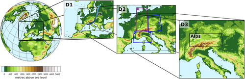
Since this tool detects all the cyclones in a given area (here we focus on Europe), the Vb cyclones need to be filtered out in a second step. The selection of Vb cyclones is done according to a method developed by Hofstätter and Chimani (2012). Hence, a box is used to define the origin over the Gulf of Genoa and one extending vertically to the east of the Alps indicating the end box. An additional box over and north of the Alps restricts the cyclones to cross the Alps as the Vb cyclone should move around the Alps. These different boxes are indicated in domain 2 in Fig. 1 as blue and violet boxes. The blue boxes labeled with ‘O’ and ‘E’ depict the origin and end box, respectively. The violet box labeled with ‘R’ marks the restriction box, where Vb cyclone passage is not allowed. These boxes ensure that the extracted tracks follow the one described by Van Bebber (1891) indicated qualitatively as blue line in domain 1 in Fig. 1. This method to identify Vb events is described in more detail by Messmer et al. (2015).

Fig. 1. The CESM output and the three nested domains (D1 to D3) with the actual topography implemented in the simulations in metres above sea level are depicted. The horizontal resolutions of D1, D2 and D3 are 27, 9 and 3 km, respectively. In D1 the typical pathway of a Vb cyclone is shown as blue line. In D2 the origin (O), end (E) and restriction (R) boxes used to extract Vb cyclones are depicted as blue and violet boxes, respectively. The box labelled ‘Alps’ in D3 denotes the area used for calculating the precipitation intensity of the Vb events.

2.4. Selection of Vb events for regional downscaling

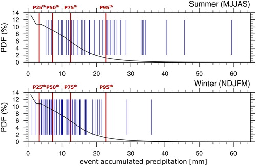
The precipitation over an Alpine box (see ‘Alps’ box in Fig. 1) is aggregated over the duration of each Vb event after detecting the Vb tracks in the global model. Hence, the large-scale and convective precipitation of the global model output are summed up to obtain total precipitation. We use total precipitation here, because a Vb cyclone does not only trigger convective precipitation (i.e. orographic lifting), but it also produces large-scale precipitation (i.e. along fronts). To avoid that precipitation from other systems than the Vb cyclone is included into this estimation we applied the following procedure: The 850 hPa geopotential height field is used to estimate the gradient around the cyclone centre in an area of 1000 × 1000 km². This gradient is then used to estimate a radius that defines a circle around the cyclone, which is considered to be influenced by it. Therefore, we first estimate the distribution of these gradients using all identified Vb cyclones. Under the assumption that stronger systems have a wider ranging influence than shallower systems, the radii are classified as follows: Gradients within plus and minus one standard deviation obtain a radius of 6°. Using a radial cap around a cyclone centre to estimate cyclone related precipitation is a widely used approach, e.g. Hawcroft et al. (2012), Zappa et al. (2013b), Yettella and Kay (2017), Booth et al. (2018) and Sinclair and Dacre (2019). Gradients that exceed (fall behind) one standard deviation, the 75th (25th) percentile or the 95th (5th) percentile of the distribution obtain a radius of 6.5° (5.5°), 7° (5°) or 7.5° (4.5°). Only the part of the Alpine box that falls within this area is used to aggregate the Vb related precipitation (for more details please refer to Messmer et al. (2015)). Additionally, the distribution of precipitation events of the typical length of Vb events during the 35 and 30 years are estimated using a bootstrapping method, which will be explained in more detail in the following. The lengths of the detected Vb events are determined for each event and in our simulations they range from 1 to 7 days in the past and from 1 to 5 days in the future (not shown). In a next step these Vb event lengths are randomly picked, making sure that a duration for a Vb event that occurs more frequent, is also selected by the randomisation more often than a duration that occurs only seldom, e.g. the shortest and longest detected period. This allows to build the distribution of precipitation in events whose duration mimics the one obtained within the simulation of Vb events. After the duration of such an event has been selected, a random date within the according period, i.e. 1979–2013 or 2070–2099, is chosen. The precipitation is then accumulated from the starting point until the length (previously picked randomly) of the event is reached. This bootstrapping procedure of randomly sampling starting dates and event length is repeated 3 million times to guarantee that the distribution of precipitation estimated is robust. Note that for the selection of the starting days, all days in the year are allowed. The probability density function is obtained and depicted as black thick line in Fig. 2. The accumulated precipitation of each event in the extended summer (MJJAS) and in the extended winter season (NDJFM) is shown as vertical blue lines in Fig. 2a and b, respectively, for the period 1979–2013 only. It becomes clear that in summer the Vb events contribute to very intense precipitation events that frequently exceed the 95th percentile. For the extended winter season, this looks differently as only few Vb events are able to trigger precipitation events exceeding the 95th percentile. The fact that only summer Vb events are able to trigger high-impact precipitation events is the main reason to select only Vb events from MJJAS. An additional reason is to avoid mixing summer and winter cyclones, as their underlying physical developing processes can be different (Ulbrich et al., 2008).

Fig. 2. Bootstrap probability density function of the accumulated precipitation from CESM data (1979–2013) in periods of time whose length mimics that of typical Vb events (black line) for extended summer (upper panel) and extended winter (lower panel). The red vertical lines indicate the 25th, 50th, 75th and 95th percentile from left to right. The vertical blue bars indicate the accumulated precipitation over the Alpine box (see Fig. 1 for the exact location of this box) of all the simulated Vb cyclones occurring during each season, respectively. The precipitation is obtained from the GCM directly.

The Vb events MJJAS are then ranked according to the event accumulated precipitation amount obtained from the GCM data for each of the two analysed periods 1979–2013 and 2070–2099 separately. The 10 events of each period that lead to the highest amounts of precipitation over the Alpine region in the global model are selected and further dynamically downscaled to analyse in more detail the physical processes of high-impact events in the past and the future.

2.5. Regional downscaling with WRF

As indicated above, a selection of the ten most precipitation intense summer Vb events for both periods, i.e. the past (1979–2013) and the future (2070–2099), are dynamically downscaled with the Weather Research and Forecasting (WRF) model. The three model domains are depicted in Fig. 1, and are 2-way nested, which allows upward communication between the different domains. The outermost and coarsest domain has a resolution of 27 km, the middle one has a resolution of 9 km and the innermost domain, covering the region of interest, has a spatial resolution of 3 km. This high resolution is needed over such a complex topography as the Alps, and furthermore allows to explicitly resolve convective processes without the need of parameterising cumulus processes (Messmer et al., 2017). All the parameterisation schemes that were used for the presented simulations are given in Table 1 in Messmer et al. (2017). The sensitivity of precipitation to the cumulus parameterisation and the domain size has been tested (not shown). This verification has been performed using real cases detected in ERA-Interim data (Dee et al., 2011), some of these cases were presented in Messmer et al. (2017). These cases were dynamically downscaled with WRF and compared to E-OBS (25 km horizontal resolution, Haylock et al. (2008)) and EURO4M-APGD (5 km horizontal resolution, Isotta et al. (2014)). The here used setting provides the best results in precipitation amounts during real Vb events. The vertical resolution used in these simulations corresponds to 50 eta levels.

The simulations are initialised 6 hours before the event starts to develop in the driving GCM. This relatively short spin-up period is selected as the Vb cyclones are very sensitive to the initialisation time (Messmer et al., 2017). This is because the Vb cyclones are triggered by a trough in the north of the Alps, therefore the position and description of this trough in the regional model is essential for it to be able to simulate such an event properly. The WRF model is adapted to climate runs in a way that the radiation scheme accounts for changes in greenhouse gases. This means, that the mixing ratios of the greenhouse gases (e.g. CO₂, N₂O, CH₄, CFC-11 and CFC-12) are adapted on a yearly basis following the protocol of the RCP8.5.

2.6. Trajectory tool HYSPLIT

Trajectories of air parcels can provide a deeper insight into the exact position of specific air parcels and provide some information on their origin. Additionally, trajectories allow to investigate atmospheric processes such as moisture uptake and loss for each of the selected air parcels. The Hybrid Single-Particle Lagrangian Integrated Trajectory (HYSPLIT) model is a complete system for computing trajectories and is able to directly digest the output from WRF (Draxler, 1999). For the present study, 48 hour backward trajectories are calculated for the Alpine region depicted in Fig. 1. Hence, the first model time step is 48 hours after the initialisation, and the last one is 36 hours later, with 3-hourly increments resulting in 13 starting points for the backward trajectories. This time period covers the main precipitation intense period during Vb events (Messmer et al., 2017). In the Alpine domain (46°–49° N and 7°–17° E) every 0.1° a trajectory is started. Thus, the area that is mostly affected by precipitation during each event is covered. For the analysis, the WRF output of domain 2 is used (Fig. 1) as the innermost is rather confined so that air parcels can exit from it within the 48 hours of the calculated trajectories. It is important to note however that because we use 2-way nesting, the solution of domain 2 is effectively the same as in domain 3 at locations where the two domains overlap. The trajectories have been calculated at different elevations: 3000, 4000, 4500, 5000, 5500, 6000, 6500, and 7000 metres above sea level, to investigate the dependency of the results from height.

3. Results

3.1. Large-scale characterisation of Vb cyclones

The 35-year time period in the past shows an occurrence of around 82.4 cyclones (counting all extratropical cyclones, not just Vb) per year on average over central Europe, whereas for the future period this number is 76.0 cyclones per year. The slight decrease can also be confirmed by the LENS where on average 106.5 cyclones per year can be detected in the past and 92.9 cyclones in the future period. This small decrease in the annual cyclone occurrence is in line with the results found by Bengtsson et al. (2006), Finnis et al. (2007), Pinto et al. (2007) and Pinto et al. (2009).

Focusing on Vb cyclones, their number shows a negative trend. 111 Vb cyclones are found in the period from 1979–2013, which corresponds to 3.2 Vb cyclones per year. This number is somewhat higher than the 82 Vb cyclones found in the ERA-Interim data set for the same period of time (Messmer et al., 2015). This might be related to the too zonal representation of the large-scale atmospheric circulation in the CESM, which tends to produce a southward displacement of the storm track in the Atlantic (Day et al., 2018; Zappa et al., 2013a). For the 30-year period in the future, the number of Vb cyclones reduces to 2.1 Vb cyclones per year (64 Vb cyclones in total). The reduction in Vb events in the future is confirmed by the LENS, showing a decrease from 2.9 Vb cyclones per year in the past to 2.6 Vb cyclones per year in the future. This decrease is consistently found throughout the 25-member subset of simulations, and is statistically significant on a 5% significance level (t-test). The reduction in the number of Vb cyclones in the future is also in line with the results by Nissen et al. (2013) who used the ECHAM5 model for their analysis. Not only the annual number of Vb cyclones is reduced, but also the summer Vb events show a trend towards a reduced occurrence, with 1.2 and 0.7 Vb cyclones per year on average in the seamless simulation during MJJAS in the past and future, respectively.

The reduced number of Vb cyclones is related to a shift in the cyclone path between the past and the future period. To assess this, the frequency of all cyclones and Vb cyclones and their possible changes are studied (Figs. 3–5). The cyclone frequency is calculated using the radius calculated by the tracking tool described in Section 2.3. To estimate the cyclone frequency, every grid point within the area framed by the radius around the cyclone centre is considered as one, while the surrounding grid points are considered as zero. All these areas are estimated for each cyclone centre and for every time step within one year. All these circles are then accumulated and normalized by the number of time steps within one year. Hence, the cyclone frequency indicates the yearly probability of a certain grid point to be influenced by an extratropical cyclone. Although the total cyclone number only slightly changes between the two periods, a change in the cyclone tracks is still observable in Fig. 3. It becomes clear that cyclone frequency is reduced over almost entire Europe in the future, including also the passage over the Mediterranean Sea and east of the Alps, which are both important regions for the passage of Vb cyclones (Fig. 3c). This general reduction over Europe and the Mediterranean is confirmed by the LENS with significance (at the 5% level; Fig. 3f). The reduction over the Mediterranean Sea is also in line with findings of Lionello et al. (2008). Additionally, an increase in cyclone frequency over Scandinavia is found for the seamless simulations, while the LENS simulation shows a more pronounced increase in cyclone frequency over Iceland. The cyclone frequency pattern thus indicates mainly a northward shift of the storm track as the frequency over the British Isles is highest in the past and is moved more to Scandinavia and higher north. Note that the additional eastward shift observed in the seamless simulation, might just reflect internal variability. Overall, the northward shift in storm track of LENS and the seamless simulation agrees with findings of Nissen et al. (2013).

Fig. 3. Annual cyclone frequency of all detected cyclone centres (not only Vb cyclones) for the seamless CESM run and the period 1979–2013 (a), 2070–2099 (b) and the difference between (b) and (a) in (c). (d) and (e) show the annual cyclone frequency of all detected cyclones for the LENS for the period 1990–2005 and 2071–2080, respectively. (f) shows the difference between (e) and (d). The hatched area shows significant changes using a non-parametric Mann-Whitney-U test on a 10% and 5% level for (c) and (f), respectively. The grey area indicates places, where the topography exceeds 1000 meters above sea level.

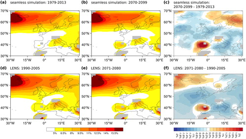
Fig. 4. Annual cyclone frequency of cyclones that pass through the origin box, labeled with ‘O’. The other two boxes indicate the end box (‘E’) and the restriction box (‘R’). (a) and (b) depict the frequency obtained from the seamless CESM run in the period 1979–2013 and 2070–2099, respectively. (c) shows the difference between (b) and (a). (d) and (e) illustrate the frequency of the LENS for the periods 1990–2005 and 2071–2080, respectively. (f) shows the difference between (e) and (d). The hatched area indicates significant changes on a 10% and 5% significance level, for (c) and (f), respectively, using the nonparametric Mann-Whitney-U test. The grey area indicates places, where the topography exceeds 1000 meters above sea level.

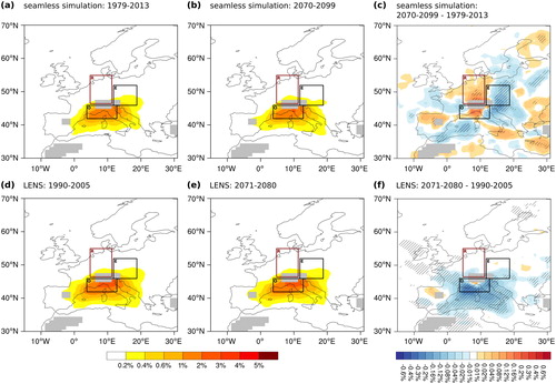
Fig. 5. The mean annual Vb cyclone frequency of the seamless CESM simulation for the period 1979–2013 (a) and 2070–2099 (b) and (c) showing the difference between (b) and (a). (d) and (e) show the same, but for the LENS and the period 1990–2005 and 2071–2080, respectively. (f) indicates the difference between (e) and (d). The hatched area indicates significant changes on a 10% and 5% significance level, for (c) and (f), respectively, using the nonparametric Mann-Whitney-U test. The grey area indicates places, where the topography exceeds 1000 meters above sea level.

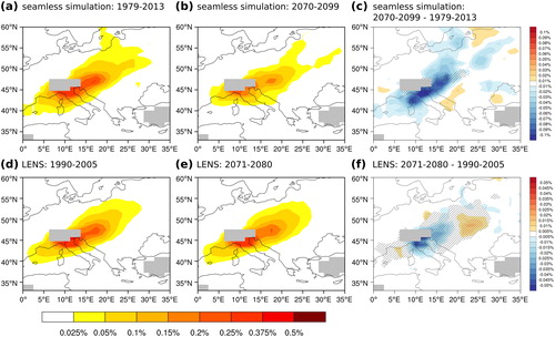
The analysis of the fraction between the cyclones that fulfill the first criterion of being present in the origin box (‘O’-labelled box in Fig. 4) at the beginning of the cyclones lifetime and the ones that can be eventually classified as Vb cyclones, i.e. pass also through the end box (‘E’-labelled box in Fig. 4) without crossing the Alps (‘R’-labelled box in Fig. 4), helps to understand why the number of Vb cyclones is reduced in the future. For the years between 1979 and 2013, an annual average number of 18.1 cyclones is detected in the origin box, whereas only 3.2 Vb cyclones per year on average develop out of these, as mentioned above. This indicates that 17.7% of the cyclones that pass through the origin box follow the pathway described by Van Bebber (1891). In the future period, 17.1 cyclones are detected on average per year in the origin box. Nevertheless, only 2.1 cyclones per year are Vb cyclones in the period 2070–2099. This means that only 12.3% of the cyclones passing through the origin box are able to develop a Vb cyclone. The differences in cyclone frequency shown in Fig. 4c indicate that there is a reduction in cyclone passage on the eastern flanks of the Alps as well as over the western Mediterranean. This can also be confirmed by the LENS simulations. In the LENS there is an even stronger reduction detectable over the whole typical Vb passage, i.e. the Ligurian Sea and in the Adriatic Sea in the future. These two areas are actually important for the passage of Vb cyclones which lead to the reduction in Vb cyclones in a warmer climate. The increase on the northern side of the Alps in the seamless simulation (Fig. 4c) is only induced by changes of very few cyclone tracks in the future climate, as illustrated by a very low cyclone frequency (Fig. 4a, b). Hence, this signal is not of major importance and certainly is induced by internal variability due to the use of a single simulation.

Although a reduction in the Vb cyclone occurrence is detected, the cyclone frequency reveals very similar patterns for the Vb events in the two periods, as Fig. 5a, b show. This is mainly ascribed to the way Vb cyclones are defined. The high probability spots are located at nearly the same location. This is not only true for the seamless simulation (Fig. 5a–c), but also for the LENS (Fig. 5d–f). Even though the patterns are very similar, still a slight eastward shift is found in the future compared to the past. The tracks obtained from the ensemble show that the frequency close to the Alps is reduced and that the tracks of the Vb cyclones seem to extend more to the east instead of northward.

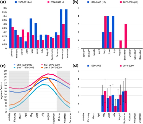
The annual distribution of all Vb cyclones again shows similar behaviour (Fig. 6a). In both periods, there are fewer Vb events in the summer season than in winter. In the future, the number of cyclones in May and June is much lower compared to the past simulation in the summer season. December events are noticeably rare in the future simulation compared to the past one, although this may be due to the effect of having less Vb cyclones tracked in the future period.

Fig. 6. (a) the mean annual number of Vb cyclones per month in the period between 1979–2013 (blue bars) and 2070–2099 (red bars) during the respective months (x-axis). (b) The distribution of the 10 heavy precipitation summer Vb events of both periods. (c) monthly average Mediterranean sea surface temperature (SST) and European 2-m temperature (2-m T) of the past period (blue lines) and the future period (red lines). The grey shaded area covers the months of the year that do not belong to the analysed extended summer season (MJJAS). (d) the mean monthly distribution of the 10 heavy precipitation summer Vb events found in the LENS for the periods 1990–2005 (blue bars) and 2071–2080 (red bars). The black lines indicate ± one standard deviation.

3.2. Large-scale characteristics of extreme Vb events

To gain further insights in Vb cyclones we focus on the 10 heaviest precipitation summer Vb events of each period. Comparing first the spatial distribution of cyclone frequency we find almost no changes between the past and the future period (therefore not shown). Also the lifetime and the central pressure only show insignificant changes. Thus, extreme Vb cyclones remain unchanged with respect to lifetime and central pressure and seem to move on similar tracks with more or less equal latitudinal extent during their mature and precipitation intense stage.

Besides this overall agreement, there are changes in the monthly occurrence of the extreme Vb cyclones (Fig. 6b). While in the period from 1979–2013 the Vb cyclones predominantly occur in June and July, in the future period the extreme events mainly are found in the edge months May and September. To be able to test if this is just a feature of our seamless simulation, we also assess extreme Vb cyclones in the LENS. Since the number of years obtained from the LENS is much smaller than the one we used from the seamless simulation, we applied the following approach: from the 25 ensemble simulations with 16 (10) years in the past (future) there are in total 317 (224) years where Vb cyclones can be detected at all. From this total number of years, 35 (30) years in the past (future) are selected randomly. From these 35 (30) the 10 most heavy precipitation Vb events are selected and the month of their appearance is recorded. This procedure is repeated 317 − 35 = 282 (224 − 30 = 194) times. The resulting distribution (Fig. 6d) shows that extreme Vb cyclones experience a substantial reduction in July, which is compensated by increases in the other months, especially May and August, in the future.

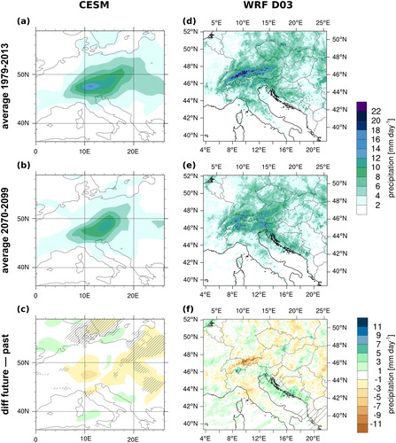
To gain more details of the impact of these extreme Vb cyclones, the precipitation patterns of the 10 most heavy precipitation Vb events is presented for both periods (Fig. 7a, b). Precipitation over southern Germany, Switzerland and western Austria is highest, although also Poland and the Czech Republic are affected by heavy precipitation in the period 1979 to 2013. This precipitation pattern resembles the one obtained with ERA-Interim for the past period (Fig. 5 (left panel) in Messmer et al., 2015), which also shows a peak precipitation north of the Alpine ridge and additionally enhanced precipitation over Poland, southern Germany and the Czech Republic. The precipitation pattern for the future period (Fig. 7b) illustrates a reduction over the Alpine area and thus, a shift of the peak precipitation to the east. Furthermore, the precipitation associated with extreme Vb cyclones is slightly increased over the eastern Adriatic coast for the future period, though not significant (Fig. 7). Since the 10 future tracks do not imply a southward shift compared to the past ones, this change in precipitation is not related to a more southern position of the average future heavy precipitation summer Vb event. In order to further evaluate the possible reason for this change in precipitation, these extreme events for both periods are analysed in more detail from the regional model perspective, described in the following subsection.

Fig. 7. Average daily precipitation of the 10 most intense precipitation summer Vb events for the CESM (left column) and WRF (right column) output for the period 1979–2013 (a and d) and 2070–2099 (b and e). (c) and (f) depict differences between (b) and (a) and (e) and (d), respectively. Shading indicates precipitation in mm day⁻¹. Hatched areas indicate significant changes using the non-parametric Mann-Whitney-U test and a significance level α = 10%.

3.3. Regional scale processes

The downscaling of the 10 Vb events in both periods allows to investigate the processes that take place during these events. To get an impression of the processes involved in the 10 heavy precipitation summer Vb cyclones, composites of different variables are analysed for each period, separately. Thereby we compared the precipitation during the extreme events with moisture fluxes from the land and the ocean to separate between land- and ocean-induced processes. Temperature changes are used to assess thermodynamic processes involved in changing extreme Vb cyclones in the future. In doing so, Fig. 8 depicts the spatial average of the ensemble mean of several variables for the 10 heavy precipitation summer Vb events in the two different periods, which are spatially and temporally averaged. In most panels the spatial average is calculated for domain 3, since this domain fully covers the area that is influenced by the Vb cyclone (compare Fig. 1 for the exact area of this domain) although results for the Alpine region are also shown (compare Alp box in Fig. 1).

Fig. 8. The panels show the mean over 10 Vb events for the period between 1979–2013 (blue bar) and 2070–2099 (red bar). The depicted variables are (a) mean daily precipitation [mm], (b) mean daily upward moisture flux over land [kg m⁻²day⁻¹], (c) mean daily upward moisture flux over the ocean [kg m⁻²day⁻¹], (d) precipitable water [kg m⁻²], (e) mean daily precipitation over the Alps [mm], (f) mean daily sea surface temperature [° C], (g) mean daily air temperature at 850 hPa [° C], and (h) mean daily 2-m air temperature [° C]. All panels except for (e) show a spatial mean over domain 3, whereas (e) shows a spatial mean over the Alpine box. Asterisks located over the red bars indicate that the future values are significantly different from the past ones using the non-parametric Mann-Whitney-U test and a significance level α = 10%. The black vertical bar indicates ± one standard deviation across the 10 events.

Figure 8a depicts the mean daily precipitation for the past (blue bar) and the future period (red bar), respectively. The results of the average precipitation show that precipitation amounts exhibit hardly any change over domain 3 comparing the past and the future. This result is not clear from the precipitation pattern presented in Fig. 7, as from the pattern alone it seems that in the future the precipitation is generally smaller than in the past. Also the inter-case standard deviations of the 10 events (indicated with the black line) exhibit a similar range for both periods. Nevertheless, there are changes observable in the moisture supply of the atmospheric moisture content. There is a significant decrease in moisture delivery to the atmosphere from the land, and hence from the moisture contained in the soil in the future (Fig. 8b). This is related to a draining of the soil in the future period. The soil water content averaged over the whole domain 3 and over the whole event period of the first and most weather relevant soil layer in the 10 analysed Vb events reduces from 0.268 m³ m⁻³ to 0.251 m³ m⁻³. However, the land is not the only source of moisture for the atmosphere, as also the ocean can contribute to atmospheric moisture content. Indeed, in the future the ocean has a more important role in supplying the atmosphere with moisture than in the past period (Fig. 8c). This is due to the increase in sea surface temperature of 2 K on average from the past to the future indicated in Figs. 6c and 8f. All in all, the changes in the upward moisture flux over land and the ocean tend to compensate each other, and lead to a small increase in the vertically integrated total moisture, i.e. precipitable water (Fig. 8d). The increase in precipitable water from 23.3 to 24.8 kg m⁻² corresponds to around 6%. This small increase in precipitable water is explained by the Clausius-Clapeyron relationship. Hence, on average the air temperature over land is increased by about 1 K on different elevations as Fig. 8g and 8h reveal. Thus, the 1 K temperature increase at 2-m and 850 hPa, which describe levels that also contribute to the largest share in moisture amounts in the atmosphere, can explain the increase of around 6% in the precipitable water. The different rate of change in 2-m and 850 hPa temperature, i.e. 1 K and the SSTs, i.e. 2 K, between the two different time periods indicate a stronger temperature gradient at the coastal areas for the period from 2070–2099. Such a change in the temperature gradient can induce a change in precipitation patterns, which will be investigated in more detail below.

There seems to be not much difference in the precipitation amounts aggregated over the whole domain 3 between the past and the future. Nevertheless, there are regional differences that become clear when focusing on the Alps (Fig. 8e). Hence, the averaged precipitation over the Alpine region indicates a significant reduction in the future compared to the past. To investigate this issue in more detail, Fig. 7d and 7e show the spatial distribution of the precipitation patterns of the two periods. It becomes clear that the precipitation amounts in the Alpine region, and especially over western Austria, become strongly reduced under future climate conditions, which qualitatively agrees with the result obtained with the CESM. When also considering the difference plot in Fig. 7f, further changes are revealed. A remarkable difference between the Vb events in the past and the future is an increase in precipitation over the Adriatic coast. This effect was described by Messmer et al. (2017), and is related to the increased temperature gradient between land and sea mentioned in the previous paragraph. The stronger warming of the SSTs, compared to the low level air temperature shown in Fig. 8f–h lead to an increase in this gradient in the future, which results in lifting of the warmer air masses from the sea over the colder ones over land. Furthermore, the Dinaric Alps, which are located at the Adriatic coast, further contribute to the lifting of slightly more moist air parcels in the future. All this lifting leads to precipitation along the coastal area of the east Adriatic Sea. These results are in good agreement with the ones presented by Volosciuk et al. (2016) and Messmer et al. (2017), which obtained similar changes in precipitation patterns through a series of sensitivity studies with the Mediterranean sea surface temperatures. Note that we have performed this analysis for different numbers of Vb events in the past and the future (i.e. 20, 15 and 10 past versus 10, 10 and 5 future events, respectively). This has been done to account for the fact that in the future less Vb cyclones can be detected and by comparing 10 versus 10 events the future period might include less extreme events. The tests show that the selection of the number of events has no effect on the precipitation patterns that are presented here.

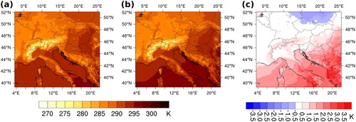
Figure 9 provides further insight on the 2-m temperature. Compared to the past period (Fig. 9a), there is a warming of the Mediterranean Sea observable for the 10 heavy precipitation events in the future climate projection (Fig. 9b), whereas the warming over land is not everywhere obvious. The southern part of the domain becomes warmer than in the past period. The 10 Vb events occurring in the future period are shifted to the colder seasons compared to the past simulation, where the average temperature is equally warm or slightly warmer compared to the highest mean temperature in the past simulation, i.e. July (only the future May temperature is colder than the past July temperature; Fig. 6c). The Mediterranean Sea shows the expected stronger warming than the costal areas, supporting the aforementioned increase in temperature gradient that invokes precipitation in these regions (Fig. 6c). The changes in 2-m temperature do not reveal statistical significance at the 5% level, which further indicates that temperatures are rather similar during these events. The similar temperature conditions in the present and the future climate cases indicate that heavy precipitation Vb events preferably occur during specific temperature conditions. These temperature conditions seem to be more often fulfilled in the high summer season in the past period, while in the future period these are more often obtained in the colder months of MJJAS. The negligible difference in 2-m temperature over land further supports the results found through the sensitivity studies performed by Volosciuk et al. (2016) and Messmer et al. (2017). Hence, the sensitivity studies, where only sea surface temperatures are changed, but not the land surface temperature, can be argued to have provided a good approximation for the more realistic results obtained here.

Fig. 9. Average daily 2-m temperature of the 10 most intense precipitation summer Vb events for the domain 3 of the WRF simulations for the period 1979–2013 (a) and 2070–2099 (b). (c) depicts the differences between (b) and (a). Shading indicates the temperature in K. No statistical significance can be found on a 5% level.

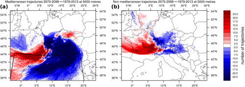
Finally, Fig. 10 shows the difference in the backward trajectories that are obtained for the 10 heavy precipitation summer Vb events with a starting elevation of 5000 m in the Alpine box. Figure 10a shows the trajectories that come from the Mediterranean region (36.5–44.5° N and 3.5–20° E), while Fig. 10b shows the trajectories that never pass the Mediterranean Sea. The trajectory analysis reinforces the finding that most of the air during Vb events comes from the Mediterranean region and hence, from the south towards the northern side of the Alps, rather than directly from the north, as it is expected during Vb events (Messmer et al., 2017) (not shown). Note that this is true for both periods. Nevertheless, in the future period trajectories avoid the Mediterranean Sea more frequently, and thus directly travel to the northern side of the Alps. Furthermore, it seems that in the future the air parcels take a more zonal direction towards the Alps from the Mediterranean Sea, while in the past period the trajectories are more circular around the eastern flanks of the Alps. Note that the changes between the trajectories show almost everywhere statistical significance using the non-parametric Mann-Whitney-U test and a significance level α = 10% (not shown). These results are consistent for all the starting elevations described in Section 2.6 (not shown).

Fig. 10. Shading indicates the differences in the location of the 48-hour backward trajectories between averages of the 10 events of the period 2070–2099 and 1979–2013. Note that different trajectories can pass a certain point several times. The difference indicates a reduced or increased air parcel passage. The starting position is at 5000 m. (a) shows all the trajectories that pass through the Mediterranean region (black box), while (b) shows the trajectories that do not pass through the Mediterranean region.

4. Summary and outlook

The present study aims at investigating the sensitivity of Vb cyclones to climate change. To detect changes in Vb cyclones induced by climate change, the years 1979–2013 and 2070–2099 of a transient climate simulation with the CESM model and the large CESM ensemble for the periods 1990–2005 and 2071–2080 (Kay et al., 2015) are analysed in more detail. A special focus is put on the 10 most intense precipitation events in MJJAS of both the past and the future period of the transient climate simulation by dynamically downscaling these events with WRF.

The analysis of the global model simulation shows that over Central Europe an annual cyclone occurrence of 106.5 (82.4) can be found in the LENS (seamless simulation) in the past and 92.9 (76.0) cyclones can be identified in the future. Both simulations show a slight reduction in annual cyclone occurrence in the future, which is in line with previous studies (Bengtsson et al., 2006; Finnis et al., 2007; Pinto et al., 2007, 2009). Although the changes in total cyclone occurrence do not show substantial changes for the future period, there is a clearer trend in Vb cyclones. Thereby, 2.9 (3.2) Vb cyclones per year are detected in the LENS (seamless simulation) for the past period, whereas for the future period only 2.6 (2.1) Vb cyclones per year are tracked in the LENS (seamless simulation). The reduction in the Vb events is consistent throughout the LENS members and is significant on a 5% significance level.

The distribution of trajectories reveals that the reduction in Vb events in the future is connected to changes in the cyclone track, as stated by Nissen et al. (2013). Precisely, the difference in cyclone frequency between the past and the future for all European cyclones demonstrates a slight northward shift, as there is a strong reduction over the British Islands and Central Europe and an increase over Iceland in the LENS and Scandinavia in the seamless simulation in the future. The slight eastward shift in the seamless simulation is mainly a result of the internal variability. Furthermore, the cyclones that pass through the origin box, i.e. the first criterion to be classified as Vb cyclone, show a reduction in cyclone frequency over the Mediterranean Sea and east of the Alps in the future climate in the seamless and LENS simulation, which are both important regions for Vb cyclone passage. Such a reduction over the Mediterranean Sea is in line with Lionello et al. (2008).

Still, the Vb cyclones that are detected in both periods show similar trajectories. There is a subtle eastward shift observable in the cyclone frequency. Similarly, the cyclone dynamics hardly differ across the 10 heavy precipitation summer Vb cyclones in both periods. The monthly distribution of these 10 events of each period shows some divergences. In the past period, the Vb events occur in May, June, and July, while in the future period such events are favoured in May, June, August and September. This shift towards the colder months in the summer season is found in the LENS and the seamless simulation, respectively.

The dynamical downscaling of the 10 events demonstrates that changes in the thermodynamics occur during such high impact summer Vb events: Moisture is mostly supplied by the moisture flux over the ocean, as this is increased in the future climate simulations, and this is accompanied by a significant reduction in the moisture flux over the soil. This is mainly because of a drying of the soil and a heating of the Mediterranean Sea. These changes in moisture supply compensate each other to a great extent, and therefore have only a minor effect on the net available atmospheric moisture, which shows an increase of around 6% in the future cases. This increase is explained by the Clausius-Clapeyron scaling, driven by an average warming of around 1 K in the lower troposphere. Although there exist little change in the precipitation amounts over central Europe, a shift in precipitation patterns becomes evident: A reduction in precipitation is found over the Alps together with an increase over the east Adriatic coast in the future. This change in precipitation pattern corresponds well with the Mediterranean SST sensitivity studies described by Volosciuk et al. (2016) and Messmer et al. (2017). Furthermore, this region hosts the Dinaric Alps, which lead to a lifting of warmer and more moist air, promoting convective precipitation in this region. The differences in the temperature field between the 10 events in the past and in the future reveal the following results: The north of the Alps is slightly colder in the future than in the past, while around and south of the Alps almost no warming is found. Only in southern Europe a warming is detected. This suggests that Vb events that lead to heavy precipitation need temperature conditions that are more frequently met in the warmer summer months in past climate and in the colder summer months in the future, being an additional reason for the reduction in summer Vb cyclones in the future. Furthermore, the contrast between almost no warming over land and a heating of the SSTs at the coast increases the instability at the coastal areas, leading to more precipitation events there. Finally, the trajectory analysis reveals a more zonal behaviour of the 10 future Vb events, again explaining the increase (decrease) of precipitation over the Balkan coast (Alps).

To strengthen these results, it would be desirable to perform this study with different general circulation models, as one caveat of this study is that the analysis is based on just one model. Although the CESM model is considered a state-of-the-art model, it generally suffers from too zonal winds in the mid-latitudes related to systematic biases in the geopotential height field, which is a problem known in almost all CMIP5 models (Davini and D’Andrea, 2016). It is unknown how this bias of the CESM influences the ability to track and represent Vb events. Hence, repeating the experiments with other general circulation models (e.g. model output of Climate Model Intercomparison Project (CMIP6), with 6-hourly temporal resolution) and different climate change scenarios would strongly increase the confidence in the results presented here, as well as offer the opportunity to quantify the uncertainty associated with them.

Acknowledgments

The simulations are all run at the Swiss National Supercomputing Centre CSCS. The ERA-Interim reanalysis data were provided by the ECMWF. We also acknowledge Sandro Blumer for making available the CESM output, which provides the initial and 6-hourly boundary conditions for the RCM. We are also thankful for the helpful comments of the two anonymous reviewers, which significantly improved the manuscript.

Additional information

Funding

The authors are thankful for the funding provided by the Dr. Alfred Bretscher-Fonds für Klima- und Luftverschmutzungsforschung. Thanks are also due to the support provided by the Oeschger Centre for Climate Change Research and the Mobiliar lab for climate risks and natural hazards (Mobilab). MM is thankful for the support provided by the Swiss National Science Foundation (project P2BEP2_181837). JJGN acknowledges the CARM for the funding provided both through the Seneca Foundation (project 20640/JLI/18), as well as the “Juan de la Cierva-Incorporación” program (IJCI-2015-26914).

References

- Bengtsson, L., Hodges, K. I. and Keenlyside, N. 2009. Will extratropical storms intensify in a warmer climate? J. Clim. 22, 2276–2301. doi:10.1175/2008JCLI2678.1
- Bengtsson, L., Hodges, K. I. and Roeckner, E. 2006. Storm tracks and climate change. J. Clim. 19, 3518–3543. doi:10.1175/JCLI3815.1
- Beniston, M., Stephenson, D. B., Christensen, O. B., Ferro, C. A. T., Frei, C. and co-authors. 2007. Future extreme events in European climate: an exploration of regional climate model projections. Clim. Change 81, 71–95. doi:10.1007/s10584-006-9226-z
- Blender, R., Fraedrich, K. and Lunkeit, F. 1997. Identification of cyclone-track regimes in the North Atlantic. QJ. Royal Met. Soc. 123, 727–741. doi:10.1002/qj.49712353910
- Booth, J. F., Naud, C. M. and Jeyaratnam, J. 2018. Extratropical cyclone precipitation life cycles: a satellite-based analysis. Geophys. Res. Lett. 45, 8647–8654. doi:10.1029/2018GL078977
- Catto, J. L., Shaffrey, L. C. and Hodges, K. I. 2011. Northern Hemisphere extratropical cyclones in a warming climate in the HiGEM high-resolution climate model. J. Clim. 24, 5336–5352. doi:10.1175/2011JCLI4181.1
- Chikamoto, M. O., Timmermann, A., Yoshimori, M., Lehner, F., Laurian, A. and co-authors. 2016. Intensification of tropical Pacific biological productivity due to volcanic eruptions. Geophys. Res. Lett. 43, 1184–1192. doi:10.1002/2015GL067359
- Davini, P. and D’Andrea, F. 2016. Northern Hemisphere atmospheric blocking representation in global climate models: twenty years of improvements? J. Clim. 29, 8823–8840. doi:10.1175/JCLI-D-16-0242.1
- Day, J. J., Holland, M. M. and Hodges, K. I. 2018. Seasonal differences in the response of Arctic cyclones to climate change in CESM1. Clim. Dyn. 50, 3885–3903. doi:10.1007/s00382-017-3767-x
- Dee, D. P., Uppala, S. M., Simmons, A. J., Berrisford, P., Poli, P. and co-authors. 2011. The ERA-interim reanalysis: configuration and performance of the data assimilation system. QJR Meteorol. Soc. 137, 553–597. doi:10.1002/qj.828
- Draxler, R. R. 1999., HYSPLIT Radiological Transport and Dispersion Model Implementation on NCEP Cray. U.S. Department of Commerce, National Oceanic and Atmospheric Administration, National Weather Service, Office of Meteorology, Science Division, Silver Spring, Maryland. Technical Procedures Bulletin; no. 458.
- Easterling, D. R., Evans, J. L., Groisman, P. Y., Karl, T. R., Kunkel, K. E. and co-authors. 2000. Observed variability and trends in extreme climate events: A brief review. Bull. Amer. Meteor. Soc. 81, 417–425. doi:10.1175/1520-0477(2000)081<0417:OVATIE>2.3.CO;2
- Finnis, J., Holland, M. M., Serreze, M. C. and Cassano, J. J. 2007. Response of Northern Hemisphere extratropical cyclone activity and associated precipitation to climate change, as represented by the community climate system model. J. Geophys. Res. 112, G04S42.
- Gulev, S. K., Zolina, O. and Grigoriev, S. 2001. Extratropical cyclone variability in the Northern Hemisphere winter from the NCEP/NCAR reanalysis data. Clim. Dyn. 17, 795–809. doi:10.1007/s003820000145
- Hawcroft, M. K., Shaffrey, L. C., Hodges, K. I. and Dacre, H. F. 2012. How much Northern Hemisphere precipitation is associated with extratropical cyclones? Geophys. Res. Lett. 39, 1–7.
- Haylock, M. R., Hofstra, N., Klein Tank, A. M. G., Klok, E. J., Jones, P. D. and co-authors. 2008. A European daily high-resolution gridded data set of surface temperature and precipitation for 1950–2006. J. Geophys. Res. 113, D20119. doi:10.1029/2008JD010201
- Hoegh-Guldberg, O., Jacob, D., Taylor, M., Bindi, M., Brown, S. and co-authors. 2018. Impacts of 1.5 °C of global warming on natural and human systems. In: Global Warming of 1.5 °C. An IPCC Special Report on the Impacts of Global Warming of 1.5 °C above Pre-Industrial Levels and Related Global Greenhouse Gas Emission Pathways, in the Context of Strengthening the Global Response to the Threat of Climate Change, Sustainable Development, and Efforts to Eradicate Poverty [Masson-Delmotte, V., P. Zhai, H.-O. Pörtner, D. Roberts, J. Skea, P.R. Shukla, A. Pirani, W. Moufouma-Okia, C. Péan, R. Pidcock, S. Connors, J.B.R. Matthews, Y. Chen, X. Zhou, M.I. Gomis, E. Lonnoy, T. Maycock, M. Tignor, and T. Waterfield (eds.)]. In Press.
- Meehl, G. A., Washington, W. M., Arblaster, J. M., Hu, A., Teng, H. and co-authors. 2013. Climate Change Projections in CESM1(CAM5) Compared to CCSM4. J. Clim. 26, 6287–6308. doi:10.1175/JCLI-D-12-00572.1
- Hofstätter, M. and Chimani, B. 2012. Van Bebber’s cyclone tracks at 700 hPa in the Eastern Alps for 1961–2002 and their comparison to circulation type classifications. Metz. 21, 459–473. doi:10.1127/0941-2948/2012/0473
- Hurrell, J. W., Holland, M. M., Gent, P. R., Ghan, S., Kay, J. E. and co-authors. 2013. The Community Earth System Model: a framework for collaborative research. Bull. Amer. Meteor. Soc. 94, 1339–1360. doi:10.1175/BAMS-D-12-00121.1
- IPCC. 2013. Climate change 2013: the physical science basis. In: Contribution of Working Group I to the Fifth Assessment Report of the Intergovernmental Panel on Climate Change [Stocker, T.F., D. Qin, G.-K. Plattner, M. Tignor, S.K. Allen, J. Boschung, A. Nauels, Y. Xia, V. Bex and P.M. Midgley (eds.)]. Cambridge University Press, Cambridge, UK, and New York, NY, USA, 1535 pp.
- Isotta, F. A., Frei, C., Weilguni, V., Percec Tadić, M., Lassègues, P. and co-authors. 2014. The climate of daily precipitation in the Alps: development and analysis of a high-resolution grid dataset from pan-Alpine rain-gauge data. Int. J. Climatol. 34, 1657–1675. doi:10.1002/joc.3794
- Kay, J. E., Deser, C., Phillips, A., Mai, A., Hannay, C. and co-authors. 2015. The Community Earth System Model (CESM) large ensemble project: a community resource for studying climate change in the presence of internal climate variability. Bull. Amer. Meteor. Soc. 96, 1333–1349. doi:10.1175/BAMS-D-13-00255.1
- Leckebusch, G. C. and Ulbrich, U. 2004. On the relationship between cyclones and extreme windstorm events over Europe under climate change. Global Planet. Change 44, 181–193. doi:10.1016/j.gloplacha.2004.06.011
- Lehner, F., Joos, F., Raible, C. C., Mignot, J., Born, A. and co-authors. 2015. Climate and carbon cycle dynamics in a CESM simulation from 850 to 2100 CE. Earth Syst. Dynam. 6, 411–434. doi:10.5194/esd-6-411-2015
- Lionello, P., Boldrin, U. and Giorgi, F. 2008. Future changes in cyclone climatology over Europe as inferred from a regional climate simulation. Clim. Dyn. 30, 657–671. doi:10.1007/s00382-007-0315-0
- Lionello, P., Dalan, F. and Elvini, E. 2002. Cyclones in the Mediterranean region: the present and the doubled CO2 climate scenarios. Clim. Res. 22, 147–159. doi:10.3354/cr022147
- Löptien, U., Zolina, O., Gulev, S., Latif, M. and Soloviov, V. 2008. Cyclone life cycle characteristics over the Northern Hemisphere in coupled GCMs. Clim. Dyn. 31, 507–532. doi:10.1007/s00382-007-0355-5
- Messmer, M., Gómez-Navarro, J. J. and Raible, C. C. 2015. Climatology of Vb cyclones, physical mechanisms and their impact on extreme precipitation over Central Europe. Earth Syst. Dynam. 6, 541–553. doi:10.5194/esd-6-541-2015
- Messmer, M., Gómez-Navarro, J. J. and Raible, C. C. 2017. Sensitivity experiments on the response of Vb cyclones to sea surface temperature and soil moisture changes. Earth Syst. Dynam. 8, 477–493. doi:10.5194/esd-8-477-2017
- MeteoSchweiz. 2006. Starkniederschlagsereignis August 2005. Arbeitsberichte Der MeteoSchweiz 211, 63. pp.
- Muskulus, M. and Jacob, D. 2005. Tracking cyclones in regional model data: The future of Mediterranean storms. Adv. Geosci. 2, 13–19. doi:10.5194/adgeo-2-13-2005
- Neale, R. B., Richter, J. H., Conley, A. J., Park, S., Lauritzen, P. H. and co-authors. 2010. Description of the NCAR Community Atmosphere Model (CAM 4.0). Technical report, National Center for Atmospheric Research (NCAR). 212 pp.
- Nied, M., Pardowitz, T., Nissen, K., Ulbrich, U., Hundecha, Y. and co-authors. 2014. On the relationship between hydro-meteorological patterns and flood types. J. Hydrol. 519, (Part D), 3249–3262. doi:10.1016/j.jhydrol.2014.09.089
- Nissen, K. M., Leckebusch, G. C., Pinto, J. G. and Ulbrich, U. 2014. Mediterranean cyclones and windstorms in a changing climate. Reg. Environ. Change 14, 1873–1890. doi:10.1007/s10113-012-0400-8
- Nissen, K. M., Ulbrich, U. and Leckebusch, G. C. 2013. Vb cyclones and associated rainfall extremes over Central Europe under present day and climate change conditions. Metz. 22, 649–660. doi:10.1127/0941-2948/2013/0514
- Pinto, J. G., Spangehl, T., Ulbrich, U. and Speth, P. 2006. Assessment of winter cyclone activity in a transient ECHAM4-OPYC3 GHG experiment. Metz. 15, 279–291. doi:10.1127/0941-2948/2006/0128
- Pinto, J. G., Ulbrich, U., Leckebusch, G. C., Spangehl, T., Reyers, M. and co-authors. 2007. Changes in storm track and cyclone activity in three SRES ensemble experiments with the ECHAM5/MPI-OM1 GCM. Clim. Dyn. 29, 195–210. doi:10.1007/s00382-007-0230-4
- Pinto, J. G., Zacharias, S., Fink, A. H., Leckebusch, G. C. and Ulbrich, U. 2009. Factors contributing to the development of extreme North Atlantic cyclones and their relationship with the NAO. Clim. Dyn. 32, 711–737. doi:10.1007/s00382-008-0396-4
- Raible, C. C., Della-Marta, P. M., Schwierz, C., Wernli, H. and Blender, R. 2008. Northern Hemisphere extratropical cyclones: A comparison of detection and tracking methods and different reanalyses. Mon. Wea. Rev. 136, 880–897. doi:10.1175/2007MWR2143.1
- Raible, C. C., Messmer, M., Lehner, F., Stocker, T. F. and Blender, R. 2018. Extratropical cyclone statistics during the last millennium and the 21st century. Clim. Past 14, 1499–1514. doi:10.5194/cp-14-1499-2018
- Raible, C. C., Ziv, B., Saaroni, H. and Wild, M. 2010. Winter synoptic-scale variability over the Mediterranean Basin under future climate conditions as simulated by the ECHAM5. Clim. Dyn. 35, 473–488. doi:10.1007/s00382-009-0678-5
- Schneidereit, A., Blender, R. and Fraedrich, K. 2010. A radius–depth model for midlatitude cyclones in reanalysis data and simulations. QJR Meteorol. Soc. 136, 50–60. doi:10.1002/qj.523
- Seneviratne, S. I., Nicholls, N., Easterling, D., Goodess, C. M., Kanae, S. and co-authors. 2012. Changes in climate extremes and their impacts on the natural physical environment. In: Managing the Risks of Extreme Events and Disasters to Advance Climate Change Adaptation [Field, C.B., V. Barros, T.F. Stocker, D. Qin, D.J. Dokken, K.L. Ebi, M.D. Mastrandrea, K.J. Mach, G.-K. Plattner, S.K. Allen, M. Tignor, and P.M. Midgley (eds.)]. A Special Report of Working Groups I and II of the Intergovernmental Panel on Climate Change (IPCC). Cambridge University Press, Cambridge, UK, and New York, NY, USA, pp. 109–230.
- Sickmöller, M., Blender, R. and Fraedrich, K. 2000. Observed winter cyclone tracks in the Northern Hemisphere in re-analysed ECMWF data. QJR Meteorol. Soc. 126, 591–620. doi:10.1002/qj.49712656311
- Sinclair, V. A. and Dacre, H. F. 2019. Which extratropical cyclones contribute most to the transport of moisture in the Southern Hemisphere? J. Geophys. Res. Atmos. 124, 2525–2545. doi:10.1029/2018JD028766
- Trigo, I. F. 2006. Climatology and interannual variability of storm-tracks in the Euro-Atlantic sector: a comparison between ERA-40 and NCEP/NCAR reanalyses. Clim. Dyn. 26, 127–143. doi:10.1007/s00382-005-0065-9
- Ulbrich, U., Leckebusch, G. C. and Pinto, J. G. 2009. Extra-tropical cyclones in the present and future climate: a review. Theor. Appl. Climatol. 96, 117–131. doi:10.1007/s00704-008-0083-8
- Ulbrich, U., Pinto, J. G., Kupfer, H., Leckebusch, G. C., Spangehl, T. and co-authors. 2008. Changing Northern Hemisphere storm tracks in an ensemble of IPCC climate change simulations. J. Climate 21, 1669–1679. doi:10.1175/2007JCLI1992.1
- Van Bebber, W. 1891. Die Zugstrassen der barometrischen Minima nach den Bahnenkarten der deutschen Seewarte für den Zeitraum 1875–1890. Meteorologische Zeitschrift [Offprint] 8, 361–366.
- Volosciuk, C., Maraun, D., Semenov, V. A., Tilinina, N., Gulev, S. K. and co-authors. 2016. Rising Mediterranean sea surface temperatures amplify extreme summer precipitation in Central Europe. Sci. Rep. 6, 32450. doi:10.1038/srep32450
- Wang, X. L., Swail, V. R. and Zwiers, F. W. 2006. Climatology and changes of extratropical cyclone activity: Comparison of ERA-40 with NCEP–NCAR reanalysis for 1958–2001. J. Clim. 19, 3145–3166. doi:10.1175/JCLI3781.1
- Yettella, V. and Kay, J. E. 2017. How will precipitation change in extratropical cyclones as the planet warms? Insights from a large initial condition climate model ensemble. Clim. Dyn. 49, 1765–1781. doi:10.1007/s00382-016-3410-2
- Zappa, G., Hawcroft, M. K., Shaffrey, L., Black, E. and Brayshaw, D. J. 2014. Extratropical cyclones and the projected decline of winter Mediterranean precipitation in the CMIP5 models. Clim. Dyn. 45, 1–12.
- Zappa, G., Shaffrey, L. C. and Hodges, K. I. 2013a. The ability of CMIP5 models to simulate North Atlantic extratropical cyclones. J. Clim. 26, 5379–5396. doi:10.1175/JCLI-D-12-00501.1
- Zappa, G., Shaffrey, L. C., Hodges, K. I., Sansom, P. G. and Stephenson, D. B. 2013b. A multimodel assessment of future projections of North Atlantic and European extratropical cyclones in the CMIP5 climate models. J. Clim. 26, 5846–5862. doi:10.1175/JCLI-D-12-00573.1