An ensemble of perturbed analyses to approximate the analysis error covariance in 4dvar

Abstract

The analysis error covariance is not readily available from four-dimensional variational (4dvar) data assimilation methods, not because of the complexity of mathematical derivation, but rather its computational expense. A number of techniques have been explored for more readily obtaining the analysis error covariance such as using Monte–Carlo methods, an ensemble of analyses, or the adjoint of the assimilation method; but each of these methods retain the issue of computational inefficiency. This study proposes a novel and less computationally costly, approach to estimating the 4dvar analysis error covariance. It consists of generating an ensemble of pseudo analyses by perturbing the optimal adjoint solution. An application with a nonlinear model is shown.

Keywords:

• variational data assimilation
• 4dvar
• analysis error covariance

1. Introduction

Four-dimensional variational (4dvar) data assimilation is arguably the most advanced algorithm for assimilating observations into models, albeit being encumbered by the quintessential problem of prescribing correct covariances. Here, we make a distinction between the algorithm itself and the prescription of error covariances. Even if the covariances were correctly prescribed, the formulation of 4dvar does not provide the analysis error covariance (Kalnay 2003, p. 184; Bousserez et al., 2015), which quantifies the uncertainty in the analysis. The objective of this study is to provide an approximation of the analysis error covariance using a 4dvar assimilation system.

Bennett (2002) introduced a Monte–Carlo approach for estimating the posterior error covariance, but it requires a large number of samples, each sample being the solution of the tangent linear model driven by initial and forcing perturbations drawn from both the initial and model error covariances, respectively. Moore et al. (2012) proposed a method to estimate analysis and forecast error variances using the adjoint of the 4dvar system, based on the premise of perturbing the observations and background fields. Shutyaev et al. (2012) and Gejadze et al. (2013) also proposed a method for estimating the analysis error covariance in 4dvar by approximating the inverse of the Hessian matrix through an iterative process. The approximation of the Hessian matrix (and thus, its inverse) is the method also adopted by Auligné et al. (2016) for computing an ensemble of analyses without carrying out an analysis for each ensemble member. Cheng et al. (2010) proposed to estimate the analysis error covariance using a low-rank hessian inverse approximation. Another approach consists of running an ensemble of 4dvar analyses, e.g. Bonavita et al. (2012), with the assumption that the covariance of the perturbed analyses simulates the analysis error covariance (Zagar et al. 2005; Belo Pereira and Berre 2006; Daget et al. 2009).

The Monte–Carlo approach proposed by Bennett (2002) is computationally expensive, and so is the ensemble of 4dvar analyses of Bonavita et al. (2012) or the iterative method of Shutyaev et al. (2012) and Gejadze et al. (2013), especially when a sizable ensemble is needed to avoid sampling errors. In addition, the approach of Moore et al. (2012) using the transpose of the 4dvar system is also computationally expensive for estimating the analysis error covariance, and the application was restricted to estimate only the analysis error variances.

A new method of approximating the analysis error covariance is proposed here that consists of an ensemble of perturbed analyses, where perturbations are applied to the optimal adjoint solution. We hypothesize that carrying out an ensemble of 4dvar solutions amounts to computing an ensemble of optimal adjoint solutions, since neither the forward nonlinear model, the linearized dynamics and the minimization process of the 4dvar system itself are changed. Note that perturbing the optimal adjoint is equivalent to perturbing the innovation vector (on which the adjoint linearly depend), and the innovation vector itself depends on the observations and the background.

The 4dvar problem can be solved in the observations space using the representer method (Bennett 1992), in which case the optimal adjoint is determined by the optimal representer coefficients. Thus, perturbing the optimal adjoint solution can also be achieved by perturbing the optimal representer coefficients. By moving the perturbations to the optimal representer coefficients, the method proposed in this study is more computationally tractable because it involves only the cost of a single 4dvar assimilation, and the ensemble of pseudo analyses can be run in parallel, each member being an independent final sweep based on a vector of perturbed representer coefficients. Thus, unlike the traditional ensemble of data assimilations (EDA), a large ensemble size can be achieved at the native model resolution, and at the computational cost of one post-multiplication or final sweep of the 4dvar, thanks to parallelization. The advantage of using the representer method for this technique is that the perturbations are generated in the observations space instead of the control space, the former usually being substantially smaller than the latter.

Having an ensemble of 4dvar analyses allows the computation of the full four-dimensional analysis error covariance, which is necessary to ascribe uncertainty to the analysis and understand the correlations between variables of the analyzed model within the assimilation window. The full four-dimensional analysis error covariance itself cannot be used in a subsequent assimilation cycle in the form of forecast or model error covariance. However, the analysis error covariance at the end of the assimilation window can be used as the initial error covariance in the following assimilation cycle, although, that is not the main objective of this study.

The proposed method is implemented with the Lorenz-05 model II (Lorenz 2005) using a representer-based weak constraint 4DVAR system, as in Ngodock and Carrier (2014). Numerical experiments in this study will (i) establish that the 4dvar works well and is robust over many assimilation windows, (ii) compute the ensemble of analyses by perturbing the representer coefficients and demonstrate that the mean of this ensemble approximates the 4dvar analysis, (iii) compute the prior and posterior covariances as in Bennett (2002) and show that the ensemble covariance from perturbed representer coefficients approximates the posterior covariance computed according Bennett’s method and (iv) use the estimated covariance at the end of the assimilation window as initial error covariance in the following assimilation window, and so on. The computational cost of the proposed method will also be discussed. The 4dvar assimilation system and the implementation of the perturbations are described in the next section, followed by a description of the model used for application and the experiments set up in Section 3. Results are presented in Section 4, followed by a discussion and concluding remarks in Sections 5 and 6, respectively.

2. The 4dvar system

Consider a model described by the equations (1) $$\{\begin{array}{c}\frac{\partial u}{\partial t}=L(u)+F+f,0\le t\le T\\ u(x,0)=I(x)+i(x),\hfill \end{array}$$(1) where u(x,t) represents the state of the modeled phenomenon at a given time, L represents the dynamics and physics that are nonlinear in nature, F(x,t) is a forcing term and f(x,t) is the model error that can arise from different sources and has a covariance ${\mathrm{C}}_f,$ I(x) is the initial condition, and i(x) is the assumed error in the initial condition with covariance C_i. Let us also consider a vector Y of M observations distributed in the space-time domain, with the associated vector of observation errors$\epsilon$ (with covariance ${\mathrm{C}}_{\epsilon }$), (2) $$y_m=H_{m}u(x,t_m)+{\epsilon }_m, 1\le m\le M,$$(2) where H_m is the observation operator associated with the mth observation, which transforms the model solution into observation equivalents. We have assumed in (2) that the observations are sampled at some discrete model times $t_m,$ thus H_m acts on the spatial dimensions of the solution. One can define a weighted cost function, (3) $$J=\underset{0}{\overset{T}{\int }}\underset{\Omega }{\overset{}{\int }}\underset{0}{\overset{T}{\int }}\underset{\Omega }{\overset{}{\int }}f(x,t){\mathrm{W}}_f(x,t,x\prime ,t\prime )f(x\prime ,t\prime )dx\prime dt\prime \mathit{dxdt}+\underset{\Omega }{\overset{}{\int }}\underset{\Omega }{\overset{}{\int }}i(x){\mathrm{W}}_i(x,x\prime )i(x\prime )dx\prime dx+{\mathrm{\epsilon }}^T{\mathrm{W}}_{\mathrm{\epsilon }}\mathrm{\epsilon },$$(3) where $\Omega$ denotes the spatial domain, the weights ${\mathrm{W}}_f$ and ${\mathrm{W}}_i$ are defined as inverses of ${\mathrm{C}}_f$ and ${\mathrm{C}}_i$ in a convolution sense, ${\mathrm{W}}_{\epsilon }$ is the matrix inverse of ${\mathrm{C}}_{\epsilon }$ and the last term in (3(3) $$J=\underset{0}{\overset{T}{\int }}\underset{\Omega }{\overset{}{\int }}\underset{0}{\overset{T}{\int }}\underset{\Omega }{\overset{}{\int }}f(x,t){\mathrm{W}}_f(x,t,x\prime ,t\prime )f(x\prime ,t\prime )dx\prime dt\prime \mathit{dxdt}+\underset{\Omega }{\overset{}{\int }}\underset{\Omega }{\overset{}{\int }}i(x){\mathrm{W}}_i(x,x\prime )i(x\prime )dx\prime dx+{\mathrm{\epsilon }}^T{\mathrm{W}}_{\mathrm{\epsilon }}\mathrm{\epsilon },$$(3) ) is a double summation over the number of observations M. Boundary condition errors are omitted from (1) to (3) only for the sake of clarity. It has been shown in multiple publications related to variational data assimilation, e.g. Bennett (2002), that the solution of the assimilation problem, i.e. the minimization of the cost function (3(3) $$J=\underset{0}{\overset{T}{\int }}\underset{\Omega }{\overset{}{\int }}\underset{0}{\overset{T}{\int }}\underset{\Omega }{\overset{}{\int }}f(x,t){\mathrm{W}}_f(x,t,x\prime ,t\prime )f(x\prime ,t\prime )dx\prime dt\prime \mathit{dxdt}+\underset{\Omega }{\overset{}{\int }}\underset{\Omega }{\overset{}{\int }}i(x){\mathrm{W}}_i(x,x\prime )i(x\prime )dx\prime dx+{\mathrm{\epsilon }}^T{\mathrm{W}}_{\mathrm{\epsilon }}\mathrm{\epsilon },$$(3) ) is achieved by solving the following Euler–Lagrange (EL) system, (4) $$\{\begin{array}{l}\frac{\partial \widehat{u}}{\partial t}=L\left(\widehat{u}\right)+F+C_f•\lambda ,\\ \widehat{u}\left(x,0\right)=I\left(x\right)+ C_i\circ \lambda (x,0),\\ -\frac{\partial \lambda }{\partial t}={\left[\frac{\partial L}{\partial u}\left(\widehat{u}\right)\right]}^T\lambda +\sum _{m=1}^M\sum _{n=1}^M{W}_{\epsilon ,mn}\left(y_m-H_m\widehat{u}\right)H_n^T\delta \left(x-x_n\right)\delta \left(t-t_n\right),\\ \lambda (x,T)=0,\end{array}$$(4) where $\widehat{u}$ is the optimal solution, also referred to as the analysis, $\delta$ denotes the Dirac delta function, $\lambda$ is the adjoint variable defined as the weighted residual (5) $$\lambda (x,t)=\underset{0}{\overset{T}{\int }}\underset{\Omega }{\overset{}{\int }}{W}_f\left(x,t,x\prime ,t\prime \right)f\left(x\prime ,t\prime \right)dx\prime dt\prime ,$$(5) and $W_{\epsilon ,mn}$ are the matrix elements of $W_{\epsilon }.$ The superscript T denotes the transposition, and the covariance multiplication with the adjoint variable is the convolution, (6) $$C_f•\lambda (x,t)=\underset{0}{\overset{T}{\int }}\underset{\Omega }{\overset{}{\int }}{C}_f\left(x,t,x\prime ,t\prime \right)\lambda \left(x\prime ,t\prime \right)dx\prime dt\prime ,$$(6) and, (7) $$C_i\circ \lambda (x,0)=\underset{\Omega }{\overset{}{\int }}{C}_i\left(x,x\prime \right)\lambda \left(x\prime ,0\right)dx\prime ,$$(7) for the model and initial condition errors, respectively.

2.1. Strong constraints 4dvar

In strong constraints 4dvar the assumption of no model error amounts to setting $C_f=0$ in (4) which gives (8) $$\{\begin{array}{l}\frac{\partial \widehat{u}}{\partial t}=L\left(\widehat{u}\right)+F,\\ \widehat{u}\left(x,0\right)=I\left(x\right)+ C_i\circ \lambda (x,0),\\ -\frac{\partial \lambda }{\partial t}={\left[\frac{\partial L}{\partial u}\left(\widehat{u}\right)\right]}^T\lambda +\sum _{m=1}^M\sum _{n=1}^M{W}_{\epsilon ,mn}\left(y_m-H_m\widehat{u}\right)H_n^T\delta \left(x-x_n\right)\delta \left(t-t_n\right),\\ \lambda (x,T)=0.\end{array}$$(8)

It is clear that all the corrections of the model trajectory are determined by the optimal adjoint at time 0, i.e. $\lambda (x,0).$ We can, thus, generate an ensemble of 4dvar analyses by perturbing $\lambda (x,0).$ In essence, we generate an ensemble (9) $${\lambda }_n(x,0)=\lambda (x,0)+{\mu }_n(x),n=1,\dots N,$$(9) where ${\mu }_n(x)$ is the perturbation and N is the size of the ensemble. The ensemble of analyses is then computed as (10) $$\{\begin{array}{l}\frac{\partial {\widehat{u}}_n}{\partial t}=L\left({\widehat{u}}_n\right)+F,\\ {\widehat{u}}_n\left(x,0\right)=I\left(x\right)+ C_i\circ {\lambda }_n(x,0).\end{array}$$(10)

With this ensemble of pseudo analysis trajectories one can: (i) generate a space-time analysis error covariance; (ii) generate a spatial covariance at the end of the assimilation that can be used as the initial error covariance for the next assimilation cycle (this covariance will be referred to as the estimated initial error covariance); and (iii) use the ensemble at the end of the assimilation window as the initialization of an ensemble forecast from which a forecast error covariance can be estimated. It should be emphasized that this approach significantly reduces the cost of a true 4dvar EDA where a 4dvar analysis is computed for each member of the analysis ensemble based on perturbations of both the observations and the background, e.g. Bonavita et al. (2012).

Although, the concept of perturbing the optimal adjoint solution (for the generation of an ensemble of pseudo analyses in the strong constraints case) is introduced, the perturbations of λ(x,0) themselves are never generated, as the study focuses on perturbing the optimal representer coefficients in the broader weak constraints context that encompasses the strong constraints.

2.2. Weak constraints and the representer method

Accounting for model errors in the weak constraints approach increases the control space, and thus, the cost of 4dvar assimilation. Fortunately, the representer method of Bennett (1992) allows the minimization to be carried out in the observation space, by expressing the optimal solution as the sum of a first guess and a finite linear combination of representer functions, i.e. (11) $$\widehat{u}(x,t)=u_F(x,t)+\sum _{m=1}^M{\beta }_m{r}_m(x,t),$$(11) where $u_F(x,t)$ is the first guess, ${\beta }_m$ are the representer coefficients and $r_m(x,t),1\le m\le M$ are the representer functions, one per datum, defined as the solution of the system: (12) $$\{\begin{array}{l}\frac{\partial r_m}{\partial t}=\mathrm{L}{r}_m+C_f•{\alpha }_m(x,t),\\ r_m\left(x,0\right)= C_i\circ {\alpha }_m(x,0),\\ -\frac{\partial {\alpha }_m}{\partial t}={\mathrm{L}}^T{\alpha }_m+H_m^T\delta \left(x-x_m\right)\delta \left(t-t_m\right),\\ {\alpha }_m(x,T)=0,\end{array}$$(12) where L denotes the linearized operator $\left[\frac{\partial L}{\partial u}(u)\right].$ The first guess $u_F(x,t)$ satisfies $$\{\begin{array}{l}\frac{\partial u_F}{\partial t}=\mathrm{L}{u}_F+F,\\ u_F(x,0)=I.\end{array}$$

The linear expansion (11(11) $$\widehat{u}(x,t)=u_F(x,t)+\sum _{m=1}^M{\beta }_m{r}_m(x,t),$$(11) ) assumes linearity of the EL system (4(4) $$\{\begin{array}{l}\frac{\partial \widehat{u}}{\partial t}=L\left(\widehat{u}\right)+F+C_f•\lambda ,\\ \widehat{u}\left(x,0\right)=I\left(x\right)+ C_i\circ \lambda (x,0),\\ -\frac{\partial \lambda }{\partial t}={\left[\frac{\partial L}{\partial u}\left(\widehat{u}\right)\right]}^T\lambda +\sum _{m=1}^M\sum _{n=1}^M{W}_{\epsilon ,mn}\left(y_m-H_m\widehat{u}\right)H_n^T\delta \left(x-x_n\right)\delta \left(t-t_n\right),\\ \lambda (x,T)=0,\end{array}$$(4) ). In practice with nonlinear systems, the EL is usually linearized around a first guess or background solution, then, a linear EL system is solved using the representer method to compute an analysis which can be used as a background for a new linearization of the EL. This iteration over linearizations of the EL system is known as the outer loop. Outer loops will be used in the numerical example below (Sections 3 and 4). In the linear case, only assumed here for the sake of theoretical derivations, the representer method reduces the 4dvar minimization process to the search for the vector of optimal representer coefficients $\widehat{\beta }={({\widehat{\beta }}_1,{\widehat{\beta }}_2,\dots ,{\widehat{\beta }}_M)}^T$ as the solution of the linear system (see the Appendix) (13) $$\left({\mathrm{R}+\mathrm{C}}_{\mathrm{\epsilon }}\right)\widehat{\beta }={\mathrm{y}-\text{Hu}}_{\mathrm{F}},$$(13) where R is the representer matrix with elements ${\mathrm{R}}_{\text{mn}}=r_m(x_n,t_n),$ i.e. the mth representer function evaluated at the nth observation location. This is the so-called indirect representer method (Egbert et al. 1994; Amodei 1995), which eliminates the need for the computation and storage of the representer functions. $\widehat{\beta }$ is computed in (13) using an iterative algorithm such as the conjugate gradient, and then substituted in (11(11) $$\widehat{u}(x,t)=u_F(x,t)+\sum _{m=1}^M{\beta }_m{r}_m(x,t),$$(11) ) to compute the optimal increment. Note that the linear combination (11(11) $$\widehat{u}(x,t)=u_F(x,t)+\sum _{m=1}^M{\beta }_m{r}_m(x,t),$$(11) ) can be assembled for any $\mathrm{\beta }$ during the iterative process of solving (13(13) $$\left({\mathrm{R}+\mathrm{C}}_{\mathrm{\epsilon }}\right)\widehat{\beta }={\mathrm{y}-\text{Hu}}_{\mathrm{F}},$$(13) ).

Any perturbation of either the background, the observations, or both, will result in a perturbation of the innovation vector ${\mathrm{y}-\text{Hu}}_{\mathrm{F}}$ (i.e. the right-hand side of (13(13) $$\left({\mathrm{R}+\mathrm{C}}_{\mathrm{\epsilon }}\right)\widehat{\beta }={\mathrm{y}-\text{Hu}}_{\mathrm{F}},$$(13) )), which in turn will yield a perturbation of the representer coefficients according to (13(13) $$\left({\mathrm{R}+\mathrm{C}}_{\mathrm{\epsilon }}\right)\widehat{\beta }={\mathrm{y}-\text{Hu}}_{\mathrm{F}},$$(13) ). As such, an ensemble of 4dvar analyses based on perturbing the observations and the background can also be achieved by perturbing the innovation vector, or by way of (13(13) $$\left({\mathrm{R}+\mathrm{C}}_{\mathrm{\epsilon }}\right)\widehat{\beta }={\mathrm{y}-\text{Hu}}_{\mathrm{F}},$$(13) ), perturbing the representer coefficients. In this study, we perturb $\widehat{\beta }$ at a later stage of the convergence of the iterative process of solving (13(13) $$\left({\mathrm{R}+\mathrm{C}}_{\mathrm{\epsilon }}\right)\widehat{\beta }={\mathrm{y}-\text{Hu}}_{\mathrm{F}},$$(13) ), instead of carrying out a complete 4dvar process for each perturbation of the innovation vector. The method, therefore, requires only one solution of (13(13) $$\left({\mathrm{R}+\mathrm{C}}_{\mathrm{\epsilon }}\right)\widehat{\beta }={\mathrm{y}-\text{Hu}}_{\mathrm{F}},$$(13) ). Because the optimal 4dvar increments are governed by $\widehat{\beta },$ we generate an ensemble $\mathrm{\beta }=\left\{{\mathrm{\beta }}^k=\widehat{\beta }+{\gamma }^k,k=1,2,\dots \mathrm{ }K\right\},$ where ${\gamma }^k$ is an M-dimensional vector of scalar perturbations, and thus generates an ensemble of pseudo 4dvar analyses by using each ${\mathrm{\beta }}^k$ to compute a 4dvar increment according to (11(11) $$\widehat{u}(x,t)=u_F(x,t)+\sum _{m=1}^M{\beta }_m{r}_m(x,t),$$(11) ). For each ${\mathrm{\beta }}^k,$ the final sweep generates a 4dvar increment that defines a member of the ensemble of 4dvar analyses. It is expedient and convenient to perturb the M-dimensional vector $\widehat{\beta }$ rather than fields of significantly higher dimensions, e.g. initial conditions and/or forcing. Note that this approach can be used for the strong constraints by setting the model error covariance to zero. In short, when the representer method is used for the 4dvar assimilation in either strong or weak constraints cases, an ensemble of analyses can be achieved by perturbing only the optimal ${\beta }_m.$

2.3. Theoretical derivations

For the sake of clarity, and without loss of generality, the mathematical derivations below are written with a generic covariance operator $C$ that represents the actions of either the initial error covariance (strong constraints), or both the initial and model error covariances (weak constraints) on the adjoint model solution. In its incremental formulation, the variational assimilation seeks a correction $\xi$ to a background state $u_F$ such that the analysis can be written in the form (14) $$\widehat{u}=u_F+\xi$$(14) within an assimilation window. The correction $\xi$ depends on the background, the observations, their respective error covariances, and the tangent linear and adjoint models. Following Courtier et al. (1994) this correction can be written as (15) $$\xi =\mathrm{L}C{\mathrm{L}}^{\mathrm{T}}{\mathrm{H}}^{\mathrm{T}}{\left(\text{HL}C{\mathrm{L}}^{\mathrm{T}}{\mathrm{H}}^{\mathrm{T}}+C_{\epsilon }\right)}^{-1}\mathrm{d}=\mathrm{L}C{\mathrm{L}}^{\mathrm{T}}{\mathrm{H}}^{\mathrm{T}}\beta ,$$(15) where d is the innovations vector and $\beta$ is the vector of representer coefficients. Assuming that the prior error covariance is available, i.e. the error covariance for $u_F$ in the form of ${\mathbf{B}}_{u_F}(x,t,x\prime ,t\prime ),$ the error covariance of the analysis solution (11) or (14) is given by (16) $${\mathbf{B}}_{\widehat{u}}\left(x,t,x\prime ,t\prime \right)={\mathbf{B}}_{u_F}\left(x,t,x\prime ,t\prime \right)-{\mathbf{r}}^T(x,t){\mathbf{P}}^{-1}\mathbf{r}(x\prime ,t\prime ),$$(16) where $\mathbf{r}(x,t)={(r_1(x,t),r_2(x,t),\dots ,r_M(x,t))}^T,$ i.e. the vector of all the representer functions introduced in (11), and $\mathbf{P}=\text{HL}C{\mathrm{L}}^{\mathrm{T}}{\mathrm{H}}^{\mathrm{T}}+C_{\epsilon },$ Bennett (2002, p. 70). The posterior error covariance (16) requires the prior error covariance ${\mathbf{B}}_{u_F}.$ But the latter is usually not available. In most variational data assimilation systems the initial error covariance is prescribed in addition to the observations error covariance, and, in some weak constraints applications, the model error covariance is also prescribed. Obtaining the prior error covariance is a very difficult and tedious task of its own. It involves either propagating the error covariance $C$ through the linearized model and its adjoint in the form $\mathrm{L}C{\mathrm{L}}^{\mathrm{T}},$ or using a Monte–Carlo method that consists of generating an ensemble of solutions of the tangent linear model in which each member is driven by random initial and model errors fields sampled from their respective prescribed covariances (see Bennett 2002, p. 71–72). These two approaches are both impractical, especially if the analysis error covariance is desired within typical time constraints in operational environments.

Another method of obtaining the analysis error covariance without the full prior error covariance is through the computation of the Hessian of the cost function. This method also becomes impractical as the dimension of the control space increases, especially for weak constraints problems. An alternative to the Hessian approach and (16) is to estimate the posterior error covariance from an ensemble in which each member is a 4dvar analysis, i.e. an EDA. Given the computational cost of the 4dvar algorithm, such ensemble is usually limited in size, entailing sampling errors. This study attempts to circumvent this problem by generating an ensemble in which each member is an approximation of the 4dvar analysis.

An EDA experiment consists of perturbing the background and the observations, and carrying out an assimilation for each perturbed pair of background and observations. The perturbations are designed to sample the probability distribution functions of the background and observations errors. Each analysis (indexed by k) in the EDA experiment takes the form (17) $${\widehat{u}}_k=\left(u_F+\delta u_k\right)+{\mathrm{L}}_{k}C{\mathrm{L}}_k^{\mathrm{T}}{\mathrm{H}}^{\mathrm{T}}{\left({\text{HL}}_{k}C{\mathrm{L}}_k^{\mathrm{T}}{\mathrm{H}}^{\mathrm{T}}+C_{\epsilon }\right)}^{-1}\left(y+\delta y_k-\mathrm{H}\left(u_F+\delta u_k\right)\right),$$(17) where $\delta u_k$ and $\delta y_k$ are the kth perturbations on the background and observations, respectively, ${\mathrm{L}}_k$ and ${\mathrm{L}}_k^{\mathrm{T}}$ reflect the dependence of the TLM and adjoint models on the perturbed background. We can rewrite each analysis in the EDA as (18) $$\begin{array}{c}{\widehat{u}}_k=\left(u_F+\delta u_k\right)+{\mathrm{L}}_{k}C{\mathrm{L}}_k^{\mathrm{T}}{\mathrm{H}}^{\mathrm{T}}{\left({\text{HL}}_{k}C{\mathrm{L}}_k^{\mathrm{T}}{\mathrm{H}}^{\mathrm{T}}+C_{\epsilon }\right)}^{-1}\left(\mathrm{d}+\delta {\mathrm{d}}_k\right)\\ \approx \left(u_F+\delta u_k\right)+{\mathrm{L}}_{k}C{\mathrm{L}}_k^{\mathrm{T}}{\mathrm{H}}^{\mathrm{T}}\left(\beta +\delta {\beta }_k\right)\\ \approx u_F+\mathrm{L}C{\mathrm{L}}^{\mathrm{T}}{\mathrm{H}}^{\mathrm{T}}\left(\beta +\delta {\beta }_k\right).\end{array}$$(18)

Apart from the perturbations of the background $\delta u_k,$ an EDA consists of an ensemble of perturbed representer coefficients vectors projected back into the state space through the perturbed adjoint ${\mathrm{L}}_k^{\mathrm{T}},$ the initial and model error covariances, and the perturbed tangent linear model ${\mathrm{L}}_k.$ In order to avoid carrying out an EDA, an approximation to the previous analysis is introduced in the last line of (18(18) $$\begin{array}{c}{\widehat{u}}_k=\left(u_F+\delta u_k\right)+{\mathrm{L}}_{k}C{\mathrm{L}}_k^{\mathrm{T}}{\mathrm{H}}^{\mathrm{T}}{\left({\text{HL}}_{k}C{\mathrm{L}}_k^{\mathrm{T}}{\mathrm{H}}^{\mathrm{T}}+C_{\epsilon }\right)}^{-1}\left(\mathrm{d}+\delta {\mathrm{d}}_k\right)\\ \approx \left(u_F+\delta u_k\right)+{\mathrm{L}}_{k}C{\mathrm{L}}_k^{\mathrm{T}}{\mathrm{H}}^{\mathrm{T}}\left(\beta +\delta {\beta }_k\right)\\ \approx u_F+\mathrm{L}C{\mathrm{L}}^{\mathrm{T}}{\mathrm{H}}^{\mathrm{T}}\left(\beta +\delta {\beta }_k\right).\end{array}$$(18) ) that accounts for the perturbations of only the innovation vector. This approximation, which is the essence of this study, neglects both the addition of the perturbation to the background and the contribution of the background perturbation to the dynamics of the TLM and adjoint, yielding a system in which only the representer coefficients are perturbed.

By perturbing the representer coefficients near the convergence of the minimization, the method proposed here assumes that the background solution (on which the TLM and adjoint models depend), and hence the structure of the representer functions, is unchanged within the assimilation window. This would clearly be different when both the observations and the background are perturbed in a true 4dvar EDA. The perturbed background would yield different representer functions. Thus, the method proposed here neglects the contribution of perturbations of the background to the representer functions everywhere in the model domain except at the observation locations. The impact of such neglect, if any, can only be quantified by a comparison of the proposed method with a similarly sized ensemble of 4dvar analyses. This comparison is also carried out in the experiments below. Nevertheless, perturbing either the representer coefficients or the background and observations will both result in a perturbed analysis in the space-time domain according to (11), albeit for different reasons.

From the definition of the innovation vector, (19) $${\mathrm{d}=\mathrm{y}-\text{Hu}}_{\mathrm{F}},$$(19) and with the assumptions that both observations and background errors are unbiased, normally distributed, and not cross-correlated with each other, the innovation vector is also normally distributed with the covariance (20) $$\mathrm{E}\left({\text{dd}}^{\mathrm{T}}\right)=C_{\epsilon }+\mathrm{H}{\mathbf{B}}_{u_F}{\mathrm{H}}^{\mathrm{T}},$$(20) where ${\mathbf{B}}_{u_F}$ is the error covariance of the four-dimensional background state. It follows, from the definition of the representer coefficients (21) $$\beta ={\left(\text{HL}C{\mathrm{L}}^{\mathrm{T}}{\mathrm{H}}^{\mathrm{T}}+C_{\epsilon }\right)}^{-1}\mathrm{d},$$(21) that the latter also are normally distributed with the covariance (22) $$E\left(\beta {\beta }^{\mathrm{T}}\right)={\left(\text{HL}C{\mathrm{L}}^{\mathrm{T}}{\mathrm{H}}^{\mathrm{T}}+C_{\epsilon }\right)}^{-1}\left(C_{\epsilon }+\mathrm{H}{\mathbf{B}}_{u_F}{\mathrm{H}}^{\mathrm{T}}\right){\left(\text{HL}C{\mathrm{L}}^{\mathrm{T}}{\mathrm{H}}^{\mathrm{T}}+C_{\epsilon }\right)}^{-1}$$(22)

With the further common assumption that initial errors are propagated by the tangent linear model within the assimilation window, i.e. (23) $${\mathbf{B}}_{u_F}=\mathrm{L}C{\mathrm{L}}^{\mathrm{T}},$$(23) we get, (24) $$E\left(\beta {\beta }^{\mathrm{T}}\right)={\left(C_{\epsilon }+\text{HL}C{\mathrm{L}}^{\mathrm{T}}{\mathrm{H}}^{\mathrm{T}}\right)}^{-1},$$(24) that is the error covariance of the representer coefficients vector is the inverse of the error covariance of the innovation vector. Perturbations of the representer coefficients should, therefore, sample the above covariance, but this is a difficult task, because the four-dimensional error covariance (23) is not usually available, much less the inverse in (24). Nevertheless, the above expression indicates that the variance of the representer coefficients should be smaller than the inverses of both the observations and the background errors. Since perturbations of the representer coefficients cannot be designed to sample the otherwise unavailable covariance (24), they should at the very least provide an analysis error covariance that approximates (16), where the latter is computed using the methodology in Bennett (2002, p. 72).

3. The model and experiments setup

The application of the method described above uses the Lorenz-05 model II (Lorenz 2005) (25) $$\frac{d{u}_n}{dt}={\left[u,u\right]}_{K,n}-u_n+F,n\mathrm{ }=\mathrm{ }1\dots \mathrm{ }N,$$(25) where (26) $${\left[u,u\right]}_{K,n}=\mathrm{ }\sum _{j=-J}^J\sum _{i=-J}^J\frac{1}{K^2}\left(-u_{n-2K-i}{u}_{n-K-j}+u_{n-K+j-i}{u}_{n+K+j}\right),$$(26) with N = 240, F = 15, K = 8, J = K/2, the dimensionless time step is dt = 0.025, and the model is discretized using the fourth-order Runge–Kutta scheme. The model with these parameters has an error doubling time of 2 days (Lorenz 2005), the equivalent of 160 time steps. Note that a time window of 20 time steps corresponds to about 6 h in the real atmosphere (Fairbairn et al. 2014). We carry out an idealized twin-data experiment, in which the model is spun-up for 2000 and 2060 time steps to generate initial conditions for the background and the true solutions, respectively. The experiment consists of a series of 99 assimilation windows of 60 time steps each. Observations are sampled from the true solution at every four grid points and every three time steps, with an observation error variance of 0.09. The initial error covariance $C_i$ consists of a Gaussian correlation function with a decorrelation length of 10 grid points, and a prescribed variance of 0.09. The model error is simulated by integrating the background with the value of F = 14.99. The model error covariance consists of the same spatial correlation function as the initial error covariance, multiplied by a Markov-type time correlation with a decorrelation time of 5 time steps, and a relatively small variance of 0.0009. Given the doubling time of two days, small errors in the initial conditions, i.e. the residuals from the assimilation in the previous window, will grow over the relatively long window of 60 time steps. Choosing a small model error variance allows us to readily detect changes in the analysis due to changing the initial condition error covariance.

Care was taken to ensure the accuracy of the tangent linear and adjoint models of Equations (25(25) $$\frac{d{u}_n}{dt}={\left[u,u\right]}_{K,n}-u_n+F,n\mathrm{ }=\mathrm{ }1\dots \mathrm{ }N,$$(25) and 26)(26) $${\left[u,u\right]}_{K,n}=\mathrm{ }\sum _{j=-J}^J\sum _{i=-J}^J\frac{1}{K^2}\left(-u_{n-2K-i}{u}_{n-K-j}+u_{n-K+j-i}{u}_{n+K+j}\right),$$(26) through the three standard tests. First, the identity test that requires that the operator L and its adjoint L^T satisfy the identity $(\mathrm{L}v1,v2)=(v1,{\mathrm{L}}^{T}v2)$ for any two random vectors v1 and v2 in state space. Second, the symmetry of the representer matrix requires that for any two observation locations $(x_1,t_1)$ and $(x_2,t_2)$ (in the model domain) and their associated representer functions $r_1(x,t)$ and $r_2(x,t),$ we have $r_1(x_2,t_2)=r_2(x_1,t_1).$ Third, the gradient test, based on the first-order Taylor’s expansion of a function J, requires that $g(\epsilon )=\frac{J(u+\epsilon h)-J(u)}{\epsilon h^T\nabla J(u)}=1+o(\epsilon )$ as $\epsilon$ tends to zero. For this test, J is defined as half the sum of squared differences between the background and the observations. When the adjoint model is solved backwards in time with the innovations as forcing, the adjoint state at time 0 provides the gradient of J. The first two tests were accurate for integration windows of up 35 time steps, and the gradient test was accurate for a window of up to 15 time steps. An assimilation window of 60 time steps is, therefore, longer than what the gradient test suggests would be suitable for a strong constraints 4dvar, yet it is a challenging opportunity to demonstrate the robustness of the weak constraints 4dvar. It should be emphasized that the setup of the assimilation problem is to provide a means for implementing the proposed method; it is not meant to explore optimal settings for the model or covariances. In fact, the study is not about how prior covariances are prescribed, but rather how to estimate the posterior covariance once the prior have been provided.

4. Results

4.1. Weak constraints 4dvar with prescribed covariances

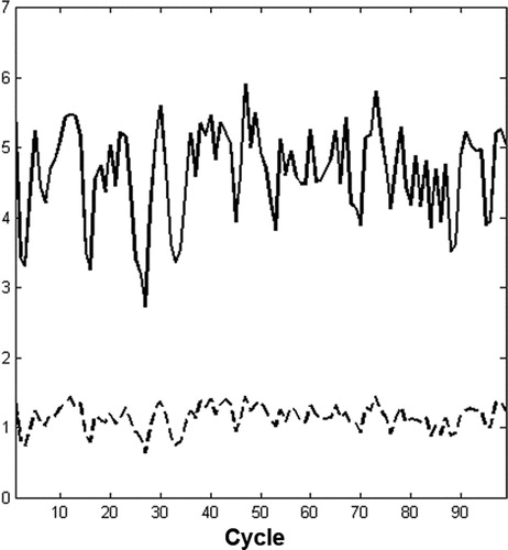
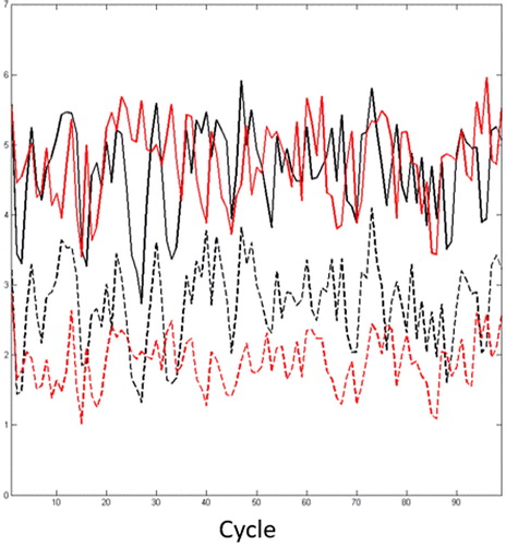
The first two figures below are shown to illustrate the robustness of the assimilation system. Because of the chaotic nature of the model, the representer-based weak constraints 4dvar is carried out with 6 outer loops (Courtier et al. 1994; Bennett et al. 1996) and 125 inner loop iterations, where an inner loop consists of iteratively solving (13). These relatively high numbers of iterations are chosen to allow the minimization to converge, as seen below. The first guess for the representer coefficients vector $\beta$ is set to zero each time (13) is solved. An example of the assimilation’s error reduction is shown in Fig. 1 with the mean absolute error (MAE) in every cycle. Errors in a given solution are defined as the difference from the true solution, i.e. the solution from which the observations are sampled. Two solutions are compared in Fig. 1 through their residuals: the analysis and the background (i.e. the model solution initialized by the assimilation at the end of the previous assimilation cycle). Despite being initialized by the analysis on previous cycles, Fig. 1 shows that the background errors grow quickly in magnitude, due to the analysis residuals from the previous cycle, the chaotic nature of the model, and the rather long assimilation window. As expected the assimilation significantly reduces all the errors in the background.

Fig. 1. MAE of the background (solid line) and analysis (dashed line) errors through all the assimilation cycles.

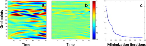
An example of the convergence of the 4dvar minimization process is shown in Fig. 2 for cycle 80 (randomly selected). The representer coefficients after every minimization iteration are used to compute an analysis solution from which the MAE to the true solution is also computed. As the minimization progresses through inner and outer iterations the representer coefficients should converge, leading to the convergence of the analysis. The analysis residuals at the beginning and end of the minimization are shown in Fig. 2, along with the MAE evolution with the minimization iterations. As mentioned above the nonlinear and chaotic nature of the model causes small initial errors from the previous cycle analysis to grow rapidly resulting in a high MAE at the beginning of the minimization. It can be seen in Fig. 2 that errors in some areas of the space-time domain are as high as 15, i.e. 50 observations standard deviations. The errors decrease rapidly in the first two outer loops (from 4.1 to 1.4), and there is only marginal decrease of the analysis errors in the remaining outer loops (from 1.4 to 1.1 in 500 inner iterations). In fact, there is virtually no further decrease in the MAE in the last three outer loops

Fig. 2. Residuals at the beginning (a) and end (b) of the minimization iterations, and MAE of the assimilated solution at every iteration of cycle 80.

4.2. Comparison of pseudo and true ensembles of analyses

We now proceed to the main objective of this study: the approximation of the analysis error covariance by generating an ensemble of pseudo analyses through the perturbation of the optimal representer coefficients. As seen above, the covariance in (24) indicates that the representer coefficients are correlated, and that the perturbations of the representer coefficients should sample the covariance in (24). But the latter is not available. What we do have available is the set of representer coefficients vectors for each minimization iteration. This set of representer coefficients vectors is used to generate a correlation matrix that simulates the correlation in (24). Next, we generate a vector of uncorrelated individual (i.e. component-wise) perturbations from a random normal distribution. This vector has the dimension of the observations space, just as the vector of representer coefficients. We then multiply the correlation matrix with the uncorrelated random vector; this constitutes a perturbation of the representer coefficients vector that we add to the optimal vector to generate one member of the pseudo ensemble of 4dvar analyses. For each perturbed $\beta ,$ a pseudo analysis is computed following (11) and kept as a member of what is referred to as the ensemble of pseudo analyses. According to Fig. 2, convergence of the minimization happens in outer loop 3. Thus, perturbations are generated during the third outer loop, and added to the representer coefficients at the end of the same outer loop 3.

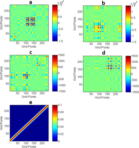
The covariance from this ensemble of pseudo analyses, hereafter referred to as the approximated analysis covariance, is compared to the true analysis error covariance computed from the analytical expression in (16), where the prior error covariance was computed using Monte–Carlo simulations as in Bennett (2002), and all the representer functions for cycles 70 and 80 were also computed. We carried out 1000 Monte–Carlo simulations for the generation of the prior error covariance, and 300 pseudo analyses. Figure 3 shows a comparison of both covariances at the end of the assimilation window for both cycles 70 and 80, and also includes the original prescribed covariance. It can be seen that in general the approximated analysis covariance has lower variance and different correlation patterns than the analytical analysis covariance. The differences between the two covariances are primarily attributed to (1) the neglected perturbation of the background (e.g. Burgers et al., 1998) as mentioned in the approximation (18) and (2) the unknown and unattainable covariance of the optimal representer coefficients (24) from which to draw the perturbations of the representer coefficients. Differences between the two covariances are to be expected, for many reasons: (1) the analytical covariances requires the computation of the error covariance for the model trajectory through Monte–Carlo simulations as well as the computation of all the representer functions. The approximated covariance relies on perturbations of the representer coefficients, with perturbations that are supposed to sample a distribution that is not available. The only source of information about the representer coefficients in a given assimilation cycle is the set of representer coefficients that have already been computed during the minimization. One should keep in mind that the analytical covariance computed here is also an approximation, even though a bigger sample is used for its generation.

Fig. 3. A comparison of the analytical and estimated covariances for cycle 70 (a, b) and cycle 80 (c, d) and the prescribed covariance (e). The analytical covariance used 1000 samples for the prior, and the estimated covariance used 300 members.

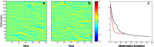
We argue that, although, being different from the analytical analysis covariance, the approximated covariance has more dynamical structure and information than the static Gaussian covariance that was originally prescribed. In fact the approximated analysis covariance at the end of the assimilation window can be used as initial error covariance in the following assimilation window instead of the static covariance. The original assimilation experiment that uses the prescribed static covariances is referred to as experiment 1 (EXP1). An additional experiment, hereafter referred to as experiment 2 (EXP2), is carried out in which the approximated analysis covariance at the end of the assimilation window is used as the initial error covariance for the data assimilation in the following window and so on for all the cycles except the first. No other changes are made in the assimilation process in terms of the minimization method except for the number of inner loops. It was noticed that the minimization process converged faster when using the estimated covariance than the prescribed. EXP2 was set to use only 50 inner loops instead of 125 in EXP1. Thus, in EXP2, only 50 inner loops are used to generate the correlation matrix for perturbing the representer coefficients, still in the third outer loop. Results from EXP2 are compared in Fig. 4 to results from EXP1 in terms of residuals and convergence, for cycle 70 (also randomly selected). The main observation in Fig. 4 is that the analysis residuals from both experiments are similar. Residuals from EXP1 are marginally lower that their EXP2 counterpart. This is due to the fact that EXP2 uses significantly less iterations. EXP2 was set to run with 6 outer loops of 50 inner iterations each. The evolution of the MAE with minimization iterations shows that EXP2 has the same level of errors after 300 minimization iterations as EXP1. Thus, the marginally lower residuals from EXP1 are only due to its additional 450 minimization iterations. Figure 4 also shows that EXP2 converges in about 100 to 150 iterations.

Fig. 4. A comparison of cycle 70 residuals at the end of the minimization with the prescribed covariance (a), the estimated covariance (b) and the evolution of the residual norm (c) using the prescribed covariance (black) and the estimated covariance (red).

This is an encouraging unintended development, since convergence was not an objective of the study, and exploring the reasons for the faster convergence of EXP2 is beyond the scope of the study. Nonetheless, we examine whether the rapid convergence of EXP2 is consistent throughout the cycles by computing the MAE of the background and analysis after 100 iterations for both EXP1 and EXP2. It can be seen in Fig. 5 that, although, the two background solutions have similar error levels, EXP2 has consistently lower errors after 100 iterations than EXP1. The estimated covariance thus seems to be more effective than the static prescribed covariance. It can be seen from Fig. 3 that the estimated covariance is arguably a better approximation to the analytical covariance than the prescribed static covariance.

Fig. 5. Mean absolute error of the background (solid lines) and analysis (dashed lines) from EXP1 (black) and EXP2 (red). The analyses are computed after 100 minimization iterations.

5. Discussion

The method proposed here alleviates the burden of carrying out an EDA experiments (only one minimization is performed), and provides an estimate of the analysis covariance, not just the variances. This method is clearly different from the hybrid methods. It may appear that the prescribed static covariance was inadequate for the data assimilation problem posed in this study. It is possible to tune the parameters of the prescribed covariance in order to improve the results of the assimilation for a given set of observations. This is a tedious and time consuming process that has to be repeated every assimilation cycle, and as such should be avoided. The study at hand is not about the proper prescription of prior covariances, but the estimation of the posterior covariances once the prior have been prescribed. The proposed method simplifies such a process (there is no need to guess the correlation scales or variances) and improves the analysis results. The posterior covariance is still needed and computationally costly to obtain even for adequately prescribed prior covariances and a well-conditioned minimization for the data assimilation problem. The method described here, although, lacking perturbations of the background solution, still yields a flow-dependent covariance that is a better approximation to the analytic than the prescribed. This is probably the reason for better results from EXP2. This study shows that the time-consuming and computationally costly process of guessing the covariances can be avoided by adopting the posterior covariances at the end of the assimilation window for initial error covariance for the following assimilation window.

In the case of the classic strong constraints 4dvar, one can still apply the method proposed here by perturbing the optimal adjoint at the initial time. However, it may still be preferable to use perturbations of the optimal representer coefficients for two reasons. First, the observations space is usually smaller than the initial conditions space, and second, the validity of the tangent linear approximation that enables the strong constraints also ensures that the representer method with no model error yields the same solution as the strong constraints 4dvar. However, with the classic strong constraints 4dvar the ensemble of pseudo analyses will consist of solutions of the nonlinear model instead of the linearized model used in the representer method. Still, both methods will yield a flow dependent covariance in which cross correlations are determined by the dynamics of the nonlinear (strong constraints) or linearized (representer) model. The application of the method proposed here to realistic models of the atmosphere or ocean for which a 4dvar system exists, and comparisons with an ensemble of 4dvar analyses, should be straightforward.

5.1 The computational cost

Given sufficient resources, parallel computing provides the ability to generate an ensemble of model solutions simultaneously, i.e. for the same wall-clock time it take to obtain one model solution. This is the reason why ensemble-based data assimilation is said to be ‘embarrassingly parallel’. Assuming that N computer nodes are needed for one model solution, the same N nodes are used for the 4dvar system, in the sequential application of the forward and adjoint models, or adjoint and tangent linear models. The wall-clock time of the 4dvar system is thus driven by the iterative minimization process. An ensemble of 4dvar solutions of size M requires MN computer nodes with no additional wall-clock time. The method proposed in this study requires only the N nodes for one 4dvar analysis. The additional applications of the final sweep to generate the ensemble of pseudo analyses also requires MN nodes, all in parallel with the final sweep of the underlying 4DVAR. Therefore, the generation of the ensemble of pseudo analyses does not require additional wall-clock. In general, a large ensemble size (M > 100) is needed to avoid sampling errors in the covariance. It is doubtful that 100 N nodes are available during each assimilation cycle, and for the time it takes for 4dvar analysis, when N itself is already large.

We denote by F_C the cost of a final sweep (in the representer method) in CPU time. It comprises the cost of the adjoint model, the covariance multiplication, and the tangent linear model. If K minimization iterations are needed, the 4dvar is (K + 1)F_C. The cost of an M-sized ensemble of 4dvar analyses is M(K + 1)F_C, while a similarly sized ensemble of pseudo analyses by the proposed method costs (K + M)F_C. Note that the 4dvar solution is counted as a member of the ensemble of pseudo analyses. The difference in CPU time is K(M – 1) F_C, which increases with both M and K. Thus, the ensemble of 4dvar analyses will always require more resources than the method proposed in this study.

6. Summary

A method for estimating the analysis error covariance in a 4dvar data assimilation is proposed. It consists of perturbing the optimal representer coefficients and generating an ensemble of pseudo analyses (E_PA), one per each perturbed vector of representer coefficients, through the final sweep of the representer method. The method was applied to the Lorenz-2005 model, in a twin-data assimilation experiment. The estimated covariance at the end of the assimilation window was compared to its theoretical counterpart. It was found that the estimated covariance had slightly lower variances and weaker correlations. In addition, an experiment in which the estimated covariance at the end of the assimilation cycle was used as initial error covariance in the following cycle produced analyses with similar error levels as the original experiment, but consistently converged faster throughout the cycles.

By perturbing only the representer coefficients, which are defined in the observations space, the method proposed here neglects the potential contribution of the perturbations of the background solution (as a truly perturbed analysis would require) to the perturbations of the representer functions elsewhere in the model domain. The proposed method applies the Monte–Carlo technique to the final sweep of the representer method, a significantly less expensive way of generating an ensemble of pseudo analyses. A large ensemble size is, therefore, achievable with no additional wall-clock time, since only one assimilation minimization is required, and each member of the ensemble can be generated in parallel with the 4dvar final sweep.

Acknowledgement

The authors would like to thank the anonymous reviewers for their comments that contributed to improve the quality of the manuscript.

Disclosure statement

No potential conflict of interest was reported by the authors.

Additional information

Funding

This work was sponsored by the Office of Naval Research Program Element 62435N as part of the ‘‘Coupled Ocean-Atmosphere variational assimilation and prediction system’’ project. This paper is NRL paper contribution number NRL/JA/7320-19-4647.

Appendix

For the sake of clarity and for readers who are not familiar with the representer method (Bennett 2002) this appendix details how the adjoint solution is computed given the representer coefficients. The inner loop of the assimilation system attempts to solve (4(4) $$\{\begin{array}{l}\frac{\partial \widehat{u}}{\partial t}=L\left(\widehat{u}\right)+F+C_f•\lambda ,\\ \widehat{u}\left(x,0\right)=I\left(x\right)+ C_i\circ \lambda (x,0),\\ -\frac{\partial \lambda }{\partial t}={\left[\frac{\partial L}{\partial u}\left(\widehat{u}\right)\right]}^T\lambda +\sum _{m=1}^M\sum _{n=1}^M{W}_{\epsilon ,mn}\left(y_m-H_m\widehat{u}\right)H_n^T\delta \left(x-x_n\right)\delta \left(t-t_n\right),\\ \lambda (x,T)=0,\end{array}$$(4) ) using the expansion (11(11) $$\widehat{u}(x,t)=u_F(x,t)+\sum _{m=1}^M{\beta }_m{r}_m(x,t),$$(11) ) in which the representer functions and adjoint representer functions are defined in (12(12) $$\{\begin{array}{l}\frac{\partial r_m}{\partial t}=\mathrm{L}{r}_m+C_f•{\alpha }_m(x,t),\\ r_m\left(x,0\right)= C_i\circ {\alpha }_m(x,0),\\ -\frac{\partial {\alpha }_m}{\partial t}={\mathrm{L}}^T{\alpha }_m+H_m^T\delta \left(x-x_m\right)\delta \left(t-t_m\right),\\ {\alpha }_m(x,T)=0,\end{array}$$(12) ). We use the following notations for the differential operators (A1) $$D=\frac{\partial }{\partial t}-\mathrm{L}$$(A1) and (A2) $$D^T=-\frac{\partial }{\partial t}-{\mathrm{L}}^T$$(A2)

Applying the differential operator (A1(A1) $$D=\frac{\partial }{\partial t}-\mathrm{L}$$(A1) ) to the linear expansion (11(11) $$\widehat{u}(x,t)=u_F(x,t)+\sum _{m=1}^M{\beta }_m{r}_m(x,t),$$(11) ) gives (A3) $$D\widehat{u}=D{u}_F+\sum _{m=1}^M{\beta }_{m}D{r}_m=F+\sum _{m=1}^M{\beta }_m{C}_f•{\alpha }_m.$$(A3)

By virtue of (A3(A3) $$D\widehat{u}=D{u}_F+\sum _{m=1}^M{\beta }_{m}D{r}_m=F+\sum _{m=1}^M{\beta }_m{C}_f•{\alpha }_m.$$(A3) ) and the definitions (5(5) $$\lambda (x,t)=\underset{0}{\overset{T}{\int }}\underset{\Omega }{\overset{}{\int }}{W}_f\left(x,t,x\prime ,t\prime \right)f\left(x\prime ,t\prime \right)dx\prime dt\prime ,$$(5) ) and (6(6) $$C_f•\lambda (x,t)=\underset{0}{\overset{T}{\int }}\underset{\Omega }{\overset{}{\int }}{C}_f\left(x,t,x\prime ,t\prime \right)\lambda \left(x\prime ,t\prime \right)dx\prime dt\prime ,$$(6) ) we get (A4) $$\lambda =C_f^{-1}•f=C_f^{-1}•\left[D\widehat{u}-\mathrm{ }F\right]=\sum _{m=1}^M{\beta }_m{\alpha }_m(x,t)$$(A4)

Also, applying the differential operator (A2) to (A4) results in (A5) $$D^T\lambda =\sum _{m=1}^M{\beta }_m{D}^T{\alpha }_m=\sum _{m=1}^M{\beta }_m{H}_m^T\delta \left(x-x_m\right)\delta \left(t-t_m\right),$$(A5) from the definition of the adjoint representer functions in (12(12) $$\{\begin{array}{l}\frac{\partial r_m}{\partial t}=\mathrm{L}{r}_m+C_f•{\alpha }_m(x,t),\\ r_m\left(x,0\right)= C_i\circ {\alpha }_m(x,0),\\ -\frac{\partial {\alpha }_m}{\partial t}={\mathrm{L}}^T{\alpha }_m+H_m^T\delta \left(x-x_m\right)\delta \left(t-t_m\right),\\ {\alpha }_m(x,T)=0,\end{array}$$(12) ), and from the Euler–Lagrange system (4(4) $$\{\begin{array}{l}\frac{\partial \widehat{u}}{\partial t}=L\left(\widehat{u}\right)+F+C_f•\lambda ,\\ \widehat{u}\left(x,0\right)=I\left(x\right)+ C_i\circ \lambda (x,0),\\ -\frac{\partial \lambda }{\partial t}={\left[\frac{\partial L}{\partial u}\left(\widehat{u}\right)\right]}^T\lambda +\sum _{m=1}^M\sum _{n=1}^M{W}_{\epsilon ,mn}\left(y_m-H_m\widehat{u}\right)H_n^T\delta \left(x-x_n\right)\delta \left(t-t_n\right),\\ \lambda (x,T)=0,\end{array}$$(4) ), then, we get (A6) $$D^T\lambda =\sum _{m=1}^M\sum _{n=1}^M{W}_{\epsilon ,mn}\left(y_m-H_m\widehat{u}\right)H_n^T\delta \left(x-x_n\right)\delta \left(t-t_n\right).$$(A6)

Once the representer coefficients are computed (below) Equation (A5)(A5) $$D^T\lambda =\sum _{m=1}^M{\beta }_m{D}^T{\alpha }_m=\sum _{m=1}^M{\beta }_m{H}_m^T\delta \left(x-x_m\right)\delta \left(t-t_m\right),$$(A5) shows how the adjoint solution is obtained. Note that, although, the representer coefficients are defined in the observations space, the adjoint solution is defined over the entire space-time data assimilation domain.

Equating the right-hand sides of (A5(A5) $$D^T\lambda =\sum _{m=1}^M{\beta }_m{D}^T{\alpha }_m=\sum _{m=1}^M{\beta }_m{H}_m^T\delta \left(x-x_m\right)\delta \left(t-t_m\right),$$(A5) ) and (A6(A6) $$D^T\lambda =\sum _{m=1}^M\sum _{n=1}^M{W}_{\epsilon ,mn}\left(y_m-H_m\widehat{u}\right)H_n^T\delta \left(x-x_n\right)\delta \left(t-t_n\right).$$(A6) ) gives (A7) $${\beta }_m=\sum _{n=1}^M{W}_{\epsilon ,mn}\left(y_n-H_n\widehat{u}\right).$$(A7)

In (A7(A7) $${\beta }_m=\sum _{n=1}^M{W}_{\epsilon ,mn}\left(y_n-H_n\widehat{u}\right).$$(A7) ) the representer coefficients still depend on the unknown optimal solution $\widehat{u}.$ Substituting the linear expansion (11(11) $$\widehat{u}(x,t)=u_F(x,t)+\sum _{m=1}^M{\beta }_m{r}_m(x,t),$$(11) ) into (A7(A7) $${\beta }_m=\sum _{n=1}^M{W}_{\epsilon ,mn}\left(y_n-H_n\widehat{u}\right).$$(A7) ) with some rearranging leads to the linear system (13(13) $$\left({\mathrm{R}+\mathrm{C}}_{\mathrm{\epsilon }}\right)\widehat{\beta }={\mathrm{y}-\text{Hu}}_{\mathrm{F}},$$(13) ). Thus, using the representer method for solving the Euler–Lagrange system (4(4) $$\{\begin{array}{l}\frac{\partial \widehat{u}}{\partial t}=L\left(\widehat{u}\right)+F+C_f•\lambda ,\\ \widehat{u}\left(x,0\right)=I\left(x\right)+ C_i\circ \lambda (x,0),\\ -\frac{\partial \lambda }{\partial t}={\left[\frac{\partial L}{\partial u}\left(\widehat{u}\right)\right]}^T\lambda +\sum _{m=1}^M\sum _{n=1}^M{W}_{\epsilon ,mn}\left(y_m-H_m\widehat{u}\right)H_n^T\delta \left(x-x_n\right)\delta \left(t-t_n\right),\\ \lambda (x,T)=0,\end{array}$$(4) ) involves two steps: solving the linear system (13(13) $$\left({\mathrm{R}+\mathrm{C}}_{\mathrm{\epsilon }}\right)\widehat{\beta }={\mathrm{y}-\text{Hu}}_{\mathrm{F}},$$(13) ) to obtain the representer coefficients, and then substituting the latter into (A5) to obtain the optimal adjoint solution that will in turn be substituted into the first two equations of the Euler–Lagrange system (4(4) $$\{\begin{array}{l}\frac{\partial \widehat{u}}{\partial t}=L\left(\widehat{u}\right)+F+C_f•\lambda ,\\ \widehat{u}\left(x,0\right)=I\left(x\right)+ C_i\circ \lambda (x,0),\\ -\frac{\partial \lambda }{\partial t}={\left[\frac{\partial L}{\partial u}\left(\widehat{u}\right)\right]}^T\lambda +\sum _{m=1}^M\sum _{n=1}^M{W}_{\epsilon ,mn}\left(y_m-H_m\widehat{u}\right)H_n^T\delta \left(x-x_n\right)\delta \left(t-t_n\right),\\ \lambda (x,T)=0,\end{array}$$(4) ) for the optimal model solution. This procedure holds for both strong and weak constraints, the only difference being the absence or presence of the model error covariance in the strong constraints. Note that the traditional strong constraints uses the nonlinear forward model. However, since we are computing an increment/correction to the first guess in either strong or weak constraints, the forward dynamics can be replaced by the tangent linear model as long as it is valid, and the first guess can be computed with the full nonlinear model. ${\lambda }_0$ is a full field.

References

- Amodei, L. 1995. Solution approchée pour un problème d’assimilation de données avec prise en compte de l’erreur du modèle. C. R. Acad. Sci. 321, Série IIa, 1087–1094.
- Auligné, T., Ménétrier, B., Lorenc, A. and Buehner, M. 2016. Ensemble-variational integrated localized data assimilation. Mon. Weather Rev. 144, 3677–3696. doi:10.1175/MWR-D-15-0252.1
- Belo Pereira, M. and Berre, L. 2006. The use of an ensemble approach to study the background error covariances in a global NWP model. Mon. Weather Rev. 134, 2466–2498. doi:10.1175/MWR3189.1
- Bennett, A. F. 1992. Inverse Methods in Physical Oceanography. Cambridge University Press, New York, pp. 347.
- Bennett, A. F. 2002. Inverse Modeling of the Ocean and Atmosphere. Cambridge University Press, New York, pp. 234.
- Bennett, A. F., Chua, B. S. and Leslie, L. M. 1996. Generalized inversion of a global numerical weather prediction model. Meteorl. Atmos. Phys. 60, 165–178. doi:10.1007/BF01029793
- Bonavita, M., Isaksen, L. and Hólm, E. 2012. On the use of EDA background error variances in the ECMWF 4D-Var. Q. J. R. Meteorol. Soc. 138, 1540–1559. doi:10.1002/qj.1899
- Bousserez, N., Henze, D. K., Perkins, A., Bowman, K. W., Lee, M. and co-authors. 2015. Improved analysis-error covariance matrix for high-dimensional variational inversions: application to source estimation using a 3D atmospheric transport model. Q. J. R. Meteorol. Soc. 141, 1906–1921. doi:10.1002/qj.2495
- Burgers, G., Jan van Leeuwen, P. and Evensen, G. 1998. Analysis scheme in the ensemble Kalman filter. Mon. Weather Rev. 126, 1719–1724. doi:10.1175/1520-0493(1998)126<1719:ASITEK>2.0.CO;2
- Cheng, H., Jardak, M., Alexe, M. and Sandu, A. 2010. A hybrid approach to estimating error covariances in variational data assimilation. Tellusa. 62, 288–297. doi:10.1111/j.1600-0870.2009.00442.x. doi:10.1111/j.1600-0870.2010.00442.x
- Courtier, P., Thépaut, J.-N. and Hollingsworth, A. 1994. A strategy for operational implementation of 4D-Var, using an incremental approach. Q. J. R. Meteorol. Soc. 120, 1367–1387. doi:10.1002/qj.49712051912
- Daget, N., Weaver, A. and Balmaseda, M. 2009. Ensemble estimation of background-error variances in a three-dimensional variational data assimilation system for the global ocean. Q. J. R. Meteorol. Soc. 135, 1071–1094. doi:10.1002/qj.412
- Egbert, G. D., Bennett, A. F. and Foreman, M. G. G. 1994. TOPEX/POSEIDON tides estimated using a global inverse method. J. Geophys. Res. 99, 24821–24852. doi:10.1029/94JC01894
- Fairbairn, D., Pring, S. R., Lorenc, A. C. and Roulstone, I. 2014. A comparison of 4DVar with ensemble data assimilation methods. Q. J. R. Meteorol. Soc. 140, 281–294. doi:10.1002/qj.2135
- Gejadze, I. Y., Shutyaev, V., L. and Dimet, F.-X. 2013. Analysis error covariance versus posterior covariance in variational data assimilation. Q. J. R. Meteorol. Soc. 139, 1826–1841. doi:10.1002/qj.2070
- Kalnay, E. 2003. Atmospheric Modeling, Data Assimilation and Predictability. Cambridge University Press, Cambidge, pp. 341.
- Lorenz, E. N. 2005. Designing chaotic models. J. Atmos. Sci. 62, 1574–1587. doi:10.1175/JAS3430.1
- Moore, A. M., Arango, H. and Broquet, G. 2012. Estimates of analysis and forecast error variances derived from the adjoint of 4D-Var. Mon. Weather Rev. 140, 3183–3203. doi:10.1175/MWR-D-11-00141.1
- Ngodock, H. E. and Carrier, M. J. 2014. A 4DVAR system for the navy coastal ocean model. Part 1: system description and assimilation of synthetic observations in Monterey Bay. Mon. Weather Rev. 142, 2085–2107. doi:10.1175/MWR-D-13-00221.1
- Shutyaev, V., Gejadze, I., Copeland, G. J. M. and Le Dimet, F.-X. 2012. Optimal solution error covariance in highly nonlinear problems of variational data assimilation. Nonlin. Processes Geophys. 19, 177–184. doi:10.5194/npg-19-177-2012
- Zagar, N., Andersson, E. and Fisher, M. 2005. Balanced tropical data assimilation based on a study of equatorial waves in ECMWF short-range forecast errors. Q. J. R. Meteorol. Soc. 131, 987–1011. doi:10.1256/qj.04.54