Occurrence and drivers of wintertime temperature extremes in Northern Europe during 1979–2016

Abstract

Applying the daily ERA-interim reanalysis data from 1979 to 2016, we found that widespread cold (warm) wintertime extreme events in Northern Europe occurred most frequently in winter 1984–1985 (2006–2007). These events often persisted for multiple days, and their primary drivers were the pattern of atmospheric large-scale circulation, the direction of surface wind and the downward longwave radiation. Widespread cold extremes were favoured by the Scandinavian Pattern and Ural Blocking, associated with advection of continental air-masses from the east, clear skies and negative anomalies in downward longwave radiation. In the case of widespread warm extremes, a centre of low pressure was typically located over the Barents Sea and a centre of high pressure over Central Europe, which caused south-westerly winds to dominate over Northern Europe, bringing warm, cloudy air masses to Northern Europe. Applying Self-Organizing Maps, we found out that thermodynamic processes explained 80% (64%) of the decreasing (increasing) trend in the occurrence of extreme cold (warm) events. The trends were due to a combined effect of climate warming and internal variability of the system. Changes in cases with a high-pressure centre over Iceland were important for the decreased occurrence of cold extremes over Northern Europe, with contribution from increasing downward long-wave radiation and south-westerly winds. The largest contribution to the increased occurrence of widespread warm extremes originated from warming and increased occurrence of the Icelandic low.

Keywords:

• Northern Europe
• extreme temperature events
• Scandinavian Pattern
• Icelandic low
• Self-Organizing Maps (SOM)

1. Introduction

There is increasing scientific and public attention to extreme events in the changing climate system (Wang et al., 2017). A large inter-annual and decadal variability of the climate system is superimposed to the global warming trend, and the variability is particularly prominent in the mid- and high-latitudes (Shepherd, 2014, 2015; McKinnon and Deser, 2018). The warming trend as well as its inter-annual and decadal variations also affect the occurrence of regional weather extremes (Screen and Simmonds, 2014). The changes in climate variables, such as air temperature, and the frequency of occurrence of extremes of these variables, can in principle be separated in forced responses to drivers of the climate system and the underlying chaotic natural variability of the system (Barnes et al., 2019). From another point of view, the separation can be made with respect to changes driven by thermodynamic and dynamic processes (Sillmann et al., 2017). The separation is in any case challenging, and further complicated by the fact that a forced dynamic or thermodynamic response may appear in the same form as some of the modes of the internal variability of the climate system (Shepherd, 2014). To meet this challenge, ensembles of climate model simulations (Deser et al., 2017; McKinnon and Deser, 2018; Barnes et al., 2019), sophisticated statistical methods (Horton et al., 2015) and artificial intelligence (Barnes et al., 2019) have been applied.

Several studies have addressed changes in the occurrence and magnitude of air temperature extremes in Northern Europe (Tuomenvirta et al., 2000; Beniston et al., 2007; Räisänen and Ruokolainen, 2008; Jaagus et al., 2014; Kivinen et al., 2017; Vihma et al., 2020). In Northern Europe, the climate warming is faster than the global mean (Rutgersson et al., 2015), but also the inter-annual and decadal variations are large in Northern Europe (Yang et al., 2012; Räisänen, 2019), which makes it difficult to robustly attribute the observed changes in extreme temperatures. Observations from the northernmost Fenno-Scandia show a very high frequency of warm weather events in the period 2000–2014 and in the future, with continued global warming, their occurrence is expected to further increase (Vikhamar-Schuler et al., 2016). More frequently occurring extreme temperatures are likely to have major impacts on hydrological, geophysical, ecological and socio-economic systems in Northern Europe.

Considering drivers of winter weather in Northern Europe, the most well-known is the North Atlantic Oscillation (NAO). Its negative phase is associated with cold winters and positive phase with warm winters in Northern Europe (Marshall et al., 2001; Hurrell and Deser, 2009; Deser et al., 2017). Other well know drivers include the Scandinavian Pattern (SCA; Vihma et al., 2020), the Greenland Blocking (Hanna et al., 2018), the East Atlantic Pattern (Comas-Bru and McDermott, 2014) and the East Atlantic/West Russia Pattern (Lim, 2015). Conditions in the central Arctic and the Greenland, Norwegian, Barents and Kara seas also affect Northern Europe controlling the upstream conditions for cold-air outbreaks and polar lows, which often reach Northern Europe (Walsh et al., 2001). Due to the amplified climate warming in the Arctic, wintertime warm extremes have become increasingly common and stronger in the Central Arctic, the positive anomalies reaching up to 30 °C in individual days (Matthes et al., 2015; Graham et al., 2017). In contrast, mid-latitude regions have frequently experienced very cold or snow-rich events over the latest decades (Vihma, 2017; Vavrus, 2018; Cohen et al., 2020). However, the linkages between the Arctic warming and European weather and climate have been less clear than those between the Arctic and East-Asia or North America (Overland et al., 2015). According to some studies, the Arctic warming favours the negative phase of NAO (Kim et al., 2014; Nakamura et al., 2015; Deser et al., 2016), which would yield a dynamic effect of cold winter anomalies over Europe, tending to compensate for the greenhouse warming. However, not all studies have supported the negative NAO response to Arctic warming (Screen et al., 2014; Smith et al., 2017).

Understanding the drivers of extreme weather events that have occurred in the past is pivotal for predicting future evolution of occurrence of weather extremes in Northern Europe. The need for further research is also motivated by the importance of wintertime temperature and precipitation extremes on ecosystems (Wrona et al., 2016) and societies, at least in the fields of winter tourism (Steiger et al., 2019), reindeer herding (Vors and Boyce, 2009) and hydropower production (Instanes et al., 2016; Shevnina et al., 2019). In this article, we study the wintertime temperature extremes in Northern Europe during 1979–2016. In Section 2, we introduce the data and methods used. In Section 3, we present the results and evaluate the reasons for extreme events in Northern Europe, followed by discussion in Section 4.

2. Data and methods

The data we used is from the global daily ERA-Interim reanalysis, produced by the European Centre for Medium-Range Weather Forecasts (Dee et al., 2011). The product has a horizontal resolution of 0.75° × 0.75° in a latitude-longitude coordination. We focused on winter and defined winter 1979 as December 1979, January 1980 and February 1980, and analogously for the following years. We defined temperature extremes using the 2-m air temperature data. Besides, we used data on sea-level pressure (SLP), wind speed and direction, downward long-wave radiation, as well as vertically-integrated cloud frozen water and cloud liquid water.

Warm/cold extreme thresholds were defined as the 99th/1st percentile value of the daily 2-m air temperature anomaly. The anomalies were calculated for each grid cell with respect to the mean over the climatological normal period 1981–2010. We defined a widespread extreme day so that at least 50 grid points in the study region should exceed the warm threshold or be below the cold threshold. Further, the sensitivity of the results to the thresholds with respect to the percentile value and the number of grid points was tested. The number of events meeting the criteria of temperature extremes naturally depended on the thresholds, but the main results, such as the trends in the occurrence of warm and cold extremes, were not sensitive to the thresholds. We applied composite analysis to explore the relationship between the large-scale circulation variability and extreme temperature events. In addition, regression analysis was used to detect the atmospheric circulation patterns most commonly associated with various extreme temperature patterns. We used Mann-Kendall non-parametric test for monotonic trend, and trends surpassing the 5% significance threshold were considered statistically significant.

Further, we applied the Self-Organizing Maps (SOM) method. It is based on a neural network algorithm that groups similar data records together, and then reduces the dimensions of large data sets by organizing them into a two-dimensional array (Kohonen, 2001). The SOM method uses unsupervised learning to determine generalised patterns in data. It captures the distribution of the data so that the algorithm tends to minimise the average differences between the samples in the dataset (Johnson et al., 2008). Although its use in meteorological applications is increasing (e.g. Nygård et al., 2019), SOM is still a relatively new method to study extreme weather events. The circulation patterns achieved from SOM can help to understand linkages between large-scale atmospheric circulation and local meteorological variables (Gibson et al., 2016; Yu et al., 2018). Focusing on temperature, Loikith and Broccoli (2015) used SOM to evaluate differences between climate models and observations in temperature extremes related to circulation patterns. Horton et al. (2015) used the SOM method to study trends of temperature extremes, and suggested that changes in extreme temperature trends were related to the frequency of geopotential height patterns. The SOM method was also used to evaluate temperature and wind extremes (Cassano et al., 2006) and other temperature anomalies (Cassano et al., 2011) in Alaska. Later, Cassano et al. (2016) focused on how to choose an optimal SOM for analysing extreme events, paying attention to the advantages and disadvantages of using various numbers of patterns.

As many of the above-mentioned papers have presented details of the SOM algorithm, we only present the approach of this study in classifying the wintertime large-scale circulation using daily SLP anomalies for DJF from 1979 to 2016. The SLP anomalies were calculated for each day for each grid cell as a difference between each day’s mean SLP and the mean SLP over the period 1981–2010. After considering experiences from many previous SOM-based meteorological studies, we chose to use a SOM matrix consisting of 12 patterns (often called nodes). Then the individual daily SLP anomaly fields were mapped to the SOM by associating each daily SLP sample with a single pattern on the SOM by root-mean-square error (RMSE), which is used as a metrics to measure how well each SOM node matches the daily SLP field.

Following Cassano et al. (2007), the frequency of extreme temperature occurrence (E) can be presented as the sum of occurrences of extreme temperatures associated with each SOM node: (1) $$E=\sum _{i=1}^K{E}_i{f}_i=\sum _{i=1}^K(\overline{E_i}+{E_i}^{\mathrm{\prime }})(\overline{f_i}+{f_i}^{\mathrm{\prime }})$$(1) where$\mathrm{ }{f}_i$ is the frequency of occurrence of SOM node$\mathrm{ }i,$$\mathrm{ }{E}_i$ is the frequency of extreme temperature occurrence when SOM node $i$ occurs and $K$ is the total number of SOM nodes ($\text{in our case},\mathrm{ }K=12$). The bars and primes denote the time mean and deviation from it, respectively. The temporal change (trend) in E is obtained by differentiating Eq. (1)(1) $$E=\sum _{i=1}^K{E}_i{f}_i=\sum _{i=1}^K(\overline{E_i}+{E_i}^{\mathrm{\prime }})(\overline{f_i}+{f_i}^{\mathrm{\prime }})$$(1) with respect to time: (2) $$\frac{dE}{dt}=\sum _{i=1}^K[\overline{f_i}\frac{d{E_i}^{\mathrm{\prime }}}{dt}+\overline{E_i}\frac{d{f_i}^{\mathrm{\prime }}}{dt}+\frac{d\left({E_i}^{\mathrm{\prime }}{f_i}^{\mathrm{\prime }}\right)}{dt}]$$(2)

The right-hand side of Eq. (2)(2) $$\frac{dE}{dt}=\sum _{i=1}^K[\overline{f_i}\frac{d{E_i}^{\mathrm{\prime }}}{dt}+\overline{E_i}\frac{d{f_i}^{\mathrm{\prime }}}{dt}+\frac{d\left({E_i}^{\mathrm{\prime }}{f_i}^{\mathrm{\prime }}\right)}{dt}]$$(2) shows, from left to right, the thermodynamic, dynamic and interaction contributions for the total trend associated with each SOM node$\mathrm{ }i.$ Following Horton et al. (2015), for the thermodynamic contribution, we assume that each SOM pattern is stationary over the study period, and that trends in the occurrence of extreme temperatures result from factors unrelated to atmospheric circulation, such as increase in downward long-wave radiation due to increasing greenhouse gas concentrations, or changes in the air-surface exchange of heat and moisture. The thermodynamic contribution associated with each SLP anomaly pattern is determined by the product of the mean occurrence of the SOM pattern ($\overline{f_i}$) and the trend in extreme temperature occurrence per SOM pattern occurrence ($\frac{d{E_i}^{\mathrm{\prime }}}{dt}$).The dynamic contribution assumes that each SOM pattern is stationary, and the frequency of occurrence of extreme events results from the changes in the occurrence of each SOM pattern. The dynamic contribution is determined by the product of the trend in the occurrence of each SOM pattern ($\frac{d{f_i}^{\mathrm{\prime }}}{dt}$) and the mean number of extreme events per SOM pattern occurrence ($\overline{E_i}$). The third component results from the trend of $E_i^{\mathrm{\prime }}{f}_i^{\mathrm{\prime }},\mathrm{ }$ i.e. the product of the anomaly in extreme temperature occurrence per SOM pattern occurrence and anomaly in the SOM pattern occurrence. The product $E_i^{\mathrm{\prime }}{f}_i^{\mathrm{\prime }}$ can be negative, zero or positive. The interaction component is positive, for example, if in the beginning of the study period the anomalies (calculated, e.g. for a season or a year) $E_i^{\mathrm{\prime }}\text{ and }{f}_i^{\mathrm{\prime }}\mathrm{ }$ have the opposite sign but have the same sign towards the end of the time series. Analogously, a change towards the opposite sign of $E_i^{\mathrm{\prime }}\text{ and }{f}_i^{\mathrm{\prime }}$ results in a negative interaction component. The trend in the product $E_i^{\mathrm{\prime }}{f}_i^{\mathrm{\prime }}$ cannot be physically interpreted solely as a dynamic or thermodynamic contribution to the trend in the occurrence of extreme temperatures. Although it is called the interaction component, it does not necessarily represent any particular physical interaction process, but mathematically represents the contribution of the trend of $E_i^{\mathrm{\prime }}{f}_i^{\mathrm{\prime }}$ to the trend in$\mathrm{ }E.$ Various meteorological processes and events may result in or be randomly associated with similar or opposite signs of $E_i^{\mathrm{\prime }}\text{ and }{f}_i^{\mathrm{\prime }}.$ In Section 3, we present examples of SOM nodes having a strong interaction component.

3. Results

3.1. Occurrence of extreme temperatures

Figure 1 shows the study area (5–40^oE, 55–70^oN) and surrounding region. According to definition of widespread temperature extremes, we compute the cold and warm days in Northern Europe, and present the statistical results in Fig. 2 and Table 1. Figure 2 shows the total number of widespread cold and warm extreme days for each grid cell of the ERA-Interim reanalysis during 1979–2016, and the number of widespread cold and warm extreme days per winter from 1979 to 2016. As the number of local extremes is the same (1% of the data) in each grid cell, the maxima in the spatial distributions indicate grid cells which often belong to the regions covered by widespread extreme events. In general, such grid cells dominate in the eastern and southern parts of the study region (Fig. 2a,b).

Fig. 1. The studying area. The blue box indicates the region where widespread extreme events were identified.

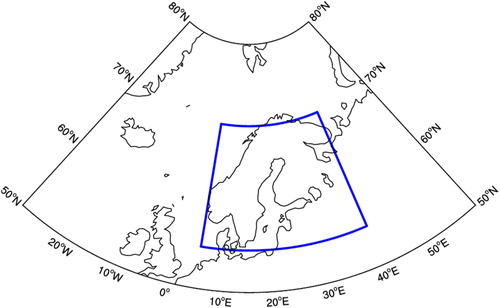
Fig. 2. The total number of days of widespread (a) extremely cold and (b) extremely warm temperatures for each grid cell of the ERA-Interim reanalysis during 1979–2016, (c) the number of widespread extremely cold (blue bars) and warm (red bars) days per winter from 1979 to 2016 and (d) PDF of air temperature anomaly in the study area for 2006–2016 (red line) and 1979–1989 (blue line). The anomalies are calculated with respect to the reference period of 1981–2010. The dashed lines stand for quantiles of 95% and 99%.

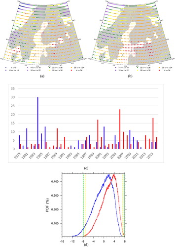
Table 1. The number of extreme days, single-day events, all multiday events and events lasting for four or more days.

Extreme type	Extreme days	Single-day events	Multiday events	Long events
DJF cold	165	26 (15.8%)	34 (84.3%)	16 (58.2%)
DJF warm	179	43 (24.0%)	42 (76.0%)	8 (35.2%)

Considering the time series (Fig. 2c), the number of widespread cold extreme days was largest (30) in 1984, while the number of widespread warm extreme days was largest (23) in 2006. The majority of the cold extreme days occurred during 1979–1986, and far less cold extremes occurred between 1987 and 1994, but after 1994 the numbers were again higher, especially in 2002 and 2009. The majority of warm extremes occurred after 2000, with 2006, 2015 and 2000 as the top three winters. Prior to 2000, the number of extremely warm days per winter did not exceed 7 days, except in the winter of 1989. The declines in extremely cold days (no statistically significant trend) and significant increases in extremely warm days are consistent with Kivinen et al. (2017). We further computed the probability density function (PDF) of the daily temperature anomaly using the reference period of 1981–2010. To illustrate the decadal change, we compared the PDFs of the first 10 years 1979–1989 and the last 10 years 2006–2016 in Fig. 2d. According to Kodra and Ganguly (2014) the tail of the PDF can be influenced by a shift in the mean value, an increased variability and a changed symmetry for a certain distribution. On the basis of our result, we suggest that the shift in the mean value is the main reason for the change in the PDF of air temperature anomaly in Northern Europe, resulting in an increase in the occurrence of the extremely warm events and a decrease in the occurrence of extremely cold events.

The total numbers of extreme cold and warm days were 165 and 179, respectively (Table 1). Following Vihma et al. (2020), we defined the events that continued for four or more consecutive days as long-duration events. Among the extreme days, only 15.8% of cold and 24.0% of warm days occurred as single-day events (Table 1). In the multiday events, the number of long-duration cold events was 16 while the number of long-duration warm events was 8, demonstrating that cold extremes were more likely to occur as a part of long-duration extreme events (58.2%) compared to warm extremes (35.2%). Accordingly, the statistics from winters 1979–2016 suggest that once conditions occur favouring the formation of a widespread cold extreme event, the event typically persists for multiple days.

3.2 Composite and regression analyses

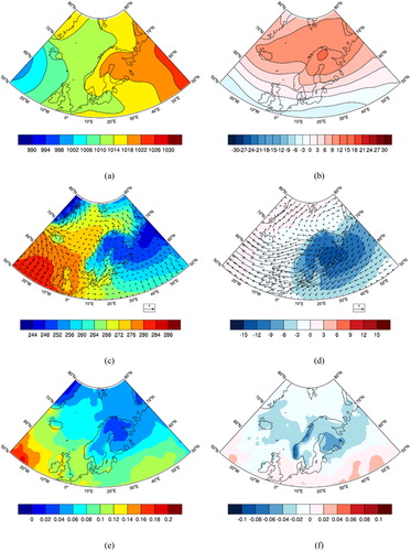
Figure 3 shows the composite results of the large-scale atmospheric state associated with widespread wintertime cold extremes. In the case of cold extremes, a high-pressure is located over Urals and Fennoscandia (Fig. 3a). The northern parts of the study region are affected by an anomalously high pressure and the southern parts by an anomalously low pressure (Fig. 3b). Over most of the study region up to 70^oN the wind is easterly (Fig. 3c). In winter, the air is climatologically colder in Siberia than in the central Arctic, which makes the easterly air-mass origin important, resulting in extremely cold winter events in Northern Europe. These are also favoured by negative anomalies in the cloud condensate content (vertical integral of cloud frozen water and cloud liquid water) (Fig. 3e,f), which result in reduced downward longwave radiation.

Fig. 3. Composites for all widespread cold extreme days of sea level pressure (a), its anomaly (b), 2-m air temperature and 10-m wind vector (c), their anomalies (d), vertically integrated cloud condensate content (e) and its anomaly (f).The units are hPa, °C, m/s and kg/m², respectively.

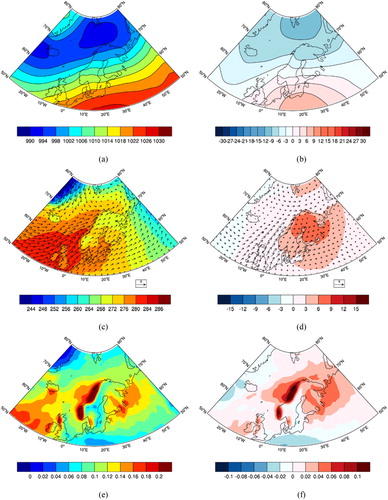
On the contrary, in the case of warm extremes (Fig. 4), a centre of low pressure anomaly is located over the Barents Sea and a centre of high pressure anomaly over Central Europe (Fig. 4b). The distribution of sea-level pressure (Fig. 4a) causes southwesterly winds to dominate over Northern Europe (Fig. 4c), bringing warm and humid air masses to contribute to extremely high temperatures in Northern Europe, especially in its northernmost parts (Fig. 4d). Besides, warm extremes are associated with strong positive anomalies in the cloud condensate content (Fig. 4e,f).

Fig. 4. As Fig. 3 but for the composites for all widespread warm extreme days.

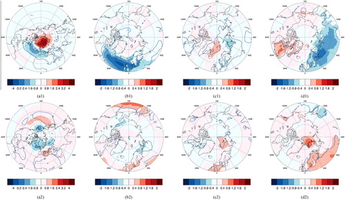
The spatial patterns of SLP corresponding to the cold extreme days (Fig. 5a1) were characterised by positive anomalies over the North Atlantic north of 60^oN, Barents Sea and Northern Europe, and negative anomalies in the North Atlantic from 30 to 50^oN, resembling the negative phase of NAO. On the contrary, the regression map of SLP corresponding to the warm extreme days (Fig. 5a2) shows negative anomalies north of 60^oN and positive anomalies in mid-latitudes. This pattern resembles the positive phase of the Arctic Oscillation (AO), although the negative anomalies in high latitudes are scattered. The regression maps of 10-m wind for extreme cold events show easterly wind anomalies over the North Atlantic, central and northern Europe and central Russia (Fig. 5b1), and the northerly wind anomalies over the Baltic Sea, eastern Barents Sea and Kara Sea (Fig. 5c1), which are favourable for the increased occurrence of extreme cold events over Northern Europe. The regression maps of 10-m wind for extreme warm events show westerly wind anomalies over the North Sea, Baltic Sea and surroundings and southerly winds over northwestern Europe and northern parts of Barents and Kara seas (Fig. 5c2), which are conducive to increase the occurrence of extreme warm events. The regression maps of downward longwave radiation fields for extreme cold and warm events are nearly opposite for Northern Europe (Fig. 5d1,d2). For extreme cold events, negative anomalies occur over Northern Europe and Russia (Fig. 5d1), but these regions have significant positive anomalies during extreme warm events.

Fig. 5. Regression maps of the sea level pressure (a1, a2), u10 (b1, b2), v10 (c1, c2) and downward longwave radiation (d1, d2) on the time series of the frequency of occurrence of extremely cold (upper row) and warm (lower row) events. The regions with blue line indicate results significant at 95% confidence level. The units are hPa, m/s, m/s and W/m², respectively. The regression coefficients shown as colour codes were calculated on the basis of the linear equation: y = a x + b, where y is the frequency of occurrence of warm/cold extremes, x is the explaining variable and a is the regression coefficient.

The results of regression analysis (Fig. 5) are basically consistent with those of composite analysis (Figs. 3 and 4). On this basis, we suggest that the temperature extremes in Northern Europe depend on the phases of SCA, NAO and AO, the direction of the surface wind as well as the cloud condensate content and downward longwave radiation. Easterly and northerly winds bring cold air masses from Siberia and central Arctic, while southwesterly flows transport warm, humid marine air masses from North Atlantic to Northern Europe, thus leading to the occurrence of the extreme temperature events.

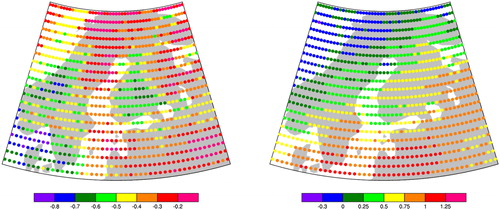
We further quantified the dependence of extreme temperatures on NAO by averaging the NAO index over days when cold and warm extremes occurred in each grid cell. The results demonstrated that to have an extremely cold winter day in Denmark, southern Sweden, southern Norway or the North Sea, a strongly negative NAO index (−0.6 to −0.9) was needed, on average, with some exceptions in mountainous inland regions (Fig. 6a). However, in the eastern and northern parts of our study region, extremely cold days did not require as negative NAO index; the mean values ranged from −0.1 to −0.4, except in southern and central Finland, where the range was from −0.4 to −0.7 (Fig. 6a). On the contrary, to have an extremely warm winter day in the southern and eastern parts of our study region, a strongly positive NAO index (typically from 0.5 to 1.5) was needed, whereas in the western and northern parts of the study region extremely warm temperatures were possible under slightly positive or even negative NAO index (Fig. 6b).

Fig. 6. Mean values of NAO index averaged over days when extremely cold (left) and warm days (right) occurred in each grid cell of ERA-Interim reanalysis.

3.3. SOM analyses

The SOM method was used here to classify the daily SLP anomaly patterns from winters 1979 to 2016 into 12 representative patterns in and around Northern Europe (Fig. 7). Among the 12 patterns, node 5 represents a low-pressure pattern whereas node 8 is a high-pressure pattern, and nodes 3 (eastern negative and western positive SLP anomaly) and 10 (eastern positive and western negative SLP anomaly) show dipole anomalies with opposite patterns. Other nodes represent transition states between the dipole anomalies and the cyclonic and anticyclonic patterns.

Fig. 7. Self-Organizing Maps (SOM) for wintertime (DJF) SLP anomaly for the 1979–2016 period. The blue and red numbers in the upper left corner of each SOM node denote number of extremely cold (blue) and warm days (red) that have occurred for the node. The numbers on top of each node mark the number of the node (1 to 12), its relative frequency of occurrence (in %) and the trend of the frequency of occurrence (day/yr). An asterisk (*) after the trend indicates results significant at 95% confidence level.

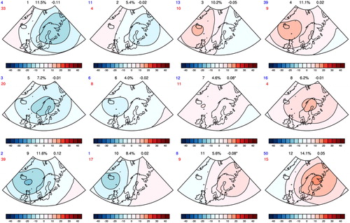
We show the frequency of occurrence and its trend for each SOM pattern and the number of extreme days corresponding to each pattern (Fig. 7). Nodes 1, 3, 4, 9 and 12 occur more than 10% of time, among which node 12 has the highest and node 9 the second-highest frequency of occurrence. In the case of nodes 4, 8 and, in particular, 12, Northern Europe is dominated by a high pressure anomaly, associated with a common occurrence of extremely cold events; 64% (105/165 days; blue numbers in Fig. 7) of the cold extremes are associated with these three nodes. On the contrary, in the case of nodes 1, 5 and 9 Northern Europe is covered by a strong low-pressure anomaly, and 51% (92/179 days; red numbers in Fig. 7) of the warm extremes are associated with these nodes.

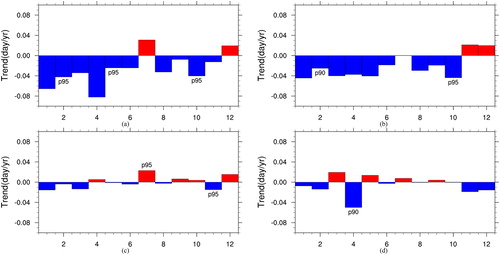
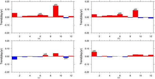
We next analyse the contributions of the 12 nodes to the trends in the frequency of occurrence of extreme warm/cold events in Northern Europe from the dynamic, thermodynamic and their interaction perspectives. In general, the frequency of occurrence of cold extremes has decreased (Fig. 8a), which is mostly due to increased temperatures in nodes 1–6 and 8–10, seen as the thermodynamic component reducing the occurrence of cold extremes (Fig. 8b). This trend is, however, opposed by decreased air temperatures of nodes 11 and 12 (Fig. 8b) and by increased occurrence of nodes 7 and 12, which are associated with a frequent occurrence of cold extremes (Fig. 8c). The interaction of dynamic and thermodynamic components is mostly reducing the occurrence of cold extremes (Fig. 8d). Considering the effect of all nodes taken together, the changes in thermodynamic processes explain 80.2% of the decreasing trend (−0.32 days/year) in the occurrence of cold extremes, followed by the changes in the interaction between thermodynamic and dynamic processes, which account for nearly 19.5% of the trend. The changes in dynamic processes only account for 0.3% of the trend. For the occurrence of warm extremes, the changes in thermodynamic processes also make the largest contribution, explaining 63.5% of the total trend. The second-largest contribution comes from interaction factors, which account for 37.4% of the trend, whereas the dynamic contributions only explain −0.9%, which offsets the contributions by the other two components. The total trend of the occurrence of extreme warm events is 0.34 day/year.

Fig. 8. The trend (day/yr) in the frequency of occurrence of extremely cold days for each SOM node during 1979–2016: (a) total trend, (b) thermodynamic contribution to the trend, (c) dynamic contribution and (d) interaction contribution. The number p95 (p90) indicate results significant at 95% (90%) confidence level.

Figure 9 presents the trends in the anomalies of SLP, downward long-wave radiation, 2-m air temperature and 10-m wind speed, and the composites of 2-m air temperature and 10-m wind in extreme cold cases of nodes 4, 7 and 12. We apply Eq. 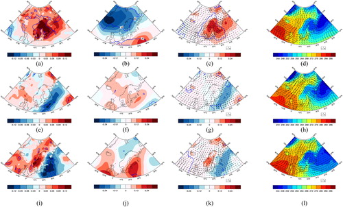(2)(2) $$\frac{dE}{dt}=\sum _{i=1}^K[\overline{f_i}\frac{d{E_i}^{\mathrm{\prime }}}{dt}+\overline{E_i}\frac{d{f_i}^{\mathrm{\prime }}}{dt}+\frac{d\left({E_i}^{\mathrm{\prime }}{f_i}^{\mathrm{\prime }}\right)}{dt}]$$(2) to analyse the contributions of the thermodynamic, dynamic and interaction components of each node to the trend in the occurrence of extreme temperatures. The largest contribution to the decreasing trend in the occurrence of cold extremes comes from the cold node 4, whereas the contributions of nodes 7 and 12 oppose the decreasing trend (Fig. 8a). In the case of node 4, the SLP anomaly is positive in Northern Europe (Fig. 7) but its trend is negative (Fig. 9b), that is, the high-pressure anomaly centred over Iceland has become weaker. In addition, the southwesterly wind and 2-m air temperature have increased in the study area (Fig. 9c), both of them reducing the occurrence of extreme cold events, so the contribution of the interaction component of node 4 is negative (Fig. 8d). The trend of SLP is positive for node 7 (Fig. 9f) but for node 12 it is negative over the Norwegian and Barents seas and positive farther south (Fig. 9j). Hence, the northeasterly (Fig. 9g) and northerly winds (Fig. 9k) have increased (although most grid points did not exhibit statistically significant trends), and the temperature has mostly decreased related to the increased occurrence of extremely cold events. Further, the temperature trend in node 12 is negative (Fig. 9l), and so the contribution of the thermodynamic component to the total trend of the occurrence of extremely cold events is positive (Fig. 8b).

Fig. 9. The trends of the downward longwave radiation anomaly (first column), sea level pressure anomaly (second column), 2-m air temperature and 10-m wind anomalies (third column) and the composites of 2-m air temperature and 10-m wind in extremely cold cases of node 4 (uppermost row), node 7 (middle row) and node 12 (lowermost row). The regions surrounded by a blue curve indicate results significant at 95% confidence level.

Similarly, we examined the contributions of each node to the occurrence of warm extremes (Fig. 10). The trend in the occurrence of warm extremes is positive (Fig. 10a), and mostly results from the thermodynamic component (Fig. 10b). The largest contribution to the total trend originates from node 9 (0.15 days/year), which is a warm node. It has become even warmer (Fig. 10b) and more common (Fig. 10c). Its thermodynamic and dynamic components account for 0.09 days/year and 0.04 days/year, respectively. As in the case of cold extremes, node 1 has the second-largest contribution to the trend of occurrence of warm extremes. For node 1, the interaction component gives the largest contribution to the trend, whereas the thermodynamic and dynamic components approximately offset each other.

Fig. 10. As Fig. 8, but for the extremely warm days.

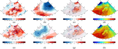
The trends in the anomalies of downward long-wave radiation, sea level pressure, 2-m air temperature and 10-m wind, and the composites of 2-m air temperature and 10-m wind are shown in Fig. 11 for the warm nodes 1 and 9. Compared with the SLP anomaly of nodes 1 and 9 (Fig. 7), the trends in Fig. 11b,f show that the centres of both low and high pressure have become stronger, strengthening the circulation patterns of these two nodes (although the trends in most areas are insignificant). Hence, the westerly (Fig. 11b,c) and southwesterly (Fig. 11f,g) winds have increased, contributing to the positive total trend. Downward long-wave radiation is an important factor for the contributions of the thermodynamic component. For example, the downward long-wave radiation has a strong increasing trend over the study region for node 4 (Fig. 9a) but a decreasing trend for node 12 when averaged over the study region (Fig. 9i), contributing to opposite thermodynamic components of the two nodes (Figs. 8b and 10b). Similarly, the downward long-wave radiation has increased for nodes 1 and 9 (Fig. 11), favouring the thermodynamic component of these nodes in decreasing the occurrence of cold extremes (Fig. 8b) and increasing the occurrence of warm extremes (Fig. 10b).

Fig. 11. As Fig. 9 but for extremely warm days for nodes 1 (upper row) and 9 (lower row).

It is not surprising that thermodynamic processes explained most of the trends in the occurrence of extremes. The net effect of the interaction component was to reduce the occurrence of cold extremes, in which it was more important than the dynamic component. Considering the effect of all nodes taken together, the interaction component accounted for 19% of the decreasing trend of cold extremes (−0.32 days/year). Moreover, the interaction component contributed to 37% of the increasing trend of warm extremes (0.34 days/year), again having a much larger effect than the dynamic component. In the case of cold extremes, node 4 had the strongest interaction component, which was significant at 90% confidence level (Fig. 8d; 90% criteria for confidence has been applied in several studies addressing atmospheric dynamics, e.g. Rudeva and Simmonds (2015) and Zahn et al. (2018)). For node 4, $E^{\mathrm{\prime }}$ and $f^{\mathrm{\prime }}$ (see Eq. (2)(2) $$\frac{dE}{dt}=\sum _{i=1}^K[\overline{f_i}\frac{d{E_i}^{\mathrm{\prime }}}{dt}+\overline{E_i}\frac{d{f_i}^{\mathrm{\prime }}}{dt}+\frac{d\left({E_i}^{\mathrm{\prime }}{f_i}^{\mathrm{\prime }}\right)}{dt}]$$(2) ) were mostly of the same sign from 1983 to 2003, and $E^{\mathrm{\prime }}{f}^{\mathrm{\prime }}$ was accordingly positive during these years (Fig. 12). However, from 2004 onwards $E^{\mathrm{\prime }}{f}^{\mathrm{\prime }}$ was on average negative, resulting in a negative trend of −0.05 days/year over the entire study period (despite of the negative values in 1979–1982). Focusing on the post-2003 changes, the negative trend in $E^{\mathrm{\prime }}{f}^{\mathrm{\prime }}$ was due to years 2008, 2011, 2012 and 2013. In 2008 and 2012, node 4 occurred frequently (positive $f^{\mathrm{\prime }}$) but under its occurrence extremely cold temperatures were uncommon (negative $E^{\mathrm{\prime }}$), resulting in a negative $E^{\mathrm{\prime }}{f}^{\mathrm{\prime }}.$ On the contrary, in years 2011 and 2013, node 4 seldom occurred but under its occurrence extremely cold temperatures were common, also resulting in a negative $E^{\mathrm{\prime }}{f}^{\mathrm{\prime }}.$

Fig. 12. Time series of $E,f,E^{\mathrm{\prime }},f^{\mathrm{\prime }}$ and $E^{\mathrm{\prime }}{f}^{\mathrm{\prime }}\mathrm{ }$ for node 4 in the case of cold extremes.

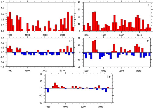
Considering warm extremes, only node 1 of the interaction component had a statistically significant (95%) trend (Fig. 10). Figure 13 shows that from 1979 to 2001, positive (negative) anomalies in the frequency of occurrence ($f^{\mathrm{\prime }}$) of node 1 were usually associated with negative (positive) anomalies in the frequency of extreme temperature occurrence ($E^{\mathrm{\prime }}$) under node 1, but from 2001 onward the situation was opposite. In winters 2005, 2008, 2009, 2010, 2012 and 2013 node 1 seldom occurred, and under its occurrence in winters 2005, 2010 and 2012 warm extremes seldom occurred, resulting in positive $E^{\mathrm{\prime }}{f}^{\mathrm{\prime }}.$ In winters 2006, 2014 and 2016, node 1 occurred frequently, and under its occurrence in 2006 and 2014 warm extremes were common, resulting in positive $E^{\mathrm{\prime }}{f}^{\mathrm{\prime }}$ for those winters. Accordingly, $E^{\mathrm{\prime }}{f}^{\mathrm{\prime }}$ had a positive trend over 1979–2016, indicating a positive interaction term for node 1.

Fig. 13. As Fig. 12 but for node 1 in the case of warm extremes.

Summarizing the results above, there seems not to be any coherent physical process responsible for the signs of the statistically significant interaction components. A lot of cases occurred even in successive years when a combination of negative $f^{\mathrm{\prime }}$ and positive $E^{\mathrm{\prime }}$ and a combination of positive $f^{\mathrm{\prime }}$ and negative $E^{\mathrm{\prime }}$ resulted in $E^{\mathrm{\prime }}{f}^{\mathrm{\prime }}$ of the same sign. Hence, we interpret that the interaction component mostly represented internal variability of the system.

4. Discussion

Using the daily ERA-interim reanalysis data and combining multiple methods (self-organizing maps, trend analysis, composite analysis and regression analysis), we studied the occurrence and drivers of wintertime temperature extremes in Northern Europe during 1979–2016. The main conclusions and findings of this study are as follows.

1. Cold extreme events occurred most frequently in winter 1984 (30 days) while warm extreme events occurred most frequently in winter 2006 (23 days). Although no significant decreasing trend has been detected in the occurrence of extremely cold events, a significant increasing trend was found in the occurrence of extremely warm events. Of all the extreme cold and warm days in the winters of 1979–2016 (DJF), less than a quarter were single-day events, and more than 58% of cold and 35% of warm extremes lasted for at least four days.

2. The result of composite and regression analyses suggest that the pattern of large-scale circulation, the direction of the surface wind and the cloud condensate content are among the important factors for the extremes. Widespread cold extremes were favoured by the Scandinavian Pattern and Ural Blocking, associated with advection of continental air-masses from the east, clear skies, and negative anomalies in downward longwave radiation. In the case of widespread warm extremes, centres of low pressure were typically located over the Barents Sea and west of Iceland, and a centre of high pressure over central Europe, which caused south-westerly winds to dominate over Northern Europe, bringing warm, cloudy air masses to northern Europe, especially to its northernmost parts. Strong positive (negative) anomalies in the cloud condensate content and downward longwave radiation were associated with warm (cold) extremes. As well known, the cold (warm) extremes are typically associated with the negative (positive) phase of NAO. For a cold extreme to occur in Denmark, southern Sweden and coastal regions of southern Norway, a strongly negative NAO was usually needed, and for a warm extreme to occur in Denmark, southern Sweden, the Baltic countries, northern Belarus north-western Russia, a strongly positive NAO was typically a prerequisite. In the northern parts of the study region, the role of NAO was smaller both in the case of cold and warm extremes. The cold extremes were closely associated with the Scandinavian Pattern and Ural Blocking, and the warm extremes with the Barents Sea low.

3. SLP anomaly fields were classified into 12 patterns applying the SOM method. The spatial patterns include cyclonic, anticyclonic and dipole anomalies and their transition states. The most common SOM nodes 12 (Scandinavian Pattern) and 9 (Icelandic Low) both showed a positive (although insignificant) trend in their frequency of occurrence (Fig. 7). Among days of cold (warm) extremes, node 12 (9) was the most common. Thermodynamic processes explained 80% (64%) of the decreasing (increasing) trend in the occurrence of extreme cold (warm) events. Considering occurrence of cold extremes, the largest contribution to the decreasing trend came from the cold node 4 (Icelandic high), which has become warmer. The frequency of occurrence of node 12 has increased, but the frequency of node 4 has decreased (insignificantly) and the contribution of node 4 to the decreasing occurrence of cold extremes is much larger than that of node 12. The contributions of thermodynamic and interaction components in node 4 account for most of the trend. The increasing of downward longwave radiation and south-westerly winds contribute to the decreasing occurrence of cold extremes. Considering the increased occurrence of widespread warm extremes, the largest contribution of the total trend came from node 9 (Icelandic low). The warming of the node and its increased occurrence accounted for 0.09 day/year and 0.04 day/year, respectively. We stress the difference between the SLP field most commonly associated with warm extremes (prominent Barents Sea low, Fig. 4a,b) and the factors primarily responsible for an increase in the occurrence of warm extremes: an overall increase in temperatures under most circulation patterns (Fig. 10b) and increased occurrence of the SLP anomaly with a strong Icelandic low (Fig. 7, node 9, and Fig. 10c). We note that even if the change in the occurrence of a node has not been significant, the change may still have remarkably affected the occurrence of extreme temperatures via the dynamic component, as in the case of nodes 1 and 9 for warm extremes (Fig. 10).

Although physical processes (such as heat transport and cloud radiative forcing) related to the most important nodes can be reasonably well understood, it is much more challenging to understand how large a portion of the changes observed was due to the climate warming trend and how much was due to internal decadal variability of the system. The thermodynamic component of the SOM analysis explained a large majority of the changes in the occurrence of extreme cold and warm events, and we assume that it is mostly driven by anthropogenic climate warming. It may include some contribution from the positive phase of the Atlantic Multi-decadal Oscillation (AMO, Zhang, 2015), but the AMO effect should be mostly present in the dynamic component. The AMO affects North Atlantic sea surface temperatures (Chylek et al., 2009), and these further affect European air temperatures, but mostly by generating anomalous atmospheric circulation patterns (O’Reilly et al., 2017), seen in the dynamic component, rather than directly affecting upstream conditions of marine air-masses advected to Europe (which represents a thermodynamic effect originating from a natural variability of the ocean, and should be reflected in the thermodynamic SOM component).

The interaction component accounted for 19% of the decreasing trend of cold extremes and 37% of the increasing trend of warm extremes. Although the interaction component is often assumed to result from systematic changes in physical interactions of dynamic and thermodynamic components of the climate system (e.g. Horton et al., 2015), our analyses suggest that the interaction component was mostly associated with chaotic variations. The dynamic component related to changes in atmospheric circulation probably represents both internal variability and forced responses to climate warming (see the paragraph below). In any case, the dynamic component only had a small contribution to the observed changes in extreme temperatures. Although the SOM method does not allow quantification of the contributions of forced and unforced changes, our results are qualitatively in line with McKinnon and Deser (2018), who stressed the non-negligible contribution of internal variability to warming trends in, among others, Scandinavia during the past 50 years.

Some of the changes that we observed were expected, such as the increased occurrence of the Scandinavian Pattern (Crasemann et al., 2017) and warming under the occurrence of most nodes. However, on the basis the decreased occurrence of the positive phase of NAO during winters 1979–2015 (Vihma et al., 2020), the increased occurrence of node 9, representing the Icelandic low, was not expected. In the case of positive NAO index, however, the low pressure centre is typically located farther west than in the case of node 9. It is also noteworthy that, although warm extremes have become significantly more common, the decrease in the occurrence of cold extremes is not statistically significant. This is related to factors that regionally act against the impacts of global warming: the increased occurrence of Scandinavian Pattern and decreased air temperatures under its occurrence. Scandinavian Pattern is often associated or merged with Ural Blocking (Peings, 2019), and the increasing occurrence of these patterns is probably not dominated by natural variability. According to model experiments of Crasemann et al. (2017), Arctic sea ice decline favours the occurrence of Scandinavian Pattern, and several papers have suggested that sea ice decline in the Barents and Kara seas favours Ural Blocking even with a positive feedback between the two (Inoue et al., 2012; Mori et al., 2014; Sato et al., 2014; Luo et al., 2016a, 2016b; Peings, 2019; Tyrlis et al., 2019; Cohen et al., 2020). An example of the combined effects of thermodynamic and dynamic processes is winter 2009/2010. It was a cold winter in Europe due to dynamic reasons, characterised by a very negative NAO index but, because of the general warming trend, it was much warmer than winters further in the past characterised by analogous large-scale circulation patterns (Cattiaux et al., 2010).

As a summary, we have analysed the influence of anomalies of sea-level pressure, downward long-wave radiation and 10-m wind on wintertime 2-m air temperature extremes in Northern Europe. Besides, variations in the surface conditions, such as the extent and thickness of sea ice and terrestrial snow pack, and in the surface fluxes of latent and sensible heat (Colfescu et al., 2016) can affect local air temperatures (Sousa et al., 2018; Ye and Wu, 2017). Further work is needed on the impact of these factors on the surface temperature and air-surface heat exchange. The SOM method applied allows attribution of the observed changes to thermodynamic and dynamic forcing factors, but major challenges remain in separation of the changes in forced responses to drivers of the climate system and the underlying internal variability of the system. In this respect, a promising way forward is the use of artificial intelligence in analyses of climate data (Barnes et al., 2019).

Acknowledgement

We thank the European Centre for Medium-Range Weather Forecasts (ECMWF) for the ERA-Interim reanalysis data (downloaded from https://www.ecmwf.int/en/forecasts/datasets/reanalysis-datasets/era-interim).

Disclosure statement

No potential conflict of interest was reported by the authors.

Additional information

Funding

This work was supported by National Key R&D Program of China (Grant nos. 2018YFC1505806, 2018YFC1505802), the National Natural Science Foundation of China 41976221 and 41576029, Beijing Municipal Natural Science Foundation (Grant no. 8182023), National Key R&D Program of China (Grant no. 2017YFE0111700), the Academy of Finland (contract 317999) and the China Scholarship Council fellowship no. 201904180014.

References

- Barnes, E. A., Hurrell, J. W., Ebert-Uphoff, I., Anderson, C. and Anderson, D. 2019. Viewing forced climate patterns through an AI Lens. Geophys. Res. Lett. 46, 13389–13398. doi:10.1029/2019GL084944
- Beniston, M., Stephenson, D. B., Christensen, O. B., Ferro, C. A. T., Frei, C. and co-authors. 2007. Future extreme events in European climate: an exploration of regional climate model projections. Clim. Change 81, 71–95. doi:10.1007/s10584-006-9226-z
- Cassano, E. N., Cassano, J. J. and Nolan, M. 2011. Synoptic weather pattern controls on temperature in Alaska. J. Geophys. Res. 116, D11108. doi:10.1029/2010JD015341
- Cassano, J. J., Cassano, E. N., Seefeldt, M. W., Gutowski, W. J., Glisan, J. M. and co-authors. 2016. Synoptic conditions during wintertime temperature extremes in Alaska. J. Geophys. Res. Atmos. 121, 3241–3262. doi:10.1002/2015JD024404
- Cassano, E. N., Lynch, A. H., Cassano, J. J. and Koslow, M. R. 2006. Classification of synoptic patterns in the western Arctic associated with extreme events at Barrow, Alaska, USA. Clim. Res. 30, 83–97. doi:10.3354/cr030083
- Cassano, J. J., Uotila, P., Lynch, A. H. and Cassano, E. N. 2007. Predicted changes in synoptic forcing of net precipitation in large Arctic river basins during the 21st century. J. Geophys. Res. 112, 1–20.
- Cattiaux, J., Vautard, R., Cassou, C., Yiou, P., Masson‐Delmotte, V. and co-authors. 2010. Winter 2010 in Europe: a cold extreme in a warming climate. Geophys. Res. Lett. 37.
- Chylek, P., Folland, C. K., Lesins, G., Dubey, M. K. and Wang, M. 2009. Arctic air temperature change amplification and the Atlantic Multidecadal Oscillation. Geophys. Res. Lett. 36, L14801. doi:10.1029/2009GL038777
- Cohen, J., Zhang, X., Jung, T., Kwok, R., Overland, J. and co-authors. 2020. Divergent consensuses on Arctic amplification influence on midlatitude severe winter weather. Nat. Clim. Change 10, 20–29. doi:10.1038/s41558-019-0662-y
- Colfescu, I., Hegerl, G. and Tett, S. 2016. Evaluation of mechanisms of extreme temperatures over Europe[C]. In: EGU General Assembly Conference Abstracts 18. Vienna, Austria.
- Comas-Bru, L. and McDermott, F. 2014. Impacts of the EA and SCA patterns on the European twentieth century NAO–winter-climate relationships. QJR. Meteorol. Soc. 140, 354–363. 2158. doi:10.1002/qj.2158
- Crasemann, B., Handorf, D., Jaiser, R., Dethloff, K., Nakamura, T. and co-authors. 2017. Can preferred atmospheric circulation patterns over the North-Atlantic-Eurasian region be associated with Arctic sea ice loss? Polar Sci. 14, 9–20. doi:10.1016/j.polar.2017.09.002
- Dee, D. P., Uppala, S. M., Simmons, A. J., Berrisford, P., Poli, P. and co-authors 2011. The ERA-Interim reanalysis: configuration and performance of the data assimilation system. QJR. Meteorol. Soc. 137, 553–597. doi:10.1002/qj.828
- Deser, C., Hurrell, J. W. and Phillips, A. S. 2017. The role of the North Atlantic oscillation in European climate projections. Clim. Dyn. 49(9-10): 3141–3157.
- Deser, C., Sun, L., Tomas, R. A. and Screen, J. 2016. Does ocean coupling matter for the northern extratropical response to projected Arctic sea ice loss? Geophys. Res. Lett. 43, 2149–2157. doi:10.1002/2016GL067792
- Gibson, P. B., Uotila, P., Perkins-Kirkpatrick, S. E., Alexander, L. V., Pitman, A. J. and co-authors 2016. Evaluating synoptic systems in the CMIP5 climate models over the Australian region. Clim. Dyn. 47, 2235–2251. doi:10.1007/s00382-015-2961-y
- Graham, R. M., Cohen, L., Petty, A. A., Boisvert, L. N., Rinke, A. and co-authors. 2017. Increasing frequency and duration of Arctic winter warming events. Geophys. Res. Lett. 44, 6974–6983. doi:10.1002/2017GL073395
- Hanna, E., Hall, R. J., Cropper, T. E., Ballinger, T. J., Wake, L. and co-authors. 2018. Greenland blocking index daily series 1851-2015: analysis of changes in extremes and links with North Atlantic and UK climate variability and change. Int. J. Climatol.
- Horton, D. E., Johnson, N. C., Singh, D., Swain, D. L., Rajaratnam, B. and co-authors. 2015. Contribution of changes in atmospheric circulation patterns to extreme temperature trends. Nature 522, 465–469. doi:10.1038/nature14550
- Hurrell, J. W. and Deser, C. 2009. North Atlantic climate variability: the role of the North Atlantic Oscillation. J. Mar. Syst. 78, 28–41. doi:10.1016/j.jmarsys.2008.11.026
- Inoue, J., Hori, M. E. and Takaya, K. 2012. The role of Barents Sea ice in the wintertime cyclone track and emergence of a warm‐Arctic cold‐Siberian anomaly. J. Clim. 25, 2561–2568. doi:10.1175/JCLI-D-11-00449.1
- Instanes, A., Kokorev, V., Janowicz, R., Bruland, O., Sand, K. and co-authors. 2016. Changes to freshwater systems affecting Arctic infrastructure and natural resources. J. Geophys. Res. Biogeosci. 121, 567–585. doi:10.1002/2015JG003125
- Jaagus, J., Briede, A., Rimkus, E. and Remm, K. 2014. Variability and trends in daily minimum and maximum temperatures and in the diurnal temperature range in Lithuania, Latvia and Estonia in 1951-2010. Theor. Appl. Climatol. 118, 57–68. doi:10.1007/s00704-013-1041-7
- Johnson, N. C., Feldstein, S. B. and Tremblay, B. 2008. The continuum of northern hemisphere teleconnection patterns and a description of the NAO shift with the use of self-organizing maps. J. Clim. 21, 6354–6371. doi:10.1175/2008JCLI2380.1
- Kim, B.-M., Son, S.-W., Min, S.-K., Jeong, J.-H., Kim, S.-J. and co-authors. 2014. Weakening of the stratospheric polar vortex by Arctic sea-ice loss. Nat. Commun. 5, 4646. doi:10.1038/ncomms5646
- Kivinen, S., Rasmus, S., Jylhä, K. and Laapas, M. 2017. Long-term climate trends and extreme events in Northern Fennoscandia (1914–2013). Climate 5, 16. doi:10.3390/cli5010016
- Kodra, E. and Ganguly, A. R. 2014. Asymmetry of projected increases in extreme temperature distributions. Sci. Rep. 4, 5884.
- Kohonen, T. 2001. Self-Organizing Maps. Springer, Berlin, 501 p.
- Lim, Y.-K. 2015. The East Atlantic/West Russia (EA/WR) teleconnection in the North Atlantic: climate impact and relation to Rossby wave propagation. Clim. Dyn. 44, 3211–3222.. doi:10.1007/s00382-014-2381-4
- Loikith, P. C. and Broccoli, A. J. 2015. Comparison between observed and model-simulated atmospheric circulation patterns associated with extreme temperature days over North America using CMIP5 historical simulations. J. Clim. 28, 2063–2079. doi:10.1175/JCLI-D-13-00544.1
- Luo, D., Xiao, Y., Diao, Y., Dai, A., Franzke, C. L. E. and co-authors. 2016b. Impact of Ural blocking on winter warm Arctic-cold Eurasian anomalies. Part II: the link to the North Atlantic Oscillation. J. Clim. 29, 3949–3971. doi:10.1175/JCLI-D-15-0612.1
- Luo, D., Xiao, Y., Yao, Y., Dai, A., Simmonds, I. and co-authors. 2016a. Impact of Ural blocking on winter warm Arctic-cold Eurasian anomalies. Part I: blocking induced amplification. J. Clim. 29, 3925–3947. doi:10.1175/JCLI-D-15-0611.1
- Marshall, J., Johnson, H. and Goodman, J. 2001. A study of the interaction of the North Atlantic Oscillation with ocean circulation. J. Clim. 14, 1399–1421. doi:10.1175/1520-0442(2001)014<1399:ASOTIO>2.0.CO;2
- Marshall, J., Kushnir, Y., Battisti, D., Chang, P., Czaja, A. and co-authors. 2001. North Atlantic climate variability: phenomena, impacts and mechanisms. Int. J. Climatol. 21, 1863–1898. doi:10.1002/joc.693
- Matthes, H., Rinke, A. and Dethloff, K. 2015. Recent changes in Arctic temperature extremes: warm and cold spells during winter and summer. Environ. Res. Lett. 10, 114020. doi:10.1088/1748-9326/10/11/114020
- McKinnon, K. A. and Deser, C. 2018. Internal variability and regional climate trends in an observational large ensemble. J. Clim. 31, 6783–6802. doi:10.1175/JCLI-D-17-0901.1
- Mori, M., Watanabe, M., Shiogama, H., Inoue, J. and Kimoto, M. 2014. Robust Arctic sea‐ice influence on the frequent Eurasian cold winters in past decades. Nat. Geosci. 7, 869–873.. doi:10.1038/ngeo2277
- Nakamura, T., Yamazaki, K., Iwamoto, K., Honda, M., Miyoshi, Y. and co-authors. 2015. A negative phase shift of the winter AO/NAO due to the recent Arctic sea-ice reduction in late autumn. J. Geophys. Res. Atmos. 120, 3209–3227. doi:10.1002/2014JD022848
- Nygård, T., Graversen, R. G., Uotila, P., Naakka, T. and Vihma, T. 2019. Strong dependence of wintertime Arctic moisture and cloud distributions on atmospheric large-scale circulation. J. Clim. 32, 8771–8790. doi:10.1175/JCLI-D-19-0242.1
- O’Reilly, C. H., Woollings, T. and Zanna, L. 2017. The dynamical influence of the Atlantic multidecadal oscillation on continental climate. J. Clim. 30, 7213–7230.. doi:10.1175/JCLI-D-16-0345.1
- Overland, J., Francis, J., Hall, R., Hanna, E., Kim, S.-J. and co-authors. 2015. The Melting Arctic and Mid-latitude weather patterns: are they connected? J. Clim. 28, 7917–7932. doi:10.1175/JCLI-D-14-00822.1
- Peings, Y. 2019. Ural blocking as a driver of early‐winter stratospheric warmings. Geophys. Res. Lett. 46, 5460–5468. doi:10.1029/2019GL082097
- Räisänen, J. 2019. The effect of atmospheric winds on recent temperature changes in Finland. Ilmastokatsaus.
- Räisänen, J. and Ruokolainen, L. 2008. Ongoing global warming and local warm extremes: a case study of winter 2006-2007 in Helsinki, Finland. Geophysica 44.
- Rudeva, I. and Simmonds, I. 2015. Variability and trends of global atmospheric frontal activity and links with large-scale modes of variability. J. Clim. 28, 3311–3330.. doi:10.1175/JCLI-D-14-00458.1
- Rutgersson, A., Jaagus, J., Schenk, F., Stendel, M.,Bärring, L., and co-authors 2015. The BACC II Author Team (Ed.). Recent change—atmosphere. In: Second Assessment of Climate Change for the Baltic Sea Basin. Regional Climate Studies. Springer, Cham. 69–97.
- Sato, K., Inoue, J. and Watanabe, M. 2014. Influence of the Gulf Stream on the Barents Sea ice retreat and Eurasian coldness during early winter. Environ. Res. Lett. 9, 084009.. doi:10.1088/1748-9326/9/8/084009
- Screen, J. A., Deser, C., Simmonds, I. and Tomas, R. 2014. Atmospheric impacts of Arctic sea-ice loss, 1979-2009: separating forced change from atmospheric internal variability. Clim. Dyn. 43, 333–344. doi:10.1007/s00382-013-1830-9
- Screen, J. A. and Simmonds, I. 2014. Amplified mid-latitude planetary waves favour particular regional weather extremes. Nat. Clim. Change 4, 704–709. doi:10.1038/nclimate2271
- Shepherd, T. 2014. Atmospheric circulation as a source of uncertainty in climate change projections. Nat. Geosci. 7, 703–708.. doi:10.1038/ngeo2253
- Shepherd, T. G. 2015. Climate science: the dynamics of temperature extremes. Nature 522, 425–427.. doi:10.1038/522425a
- Shevnina, E., Silaev, A. and Vihma, T. 2019. Probabilistic projections of annual runoff and potential hydropower production in Finland. UJG. 7, 43–55. doi:10.13189/ujg.2019.070201
- Sillmann, J., Thorarinsdottir, T., Keenlyside, N., Schaller, N., Alexander, L. V. and co-authors. 2017. Understanding, modeling and predicting weather and climate extremes: challenges and opportunities. Weather Clim. Extremes 18, 65–74.. doi:10.1016/j.wace.2017.10.003
- Smith, D., Dunstone, N. J., Scaife, A. A., Fiedler, E. K., Copsey, D. and co-authors. 2017. Atmospheric response to Arctic and Antarctic sea ice: the importance of ocean-atmosphere coupling and the background state. J. Clim. 30, 4547–4565. doi:10.1175/JCLI-D-16-0564.1
- Sousa, P. M., Trigo, R. M., Barriopedro, D., Soares, P. M. M., Santos, J. A. and co-authors 2018. European temperature responses to blocking and ridge regional patterns. Clim. Dyn. 50, 457–477. doi:10.1007/s00382-017-3620-2
- Steiger, R., Scott, D., Abegg, B., Pons, M. and Aall, C. 2019. A critical review of climate change risk for ski tourism. Curr. Issues Tourism 22, 1343–1379. doi:10.1080/13683500.2017.1410110
- Tuomenvirta, H., Alexandersson, H., Drebs, A., Frich, P., Nordli, P. O. and co-authors . 2000. Trends in Nordic and Arctic temperature extremes and ranges. J. Clim. 13, 977–990. doi:10.1175/1520-0442(2000)013<0977:TINAAT>2.0.CO;2
- Tyrlis, E., Manzini, E., Bader, J., Ukita, J., Nakamura, H. and co-authors. 2019. Ural blocking driving extreme Arctic sea ice loss, cold Eurasia, and stratospheric vortex weakening in autumn and early winter 2016–2017. J. Geophys. Res. 124..
- Vavrus, S. J. 2018. The influence of arctic amplification on mid-latitude weather and climate. Curr. Clim. Change Rep. 4, 238–249. doi:10.1007/s40641-018-0105-2
- Vihma, T. 2017. Weather extremes linked to interaction of the Arctic and mid-latitudes. In: Climate Extremes: Mechanisms and Potential Prediction. Geophysical Monograph Series (ed. S.-Y. Wang J.-H. Yoon, C. C. Funk, and R. R. Gillies) Vol. 226, American Geophysical Union, 418 pp.
- Vihma, T., Graversen, R., Chen, L., Handorf, D., Skific, N. and co-authors. 2020. Effects of the tropospheric large-scale circulation on European winter temperatures during the period of amplified Arctic warming. Int. J. Climatol. 40, 509–529. doi:10.1002/joc.6225
- Vikhamar-Schuler, D., Isaksen, K., Haugen, J. E., Tømmervik, H., Luks, B. and co-authors . 2016. Changes in winter warming events in the Nordic Arctic region. J. Clim. 29, 6223–6244. doi:10.1175/JCLI-D-15-0763.1
- Vors, L. S. and Boyce, M. S. 2009. Global declines of caribou and reindeer. Global Change Biol. 15, 2626–2633.. doi:10.1111/j.1365-2486.2009.01974.x
- Walsh, J. E., Phillips, A. S., Portis, D. H. and Chapman, W. L. 2001. Extreme cold outbreaks in the United States and Europe, 1948-99. J. Clim. 14, 2642–2658. doi:10.1175/1520-0442(2001)014<2642:ECOITU>2.0.CO;2
- Wrona, F. J., Johansson, M., Culp, J. M., Jenkins, A., Mård, J. and co-authors. 2016. Transitions in Arctic ecosystems: ecological implications of a changing hydrological regime. J. Geophys. Res. Biogeosci. 121, 650–674. doi:10.1002/2015JG003133
- Yang, Z., Hanna, E., Callaghan, T. V. and Jonasson, C. 2012. How can meteorological observations and microclimate simulations improve understanding of 1913–2010 climate change around Abisko, Swedish Lapland? Met. Apps. 19, 454–463. doi:10.1002/met.276
- Ye, K. and Wu, R. 2017. Autumn snow cover variability over northern Eurasia and roles of atmospheric circulation. Adv. Atmos. Sci. 34, 847–858. doi:10.1007/s00376-017-6287-z
- Yu, L., Yang, Q., Vihma, T., Jagovkina, S., Liu, J. and co-authors 2018. Features of extreme precipitation at Progress station, Antarctica. J. Clim. 31, 9087–9105. doi:10.1175/JCLI-D-18-0128.1
- Zahn, M., Akperov, M., Rinke, A., Feser, F. and Mokhov, I. I. 2018. Trends of cyclone characteristics in the Arctic and their patterns from different reanalysis data. J. Geophys. Res. Atmos. 123, 2737–2751.. doi:10.1002/2017JD027439
- Zhang, R. 2015. Mechanisms for low-frequency variability of summer Arctic sea ice extent. Proc. Natl. Acad. Sci. USA 112, 4570–4575. doi:10.1073/pnas.1422296112