On the contribution of internal climate variability to European future climate trends

Abstract

Large historical and future ensemble simulations from the Max-Planck Institute and the Canadian Earth System Models and from CMIP5 have been analysed to investigate the uncertainty due to internal variability in multi-decadal temperature and precipitation trends over Europe. Internal variability dominates the uncertainties in temperature and precipitation trends in all seasons at 30-year time scales. Locally, seasonal 30-year temperature trends deviate up to ±3 °C from the ensemble mean trend. Thus, in the entire of Europe, local seasonal temperature changes until year 2050 from below −1 °C up to more than 4 °C are possible according to the model results. Up to 30% of all ensemble members show negative temperature trends until year 2050 in winter, up to 10% of the members in summer. Uncertainties of 30-year precipitation trends due to internal variability exceed the trends almost everywhere in Europe. Only in few European regions more than 75% of the members agree on the sign of the change until year 2050. In southern Sweden, minimum and maximum winter (summer) temperature trends in the next 30 years differ with up to 7 °C (5 °C) between individual members of the large model ensembles. Large positive temperature trends are linked to positive (negative) precipitation trends in winter (summer) in southern Sweden. This variability is attributed to the variability in large scale atmospheric circulation trends, mainly due to internal atmospheric variability. We find only weak linkages between the variability of temperature trends and the dominant decadal to multi-decadal climate modes. This indicates that there is limited potential to predict the multi-decadal variability in climate trends. The main findings from our study are robust across the large ensembles from the different models used in this study but at the local scale, the results depend also on the choice of the model.

Keywords:

• internal climate variability
• European future climate trends
• uncertainties of trends
• variability in southern Sweden
• large ensemble global model simulations

1. Introduction

Climate projections show large uncertainties in future trends (Knutti and Sedlacek, 2013). The uncertainties are normally linked to three main sources: uncertainties in emission scenarios, or more general in external forcings, model errors, and internal variability (Hawkins and Sutton, 2009). Uncertainties in the future climate change due to uncertain emission scenarios can not be reduced as long as the world’s countries have not agreed on, and showed their capability and willingness to follow international agreements.

Uncertainties due to model errors are often addressed with the use of multi-model ensembles, such as the simulations performed in Coupled Model Intercomparison Projects (CMIP). This approach assumes that models do not have common shortcomings, which would lead to the same erroneous response of all models to future emission forcing.

The third source, internal variability has increasingly received attention in recent years. Analyses of large ensemble simulations with single models have shown that internal variability has often been underestimated and that it contributes to future climate change at time-scales up to several decades, especially at the regional level (Hawkins and Sutton, 2009; Hawkins, 2011; Hawkins and Sutton, 2012; Deser et al., 2014; von Trentini et al., 2019). Fischer et al. (2014) showed that the disagreement of temperature and precipitation extremes between individual model simulations primarily arises from internal variability, whereas models agree well on the forced signal.

Results from large ensemble simulations with the CCSM3 model indicate that internal atmospheric variability connected with annular modes of circulation variability is the largest source for uncertainties in middle and high latitudes and that a large number of ensemble members is necessary to statistically distinguish trends in precipitation and atmospheric circulation from internal variability (Deser, Phillips et al., 2012). Similarly, Horton et al. (2015) showed that observed atmospheric circulation trends are the main driver of many observed climate trends and of trends in extremes. A recent study by Dai and Bloecker (2019) using the CCSM large ensemble (CCSM-LENS) and the CanESM2 large ensembles (CanESM2-LENS) identified the Inter-decadal Pacific Oscillation and Arctic sea ice as main sources for internal climate variability. Rondeau-Genesse and Braun (2019) analysed the role of internal variability for future warming based on CCSM-LENS and CanESM2-LENS and found that ensemble members with a slowdown of warming in 2021–2040 show a strongly increased likelihood for very fast warming in the following decades.

Internal variability has further been linked to large uncertainty in the timing of future Arctic summer sea ice loss (Jahn et al., 2016; Niederdrenk and Notz, 2018). Kirchmeier-Young et al. (2017) used the CanESM2-LENS and showed that the sea ice minimum 2012 would have been very unlikely without anthropogenic influence. Suárez-Gutiérrez et al. (2018) analysed internal variability at 1.5 °C and 2 °C of global warming in the MPI-ESM-Grand Ensemble (MPI-ESM-GE) and found that the internal variability in European summers is much larger than at the global level. A recent study from Bengtsson and Hodges (2019) used the historical simulations of the MPI-ESM-GE to show that both global and regional observed multi-decadal anomalies of two metre air temperature (T2m) were significantly affected by internal variability. Marotzke (2019) found that internal variability masks most of the effects of an efficient implementation of the Paris Agreement until year 2035.

Uncertainties to internal variability are largest at the local level (Hawkins, 2011; Deser, Knutti et al., 2012). Long-term station observations at different places across Europe show large internal variability of temperature (Moberg et al., 2000). Observations from Uppsala in Sweden, Europe’s longest continuous temperature time-series, show that 30-year mean winter temperature varies by several degrees between different observed 30-year periods (Moberg and Bergström, 1997). The future climate of the real world will not follow the ensemble means of models. Each realisation of a model ensemble is an equally likely realisation of the future climate, assuming given future external forcings. Thus, to better cover the range of possible future climate paths, adaptation actions need to consider the outcomes from large ensembles of climate simulations and manage the connected uncertainties.

In this study, we use two different large model ensembles (MPI-ESM-GE and CanESM2-LENS) and compare them to multi-model ensembles of CMIP5-models. We investigate the uncertainty of local temperature and precipitation trends due to internal variability for two different future time periods (2021–2050 and 2021–2100). We analyse the contribution of this internal variability to the full uncertainty in CMIP5-model ensembles using two different scenarios (RCP4.5 and RCP8.5). Our analysis focuses in particular on the region of southern Sweden and we investigate the main drivers for the internal variability in this region to explore potential predictors for the regional future climate trends.

2. Data and method

2.1. Observations and reanalysis data

We use the long observed temperature record from Uppsala (Sweden) since 1722 (Moberg and Bergström, 1997) and ERA-interim reanalysis data (Dee et al., 2011). The observational data are used as comparison to the trends and their variations in the model results. Note, that observations and reanalyses can only provide rough estimates of the variations of trends due to internal variability since they are comparably short and stem from a climate in transition with changing and varying external forcing parameters.

2.2. Model simulations

An overview of the model simulations that we use in this study is provided in Table 1. More specifically we use the following simulations:

Table 1. Model simulations used for the analysis.

Ensemble	Time-period	Number of members
MPI-ESM-GE	1850–2100 Hist + RCP4.5	100
CanESM2-LENS	1950–2100 Hist + RCP8.5	50
CMIP5	1850–2100 Hist + RCP4.5 + RCP8.5	34 in total, 1 member per model: ACCESS1-0, ACCESS1-3, BCC-CSM1-1, CanESM2, CCSM4, CMCC-CM, CMCC-CMS, CNRM-CM5, CSIRO-Mk3-6-0, EC-EARTH, FGOALS-g2, FIO-ESM, GFDL-CM3, GFDL-ESM2G, GFDL-ESM2M, GISS-E2-H, GISS-E2-R-CC, GISS-E2-R, HadCM3, HadGEM2-AO, HadGEM2-CC, HadGEM2-ES, INMCM4_ESM, IPSL-CM5A-LR, IPSL-CM5A-MR, IPSL-CM5B-LR, MIROC5, MIROC-ESM-CHEM, MIROC-ESM, MPI-ESM-LR, MPI-ESM-MR, MRI-CGCM3, NorESM1-ME, NorESM1-M

2.2.1. Max Planck Institute Earth System Model Grand Ensemble (MPI-ESM-GE)

The MPI-ESM-GE (Maher et al., 2019) consists of an ensemble of 100 historical simulations (1850–2005) extended to the future (2006–2100) following different Representative Concentration Pathways (RCP2.6, RCP4.5, RCP8.5) and the 1% CO₂ scenarios of CMIP5 (Taylor et al., 2012). The MPI-ESM-GE uses the low resolution configuration of MPI-ESM version 1.1, which is an updated version of the one used for the Coupled Model Intercomparison Project Phase 5 (CMIP5). MPI-ESM consists of the atmosphere model ECHAM6 and the ocean-sea ice model MPIOM. ECHAM6 has a spectral horizontal resolution of T63 (ca 1.88°) and 47 vertical layers. MPIOM has a formal resolution of 1.5° and 40 vertical layers.

Evaluations of the CMIP5 version are provided by Giorgetta et al. (2013) for the atmosphere, Jungclaus et al. (2013) for the ocean and Notz et al. (2013) for the sea ice. The MPI-ESM-GE has been used in a number of recent studies (Bittner et al., 2016; Hedemann et al., 2017; Suárez-Gutiérrez et al., 2017; Niederdrenk and Notz, 2018; Bengtsson and Hodges, 2019).

When performing our analysis only the historical and the RCP2.6 and RCP4.5 future simulations of the MPI-ESM-GE were available. Thus, we do not discuss the RCP8.5 scenario in this study. In the result section, we discuss only the historical and the RCP4.5 simulations. The results from the RCP2.6 simulations lead to the same conclusions concerning uncertainties due to internal variability as the RCP4.5 simulations and are thus not further discussed.

2.2.2. Canadian Earth System Model-Large Ensemble (CanESM2-LENS)

The CanESM2-LENS (Sigmond and Fyfe, 2016) consists of an ensemble of 50 members covering the period 1950–2100. Until 2005, the simulations were run using CMIP5 historical forcings. Thereafter, forcings followed the RCP8.5 emission scenario. The ensemble is based on the five members of CMIP5 historical simulations with CanESM2 (Arora et al., 2011) performed by the Canadian Centre for Climate Modelling and Analysis. In 1950, from each of the five members, initial conditions were perturbed (by changing the seed of a random number generator in the cloud parameterization) to start 10 new members, resulting in total 50 members. The second generation Canadian Earth System Model (CanESM2) consists of the physical coupled atmosphere-ocean model CanCM4, the terrestrial carbon model CTEM (Arora, 2003) and the ocean carbon model CMOC (Christian et al., 2010). The CanESM2-LENS was proposed by the Canadian Sea Ice and Snow Evolution Network (CanSISE) Climate Change and Atmospheric Research (CCAR) Network project, which also coordinated much of the initial analysis of the large ensembles. A detailed description of CanESM2-LENS is provided by Kirchmeier-Young et al. (2017).

2.2.3. Cmip5-model ensemble (CMIP5)

Historical and future simulations following RCP4.5 and RCP8.5 from 34 CMIP5 models are used for the analysis in this study. We use ensemble member 1 from each of the models (see Table 1). Note, that several modelling centres provided simulations with different model versions. These are treated as individual models in the analysis since they often differ from each other substantially and it would not be straightforward to decide which one of the different model versions to use.

2.3. Methods

To analyse the variability of temperature and precipitation trends, we calculate standard deviations across model members at the grid point scale, analyse maximum and minimum trends and probability distributions. For MPI-ESM-GE and CanESM2-LENS, this provides us clear measures for the contribution of the internal variability to uncertainties of trends at different time-scales.

The CMIP5 ensemble includes both uncertainties due to internal variability and due to different model biases. Thus, from the CMIP5 ensemble, it is not possible to access the uncertainty due to internal variability alone. The CMIP5 ensemble is used here as comparison to the trends and their uncertainties in the single model large ensembles and to investigate how much of the spread in the CMIP5-ensemble might be explained by internal variability.

All data sets were remapped to a common 1° × 1° degree grid before calculating any trends or standard deviations.

The analysis will mainly focus on 30-year trends and their uncertainty as 30 years is the WMO (World Meteorological Organizations) standard time scale for climatological means. Further, the period until 2050, often called ‘the near future’, is about 30 years from now. As a first step, we analyse the period 1985–2014. Thereafter, we focus on the near future period 2021–2050 followed by the far future period 2021–2100.To calculate significances of correlations, we applied a two-sided Student’s t-test (von Storch and Zwiers, 1999). The trends are calculated using a linear least squares approach. Here, we are deliberately not calculating significances for the trends in the ensemble means or the individual members. The aim of this study is to analyse the uncertainties of trends and their entire possible range as depicted by the large ensembles and not if a trend is significant. The real future will not follow the ensemble mean of models but each single ensemble member is an as likely future outcome. Thus, each single member is as relevant for decision makers and stakeholders and it is not of importance if ensemble mean trend is significant or not.

3. Results

3.1. Uncertainties in recent temperature and precipitation trends

Figures 1 and 2 show the T2m and P trends in the ERA-interim data and of the model ensemble means between 1985 and 2014. Winter temperature increases in most of Europe with the warming over northern and southeastern parts of Europe reaching up to 3 °C per 30 years. In the very east of Europe, negative trends can be identified and T2m decreases by 2 °C in the regions of the Ural-mountains. This has been linked by several studies to the recent sea ice reduction (e.g. Mori et al., 2014; Vihma, 2014) but could also be due to internal variability (Ogawa et al., 2018; Koenigk et al., 2019). In addition, parts of southwestern Europe show a cooling between 1985 and 2014. Variations of winter T2m trends are high on rather small spatial scales in ERA-interim. In contrast, the model ensemble means show much smoother spatial trend patterns in winter as expected. All three sets of ensemble simulations agree on the trend patterns with largest warming over northeastern Europe and smaller warming trends towards the southwest of the continent (Fig. 1b–d). The trends are largest in CanESM2-LENS. While parts of the observed trend pattern, particularly the strong warming in the north and small trends in the southwest, are reproduced by the models, none of the model ensemble means show any negative trend over any region in Europe. However, spatial variations of the trend in individual model members can be as large as in the reanalysis data (Fig. 1i–l) and single members can show completely different trends compared to the ensemble mean (Fig. 1j,k).

Fig. 1. Winter (DJF average) and summer (JJA average) two-meter air temperature (T2m) trends in ERA-interim data (a, e), the ensemble means of MPI-ESM-GE (b, f), CanESM2-LENS (c, g) and CMIP5 (d, h) in the period 1985–2014. The lower row (i-l) shows the winter T2m trends in single ensemble members of MPI-ESM-GE and CanESM2-LENS. Shown are trends in Kelvin per 30 years. Note that the color-scale is not linear.

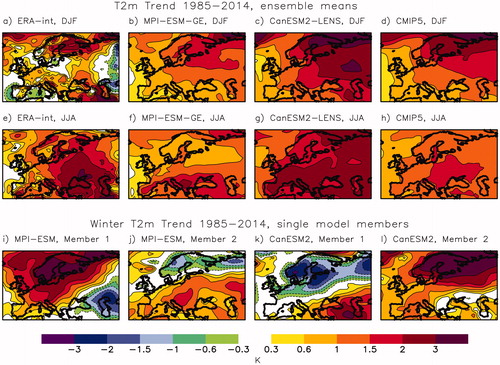
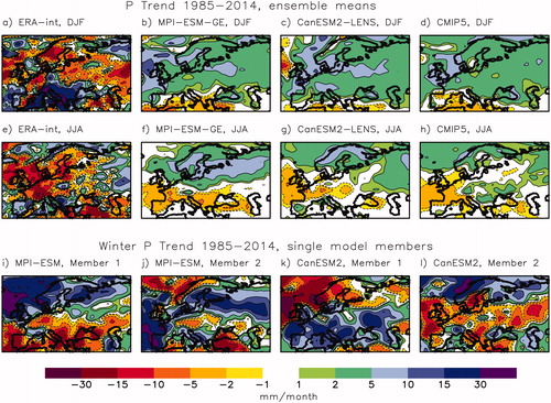
Fig. 2. As Fig. 1 but for precipitation. Shown are trends in mm/month per 30 years.

In summer, the ERA-interim trends were positive almost everywhere in Europe. Spatial variations were smaller than in winter. The strongest warming occurred around the Black Sea (up to 3 °C) while no warming is seen over the North Atlantic. The model ensemble means generally reproduce this observed pattern with larger warming trends in southeastern and southern Europe compared to western Europe and the Atlantic (Fig. 1d,f,h). The warming is largest in CanESM2-LENS. MPI-ESM-GE shows the smallest T2m increase over northern Europe among the model ensembles.

The winter P trend in ERA-interim (Fig. 2a) is very heterogeneous with a strong increase of P over the Mediterranean Sea (locally up to 30 mm/month between 1985 and 2014) and decreasing P from the Baltic Sea towards eastern Europe, over the Scandinavian mountain range and over the Nordic Seas. Similar as for winter T2m trends, large differences occur on small spatial scales. The model ensemble means show comparatively large small-scale variability in winter P trends as well (Fig. 2c,e,g), and the trend patterns over Europe differ strongly from the observed one. However, the models themselves generally agree on increased P in the northern and most of central European areas, and a decreasing trend over southern Europe in winter. As for temperature trends, the P-trend in single ensemble members is strongly varying and can differ completely from the ensemble means (Fig. 2i–k). The spatial variability is high on small scales in single members, which is similar to the observed trend pattern.

In summer, the observed P trends are dominated by decreased P over eastern and southwestern Europe and increased P over northwestern Europe. This pattern is at least partly reproduced by the model ensemble means although large differences occur locally. As for the temperature, the trend patterns in single model ensemble members deviate strongly from the ensemble mean patterns.

3.2. Uncertainties in near future temperature and precipitation trends

In this section, we analyse trends and their standard deviations in the near future period between years 2021 and 2050. The temperature trend patterns (Fig. 3) do not strongly differ from the trends in the recent past period 1985–2014. The warming is slightly reduced in the 2021–2050 period in MPI-ESM-GM and the RCP4.5 ensemble of CMIP5 over most of Europe, while in CanESM2-LENS and in CMIP5-RCP8.5 it is comparable to its recent past period. This is mainly due to reduced greenhouse gas emissions in the RCP4.5 scenario, used in MPI-ESM-GE and CMIP5-RCP4.5, compared to the RCP8.5 scenario, used in CanESM2-LENS and CMIP5-RCP8.5. However, in southern Europe, the warming in CanESM2-LENS is larger than in CMIP5-RCP8.5.

Fig. 3. Ensemble means of winter and summer two-meter air temperature trends (Kelvin per 30 years) in MPI-ESM-GE, CanESM2-LENS and CMIP5 (RCP4.5 and RCP8.5) between 2021 and 2050 (a–h) and their standard deviation across ensemble members (i–p). Note that the color-scale is not linear.

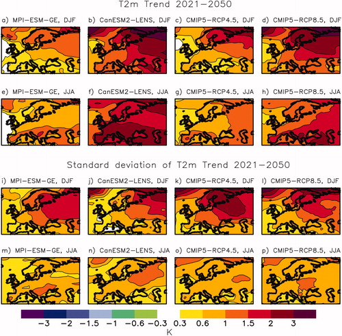
We find that one standard deviation of winter T2m trends in the model ensembles are of similar size as the 30-year trends themselves. All model ensembles show a decreasing standard deviation from northeast to southwest in Europe. Winter T2m trends in single simulations can differ up to around ±3 °C from the ensemble mean trend at the grid-point scale. Thus, winter temperature reductions until year 2050 are possible everywhere in Europe in CMIP5-RCP4.5 and MPI-ESM-GE (both using the RCP4.5 scenario), but also a temperature increase up to 4 °C can occur. These results are in agreement with Suárez-Gutiérrez et al. (2018) who showed large variations of European summer temperatures at 1.5 °C and 2 °C global warming levels in different ensemble members of the MPI-ESM-GE.

The large-scale patterns of precipitation trends until 2050 in the model ensemble means differ somewhat from those of 1985–2014 (compare Figs. 2 and 4). MPI-ESM-GE and CMIP5-RCP4.5 show a northward shift of the area with P-decrease both in summer and winter. Further, the summer P increase in northern Europe is smaller compared to 1985–2014. CanESM2-LENS shows also an increase of the area with negative P-trends until 2050 compared to the period 1985–2014. This can be seen in CMIP5-RCP8.5 as well, but less pronounced compared to CanESM2-LENS. Both MPI-ESM-GE and CanESM2-LENS show strongly increased winter P until 2050 in a region north of Scotland – west of Norway over the northeastern North Atlantic Ocean. The summer trend pattern of the four ensemble means agree relatively well with each other.

Fig. 4. As Fig. 3 but for precipitation.

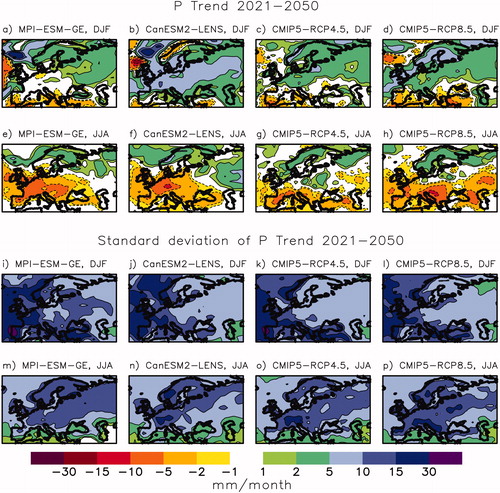
The spread of P-trends until 2050 is very high in both winter and summer (Fig. 4i-p). One standard deviation of P-trends is almost everywhere over Europe larger than the mean trend, indicating that the relative uncertainty in future P-trends is even larger than the one in T2m-trends. The uncertainties of P-trends in winter and summer agree well between the two large ensembles. The largest uncertainties in winter trends occur in western and southern Europe with standard deviations of the trends of up to 30 mm/month. One standard deviation of summer P-trends reaches about 10–20 mm/month in most regions and is relatively homogeneous distributed across Europe. In southern Europe, P-trends vary less but this goes along with much smaller precipitation totals in summer. Even in the regions with the largest trends, the internal variability is much larger than the trends themselves. Over northern Europe, one standard deviation of P-trend is around two to five times larger than the trend itself in both winter and summer; over southern Europe in summer, this factor is around one to two. Due to a somewhat stronger trend signal in CanESM2-LENS and CMIP5-RCP8.5, the signal to noise ration for the P-trend is somewhat larger than in MPI-ESM-GE and CMIP5-RCP8.5.

The multi-model ensembles of CMIP5 simulations indicate a very similar spread of temperature and precipitation trends across models as the single model ensembles from MPI-ESM and CanESM2. This clearly highlights the importance of internal variability for the total uncertainties in future climate trends since the CMIP5 ensembles include both uncertainties from internal variability and model uncertainties.

We also calculated the percentage of simulations with positive T2m and P-trends between 2021 and 2050 in MPI-ESM-GE and CanESM2-LENS over Europe. While CanESM2-LENS simulates a warming for almost all members over most of Europe in both winter and summer, the warming in MPI-ESM-GE is less robust across ensemble members; in winter, between 60% and 80% of the members simulate a warming, in summer between 75% and 95%. The robustness of the sign of P-trends until 2050 is much smaller than for temperature in most European regions in both ensembles.

3.3. Uncertainties in long-term future climate trends

The traditional perception for long term future climate trends is that the contribution of internal variability to the uncertainty is small compared to model errors and uncertainties due to emission scenarios. Hawkins and Sutton (2009) estimated that at 80-year lead times, internal variability contributes with 1–2% and around 10% to global and regional future temperature uncertainties, respectively. In this section, we analyse the uncertainties of regional future trends over Europe until year 2100 in the MPI-ESM-GE using the lower RCP4.5 emission scenario, the CanESM2-LENS using the high RCP8.5 emission scenario, and the CMIP5-ensembles under RCP4.5 and RCP8.5 conditions. We focus here only on the internal temperature variability and its potential importance for the long-term temperature trends in this section. For precipitation, the conclusions from section 3.2 are generally valid for the long-term trends as well; despite a growing change signal in P, the internal variability exceeds the P-trend almost everywhere in Europe.

Figure 5 shows trends and their variabilities in the four ensembles between years 2021 and 2100. As for the 30-year periods, we find a large-scale warming pattern with stronger warming in northern and northeastern Europe and somewhat smaller warming over western and southwestern Europe in winter. Winter T2m continues to increase everywhere after year 2050 (compare Fig. 3) and shows a positive trend between below 1 °C in southwestern Europe and about 3 °C in northeastern Europe until year 2100 in MPI-ESM-GE. In the CMIP5-RCP4.5 ensemble, the trend is about 0.5 °C higher than in the MPI-ESM-GE. CanESM2-LENS shows a T2m increase, which reaches between about 3 °C in southwestern Europe and almost 8 °C in the northeast. This agrees well with the ensemble mean of CMIP5-RCP8.5. However, summer warming is much larger in the CanESM2-LENS with more than 6 °C in most of Europe, except for in northern and northwestern Europe and over the ocean, compared to CMIP5-RCP8.5.

Fig. 5. As Fig. 3 but for the period 2021–2100. Shown are trends in Kelvin per 80 years.

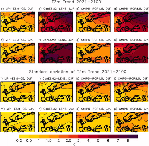
The spatial patterns of the spread of trends agree relatively well with the ones in the period 2021–2050. However, in the single model ensembles, MPI-ESM-GE and CanESM2-LENS, the spread is reduced compared to the 2021–2050 period. This is caused by the fact that many ensemble members show periods with opposing decadal to multi-decadal trends within the 80-year period until 2100. Long term variability in the North Atlantic, such as the Atlantic Meridional Overturning or the Atlantic Multi-decadal Oscillation, might affect the spread across model members and has time-scales of around 50–80 years. This variability might contribute to opposite trends at the 30-year scale while at 80-year periods a full cycle is included and opposite trends might cancel each other. However, one standard deviation of variability of temperature trends still reaches up to 1.5 °C in winter and up to 1 °C in summer. Thus, locally, internal variability can be of almost similar magnitude as the mean trend under the RCP4.5 scenario, and of similar magnitude as the difference between different emission scenarios. The uncertainty in trends in both CMIP5-ensembles is larger than in the single model ensembles because it includes both uncertainties due to internal variability and to model differences. The latter is growing the further we move into the future due to different climate sensitivities to the increasing forcing signal. In winter, the uncertainty is similar in CMIP5-RCP4.5 and CMIP5-RCP8.5 but in summer the spread is larger in CMIP5-RCP8.5.

A direct comparison to the results from Hawkins and Sutton (2009), who estimated that internal variability contributes with around 10% to the full uncertainty in regional future temperature scenarios until 2100, is difficult. However, a rough estimate, by dividing one standard deviation of trends in MPI-ESM-GE and CanESM2-LENS through the sum of one standard deviation of trends in the CMIP5-ensembles and the difference between ensemble mean trends in CMIP5-RCP8.5 and RCP4.5, provides that internal temperature variability contributes to around 15–20% to winter trends (2021–2100) in Northern Europe and 5–10% to summer trends. In southern Europe, this would be around 10–15% in winter and 5–10% in summer.

3.4. Case study southern Sweden

The summer 2018 and the winter 2019/2020 were the warmest in the observational time record in southern Sweden (SSWE) based on all station observations in southern Sweden performed by the Swedish Meteorological and Hydrological Institute (SMHI). Both records can likely be attributed to a combination of extreme, persisting weather conditions and an ongoing warming trend. The long-term temperature observations from Uppsala indicate high temperature variability in southern Sweden at interannual to multi-decadal time scales (Fig. 6). Two metre air temperature (T2m) trends in Uppsala in Sweden over consecutive 30-year periods between 1722 and 2017 varied strongly, and individual 30-year periods showed trends exceeding ±2 °C per 30 years. There is no clear difference in the spread of trends between the four seasons. Note that the external forcing between the various 30-year periods changed and that the number of periods is too small to estimate the entire range of possible 30-year trends from the observations.

Fig. 6. Distribution of observed seasonal temperature trends over 30-year periods in Uppsala between 1722 and 2017 (number of cases per 0.5 K interval).

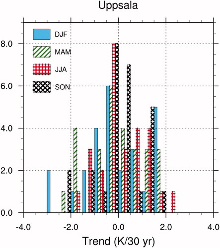
Here, we analyse more in detail the regional future trends of T2m and P, their spread and possible reasons for the spread in the SSWE region. We defined SSWE as the area 56°N − 60°N, 12°E − 17°E. The average temperature over SSWE in the ERA-interim reanalyses data is varying in line with observations from the weather station in Uppsala (r around 0.9 for all seasons in the ERA-interim period). This allows therefore for some comparison of variations and trends in the model results for southern Sweden to observations from Uppsala. The observational results showed that the trends over different historical 30-year periods vary for all seasons between roughly +2 °C and −2 °C or even more (Fig. 6). This spread agrees nicely with the simulated spread in our model ensembles in both the recent historical period (1985–2014, not shown) and the future period 2021–2050 in winter while the spread is smaller in the model ensembles compared to the observations in summer, particularly in CanESM2-LENS (Fig. 7).

Fig. 7. Probability distribution of two-meter air temperature (top) and precipitation (bottom) trends in southern Sweden in winter (left) and summer (right) between 2021 and 2050. Shown are trends per 30 years. Intervals for temperature are 0.5K, for precipitation 5mm/month.

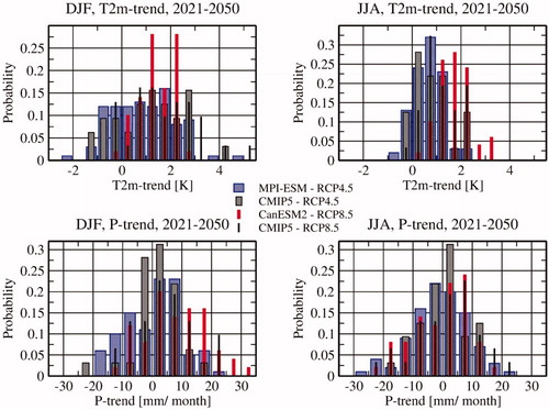
Figure 7 shows a similar probability distribution of 30-year T2m trends until year 2050 in both MPI-ESM-GE and in CMIP5-ensembles while CanESM2-LENS shows a smaller spread in winter. This difference can only partly be explained by the smaller number of members in CanESM2-LENS compared to MPI-ESM-GE; even 50 randomly selected members from MPI-ESM-GE show a larger spread of T2m trends than the 50 CanESM2-LENS members (not shown). Since we do not find a general difference in spread between CMIP5-RCP4.5 and CMIP5-RCP8.5, the smaller spread in CanESM2-LENS compared to MPI-ESM-GE can not be linked to the usage of a different scenario forcing.

For P, we see a slightly higher probability for both extremely positive and negative trends in MPI-ESM-GE than in the other model ensembles in summer. While the distribution for P and summer T2m trends show broad similarities with a Gaussian distribution, the distribution of winter T2m trends is more uniform with rather similar probabilities for trends between −1 °C and +3 °C. In addition to this uniform distribution, a few extreme ensemble members show much larger positive or negative wintertime trends reaching up to a warming of 5 °C or a cooling of more than −2 °C in MPI-ESM-GE.

Probability distributions of future trends of single variables are a helpful tool for risk management of climate change. However, combined changes of T2m and P are often of more relevance for adaptation. E.g., droughts would become much more severe if a decrease in P is accompanied by an increase of T2m. Although, it is not the aim of this study to analyse compound events and their risks in detail, we here analyse if trends in T2m and P in southern Sweden are connected to each other (Fig. 8). In winter, there is a tendency that ensemble members with stronger warming also have more positive P trends. However, the correlation between P and T2m trends is not very large (r = 0.33 and r = 0.34 in MPI-ESM-GE and CanESM2-LENS), although significant at the 95% significance level. In summer, we find the opposite response: stronger T2m trends are often related with a more negative trend in P (r = −0.41 and r = −0.44 in MPI-ESM-GE and CanESM2-LENS). These trends in T2m and P can be related to trends in the large scale atmospheric circulation as Fig. 9 reveals. Large winter warming trends in SSWE are connected to negative sea level pressure (SLP) trends over the Nordic Seas and positive SLP trends from the subtropical North Atlantic towards southeastern Europe. This leads to increased advection of warm and humid air from the southwest towards southern Sweden. At the same time, positive T2m trends from northwestern Europe across the entire of Asia occur. This extension of T2m-trends across Asia is more pronounced in MPI-ESM-GE than in CanESM2-LENS despite a stronger correlation with the SLP in CanESM2-LENS. In summer, in contrast, positive SLP-trends over Scandinavia lead to local drying and warming and to intensified advection of warmer and drier air from the east towards southern Scandinavia and to western Europe. Obviously, multi-decadal trends in the atmospheric circulation are the main driver for the simulated temperature trends in southern Sweden until 2050. Figure 9b and f indicate that trends in the North Atlantic Oscillation (NAO, defined as normalised SLP differences between Iceland and Azores in winter) can be one contributing driver for the winter T2m trends. Such a positive correlation between NAO and winter T2m in SSWE is revealed by Fig. 10a and e, as expected from previous studies (e.g. Jönsson and Bärring, 1994). The linkage of winter SSWE T2m trends to the NAO is more pronounced in CanESM2-LENS compared to MPI-ESM-GE.

Fig. 8. Scatterplot of precipitation and two-meter temperature trends in southern Sweden in winter (left) and summer (right) in the period 2021–2050 in the MPI-ESM-GE (a-b) and CanESM2-LENS (c-d). Shown are trends per 30 years.

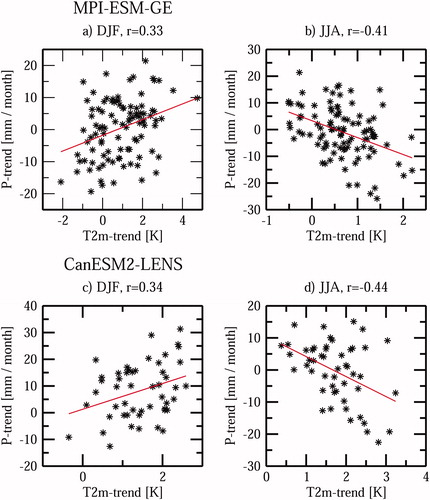
Fig. 9. Correlation between winter trends in T2m in southern Sweden in 2021–2050 and winter T2m trends in 2021–2050 (a and e), and winter sea level pressure (SLP) trends in 2021–2050 (b and f) in the MPI-ESM-GE (a–d) and CanESM2-LENS (e–h). (c, d, g and h) show the same as (a, b, e and f) but for summer T2m and SLP. Using a two-sided t-test, correlation coefficients above 0.2 and 0.29 are statistically significant at the 95% level assuming 100 degrees of freedom (MPI-ESM-GE,100 ensemble members) and 50 degrees of freedom (Can-ESM-LENS, 50 ensemble members), respectively.

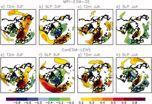
Fig. 10. Scatterplot of winter T2m-trends in southern Sweden in 2021–2050 in MPI-ESM-GE and CanESM2-LENS versus winter NAO-index trends (a and e), winter T2m-anomalies averaged over the first 5 years of the 2021–2050 year period (2021–2025, b and f), sea ice area trends in the Barents/Kara Seas in 2021-2050 (c and g), trends in the sea surface temperature (SST) of the subpolar gyre (SPG) in 2021–2050 (d and h).

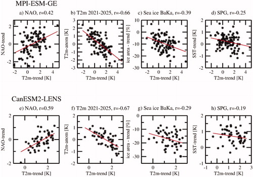
The spread of the simulated trends across model members might partly be explained by the fact that initial conditions between the model simulations differ strongly from each other. In reality, we know the initial state (with much smaller uncertainties). Thus, it is important to investigate if the knowledge of the initial state could reduce the spread of potential future trends. As expected, ensemble members with anomalously warm conditions in southern Sweden in the years 2021–2025 (warm compared to the ensemble mean T2m in 2021–2025) show withmuch higher probability a low or negative winter trend between 2021 and 2050 compared to members starting from anomalously cold conditions (Fig. 10b,f). For periods shorter than 5 years (e.g. only year 2021 or average of 2021–2022), the linkage to the trend of the entire 30-year period is small. Warm (cold) conditions in the first years could be part of multi-decadal variability, which is in its warm (cold) phase around 2021. In this case, one might assume that also the time period directly before 2021 can provide information on the trend in the 2021–2050 period. However, T2m in SSWE of the last five years (2016–2020) or of other time periods (1-year, 10-year means, seasonal means) before the start of the 2021–2050 period do not show any significant correlation with the winter T2m trend in 2021–2050 in neither MPI-ESM-GE nor CanESM2-LENS (not shown). We further test the relation between different other climate indices and T2m trends in SSWE in winter. Decadal to multi-decadal variability in the ocean and sea ice are potentially important for T2m trends at these time scales. However, correlations between different oceanic or sea ice indices and T2m trends in SSWE are not very high. The highest correlation that we found is between sea ice trends in the Barents/Kara Sea and SSWE T2m (r = −0.39 and r = −0.29 in MPI-ESM-GE and CanESM2-LENS Fig. 10c,g). This is in line with results from Koenigk et al. (2019) who showed that Barents/Kara Seas sea ice area is important for northern European winter T2m variability, mainly through thermodynamic effects.

The Atlantic Multi-decadal Oscillation is not significantly correlated with the T2m trend and the correlation between sub-polar gyre sea surface temperature (SST) trends and T2m in SSWE is also small, although significant at the 95% significance level in MPI-ESM-GE (Fig. 10d,h). These results indicate that the knowledge of initial conditions will only lead to a moderate reduction of the uncertainty in potential future temperature trends in SSWE.

4. Discussions and conclusions

In this study, we analysed large ensembles from two different global climate models and the CMIP5 multi-model ensemble, and investigated the uncertainty due to internal variability in multi-decadal temperature and precipitation trends over Sweden and Europe.

We find that internal variability leads to very large spread in temperature and precipitation trends in all seasons at 30-year time scales. Single ensemble members locally deviate up to about ±3 °C from the ensemble mean 30-year temperature trend. Thus, the variations are much larger than the mean warming trend itself until year 2050 under both RCP4.5 and RCP8.5 emission scenarios. These results agree qualitatively with previous studies that indicate large impact of the internal variability on local climate trends. Deser et al. (2014) found for North America standard deviations of 50-year winter temperature trends between 0.5 °C and 2 °C in winter and 0.5 °C and 1.25 °C in summer based on the 40-member ensemble of CCSM3. Similar to our results for Europe, the largest variability takes place in the north in the winter while more southern latitudes show a small annual cycle of trend variabilies. Bengtsson and Hodges (2019) analysed annual mean 50-year trends in the MPI-ESM-GE for the period 1850–2005 and found differences between minimum and maximum annual local temperature trends of up to 3 °C/50 years over northern Europe. Results from ensembles of CORDEX simulations and a single regional model downscaling over Europe for 2020–2049 (von Trentini et al., 2019) show a similar pattern of trend variability but generally lower standard deviations compared to MPI-ESM-GE and CanESM2-LENS. The CORDEX simulations show also lower variability of temperature trends compared to the CMIP5-ensemble. This is likely due to the fact that it is based on a smaller number of driving global models.

The uncertainty due to internal variability is even more pronounced for precipitation. Locally, the deviation from the mean trend can be several times larger than the mean trend itself. Even these results agree generally with previous studies (e.g. Deser et al., 2014; Bengtsson and Hodges, 2019). Comparing to results from Deser et al. (2014), the signal to noise ratio for precipitation seems to be smaller over Europe than over North America although time periods between our study and Deser et al. (2014) are of different length and thus not directly comparable.

Internal variability is not only important for uncertainties of trends on time-scales of 30 years but even for trends until year 2100 although the spread of T2m trends across ensemble members is reduced in both MPI-ESM-GE and CanESM2-LENS compared to the 2021–2050 period. This is due to the fact that multi-decadal variations with different sign often cancel each other at the 80-year scale while for 30-year periods they could either lead to additional or dampened warming. However, the impact of internal variability is still of the same size as the uncertainty between different emission scenarios (e.g. between RCP2.6 and RCP4.5 or RCP4.5 and RCP6.0) and extreme trends can even differ as much as the CMIP5 ensemble means of RCP4.5 and RCP8.5. Often, the signal to noise ratio is used as criteria for the importance of internal variability for future climate change. This covers the fact that internal variability still matters on longer time-scales; a relatively smaller variability compared to the signal does not necessarily mean for adaptation measures that the uncertainty due to variability is less important. Thus, internal variability must even be taken into account for future projections until 2100. This would be of particular importance in a world following the Paris agreement where the uncertainty from future emission pathways would be reduced.

Comparison between the spread of 30-year temperature trends in southern Sweden in the models and the estimated spread of 30-year temperature trends from the almost 300-year long observational record of Uppsala (Sweden, Moberg and Bergström, 1997) indicate that the spread of trends due to internal variability is rather realistically simulated by the models.

The uncertainties of trends in temperature and precipitation in southern Sweden due to internal variability are closely linked to trends in the large scale atmospheric circulation. This is in line with similar findings for other local areas (e.g. Deser et al., 2014; Horton et al., 2015; Koenigk et al., 2019). These circulation trends seem to be mainly due to intrinsic atmospheric variability. Further, our results show for the example of southern Sweden that knowledge of initial conditions seems to provide only limited prediction skill for T2m and P trends of the following 30 years.

The uncertainties in trends in the two large single model ensembles (MPI-ESM-GE, CanESM-LENS) are of similar magnitude as the spread in the 34 single CMIP5 models for 30-year periods. This indicates the importance of internal variability for the total uncertainty in future projections at these time scales. It also indicates that differences between CMIP-simulations with different models can be to an important part due to internal climate variability. For the longer period until 2100, the spread among single CMIP5 models is substantially larger due to different climate sensitivities in the various CMIP5 models. Comparing trends in the CMIP5-RCP4.5 with the CMIP5-RCP8.5 ensemble shows that parts of the larger trends in CanESM2-LENS compared to MPI-ESM-GE over Europe can be explained by the higher emission scenario. However, the somewhat different variability patterns in CanESM2-LENS compared to MPI-ESM-GE can not be explained by the usage of a different forcing scenario. Although the RCP4.5 and RCP8.5 ensembles of CMIP5 show some difference at the local scale, they do not show generally different trend variability patterns.

Generally, the results regarding the importance of internal variability for multi-decadal trends are robust across the model ensembles used in this study although locally the choice of the model plays a role. All ensembles highlight the relevance of internal variability for long-term future climate trends. These results agree well with findings by Deser et al. (2014) for North America and with the recent studies from Bengtsson and Hodges (2019) and Suárez-Gutiérrez et al. (2018).

Thus, uncertainties from internal variability must be taken into account for adaptation activities by stakeholders and decision-makers. Statements about future climate at the regional scale (e.g. southern Sweden) should consider the contribution from internal variability, especially for the near future (i.e. 20–50 years). On this temporal and spatial scale, the actual outcome of the future climate may well be different from the projected ensemble mean.

Acknowledgements

We thank the Max Planck Institute for Meteorology for producing and providing the data from the Max Planck Institute Grand Ensemble simulations. We thank the Canadian Centre for Climate Modelling and Analysis (CCCma) and the Canadian Sea Ice and Snow Evolution Network (CanSISE) Climate Change and Atmospheric Research (CCAR) Network project for producing and publishing the large ensemble simulation with CanESM2. We acknowledge the World Climate Research Programme’s Working Group on Coupled Modelling, which is responsible for CMIP, and we thank the modelling groups for producing and publishing their model output.

Disclosure statement

No potential conflict of interest was reported by the authors.

Additional information

Funding

This study has been made possible by support of the Rossby Centre at the Swedish Meteorological and Hydrologial Institute (SMHI) together with the Swedish Research Council FORMAS project REGTREND and the JPI-Climate-Belmont Forum project 407, InterDec. The research leading to these results have also received support from the German Federal Ministry of Education and Research (BMBF) through the CLIMPRE InterDec project (FKZ: 01LP1609A; ET, DM).

References

- Arora, V. K. 2003. Simulating energy and carbon fluxes over winter wheat using coupled land surface and terrestrial ecosystem models. Agric. For. Meteorol. 118, 21–47. doi:10.1016/S0168-1923(03)00073-X
- Arora, V. K., Scinocca, J. F., Boer, G. J., Christian, J. R., Denman, K. L. and co-authors. 2011. Carbon emission limits required to satisfy future representative concentration pathways of greenhouse gases. Geophys. Res. Lett. 38, 1–6. doi:10.1029/2010GL046270
- Bengtsson, L. and Hodges, K. I. 2019. Can an ensemble climate simulation be used to separate climate change signals from internal unforced variability? Clim. Dyn. 52, 3553–3573. doi:10.1007/s00382-018-4343-8
- Bittner, M., Schmidt, H., Timmreck, C. and Sienz, F. 2016. Using a large ensemble of simulations to assess the Northern Hemisphere stratospheric dynamical response to tropical volcanic eruptions and its uncertainty. Geophys. Res. Lett. 43, 9324–9332. doi:10.1002/2016GL070587
- Christian, J. R., Arora, V. K., Boer, G. J., Curry, C. L., Zahariev, K. and co-authors. 2010. The global carbon cycle in the CCCma earth system model CanESM1: preindustrial control simulation. J. Geophy. Res. 115, 1–20. doi:10.1029/2008JG000920
- Dai, A. and Bloecker, C. E. 2019. Impacts of internal variability on temperature and precipitation trends in large ensemble simulations by two climate models. Clim. Dyn. 52, 289–306. doi:10.1007/s00382-018-4132-4
- Dee, D. P., Uppala, S. M., Simmons, A. J., Berrisford, P., Poli, P. and co-authors. 2011. The ERA-Interim reanalysis: configuration and performance of the data assimilation system. Q. J. R. Meteorol. Soc. 137, 553–597. doi:10.1002/qj.828
- Deser, C., Knutti, R., Solomon, S. and Phillips, A. S. 2012. Communication of the role of natural variability in future North American climate. Nat. Clim. Change 2, 775–779. doi:10.1038/nclimate1562
- Deser, C., Phillips, A., Bourdette, V. and Teng, H. 2012. Uncertainty in climate change projections: the role of internal variability. Clim. Dyn. 38, 527–546. doi:10.1007/s00382-010-0977-x
- Deser, C., Phillips, A. S., Alexander, M. A. and Smoliak, B. V. 2014. Projecting North American climate over the next 50 years: uncertainty due to internal variability. J. Clim. 27, 2271–2296. doi:10.1175/JCLI-D-13-00451.1
- Fischer, E. M., Sedlacek, J., Hawkins, E. and Knutti, R. 2014. Models agree on forced response pattern of precipitation and temperature extremes. Geophys. Res. Lett. 41, 8554–8562. doi:10.1002/2014GL062018
- Giorgetta, M. A., Jungclaus, J., Reick, C. H., Legutke, S., Bader, J. and co-authors. 2013. Climate and carbon cycle changes from 1850 to 2100 in MPI‐ESM simulations for the Coupled Model Intercomparison Project phase 5. J. Adv. Model. Earth Syst. 5, 572–597. doi:10.1002/jame.20038
- Hawkins, E. 2011. Our evolving climate: communicating the effects of climate variability. Weather 66, 175–179. doi:10.1002/wea.761
- Hawkins, E. and Sutton, R. 2009. The potential to narrow uncertainties in regional climate predictions. Bull. Am. Meteor. Soc. 90, 1095–1107. doi:10.1175/2009BAMS2607.1
- Hawkins, E. and Sutton, R. 2012. Time of emergence of climate signals. Geophys. Res. Lett. 39, 1–6. doi:10.1029/2011GL050087
- Hedemann, C., Mauritsen, T., Jungclaus, J. and Marotzke, J. 2017. The subtle origins of surface-warming hiatuses. Nat. Clim. Change 7, 336–339. doi:10.1038/nclimate3274
- Horton, D. E., Johnson, N. C., Singh, D., Swain, D. L., Rajaratnam, B. and co-authors. 2015. Contribution of changes in atmospheric circulation patterns to extreme temperature trends. Nature 522, 465–469. doi:10.1038/nature14550
- Jahn, A., Kay, J. E., Holland, M. M. and Hall, D. M. 2016. How predictable is the timing of a summer ice-free Arctic? Geophys. Res. Lett. 43, 9113–9120. doi:10.1002/2016GL070067
- Jönsson, P. and Bärring, L. 1994. Zonal index variations, 1899–1992: links to air temperature in southern Scandinavia. Geogr. Ann. Ser. A Phys. Geogr. 76, 207–219.
- Jungclaus, J. H., Fischer, N., Haak, H., Lohmann, K., Marotzke, J. and co-authors. 2013. Characteristics of the ocean simulations in the Max Planck Institute Ocean Model (MPIOM) the ocean component of the MPI-Earth system model. J. Adv. Model. Earth Syst. 5, 422–446. doi:10.1002/jame.20023
- Kirchmeier-Young, M. C., Zwiers, F. W. and Gillett, N. P. 2017. Attribution of extreme events in Arctic sea ice extent. J. Clim. 30, 553–571. doi:10.1175/JCLI-D-16-0412.1
- Koenigk, T., Gao, Y., Gastineau, G., Keenlyside, N., Nakamura, T. and co-authors. 2019. Impact of Arctic sea ice variations on winter temperature anomalies in northern hemispheric land areas. Clim. Dyn. 52, 3111–3137. doi:10.1007/s00382-018-4305-1
- Knutti, R. and Sedlacek, J. 2013. Robustness and uncertainties in the new CMIP5 climate model projections. Nat. Clim. Change 3, 369–373. doi:10.1038/nclimate1716
- Maher, N., Milinski, S., Suarez‐Gutierrez, L., Botzet, M., Dobrynin, M. and co-authors. 2019. The Max Planck Institute Grand Ensemble: enabling the exploration of climate system variability. J. Adv. Model. Earth Syst. 11, 2050–2021. doi:10.1029/2019MS001639
- Marotzke, J. 2019. Quantifying the irreducible uncertainty in near-term climate projections. Wiley Interdiscip. Rev. Clim. Change 10, e563. doi:10.1002/wcc.563
- Moberg, A. and Bergström, H. 1997. Homogenization of Swedish temperature data. Part III: the long temperature records from Uppsala and Stockholm. Int. J. Climatol. 17, 667–699. doi:10.1002/(SICI)1097-0088(19970615)17:7<667::AID-JOC115>3.0.CO;2-J
- Moberg, A., Jones, P. D., Barriendos, M., Bergström, H., Camuffo, D. and co-authors. 2000. Day‐to‐day temperature variability trends in 160‐ to 275‐year‐long European instrumental records. J. Geophys. Res. 105, 22849–22868. doi:10.1029/2000JD900300
- Mori, M., Watanabe, M., Shiogama, H., Inoue, J. and Kimoto, M. 2014. Robust Arctic sea-ice influence on the frequent Eurasian cold winters in past decades. Nat. Geosci. 7, 869–873. doi:10.1038/ngeo2277
- Niederdrenk, A. L. and Notz, D. 2018. Arctic sea ice in a 1.5 °C warmer world. Geophys. Res. Lett. 45, 1963–1971. doi:10.1002/2017GL076159
- Notz, D., Haumann, F. A., Haak, H., Jungclaus, J. H. and Marotzke, J. 2013. Arctic sea-ice evolution as modeled by Max Planck Institute for Meteorology’s Earth system model. J. Adv. Modell. Earth Syst. 5, 1–22.
- Ogawa, F., Keenlyside, N., Gao, Y., Koenigk, T., Yang, S. and co-authors. 2018. Evaluating impacts of recent Arctic sea ice loss on the northern hemisphere winter climate change. Geophys. Res. Lett. 45, 3255–3263. doi:10.1002/2017GL076502
- Rondeau-Genesse, G. and Braun, M. 2019. Impact of internal variability on climate change for the upcoming decades: analysis of the CanESM2-LE and CESM-LE large ensembles. Clim. Change 156, 299–314. doi:10.1007/s10584-019-02550-2
- Sigmond, M. and Fyfe, J. 2016. Tropical Pacific impacts on cooling North American winters. Nat. Clim. Change 6, 970–974. doi:10.1038/nclimate3069
- Suárez-Gutiérrez, L., Chao, L., Müller, W. A. and Marotzke, J. 2018. Internal variability in European summer temperatures at 1.5 °C and 2 °C of global warming. Environ. Res. Lett. 13, 064026. doi:10.1088/1748-9326/aaba58
- Suárez-Gutiérrez, L., Li, C., Thorne, P. W. and Marotzke, J. 2017. Internal variability in simulated and observed tropical tropospheric temperature trends. Geophys. Res. Lett. 44, 5709–5719. doi:10.1002/2017GL073798
- Taylor, K. E., Stouffer, R. J. and Meehl, G. A. 2012. An overview of CMIP5 and the experiment design. Bull. Am. Meteor. Soc. 93, 485–498. doi:10.1175/BAMS-D-11-00094.1
- Vihma, T. 2014. Effects of Arctic sea ice decline on weather and climate: a review. Surv. Geophys. 35, 1175–1214. doi:10.1007/s10712-014-9284-0
- von Storch, H. and Zwiers, F. 1999. Statistical Analysis in Climate Research. Cambridge University Press, Cambridge.
- von Trentini, F., Leduc, M. and Ludwig, R. 2019. Assessing natural variability in RCM signals: comparison of a multi model EURO-CORDEX ensemble with a 50-member single model large ensemble. Clim. Dyn. 53, 1963–1979. doi:10.1007/s00382-019-04755-8