On the use of reduced grids in conjunction with the Equator-Pole grid system

Abstract

This is a continuation of a previous paper by Starius, where for the solution of the shallow water equations on the sphere, we consider Equator-Pole grid systems consisting of one latitude-longitude grid covering an annular band around the equator, and two orthogonal polar grids based on modified stereographic coordinates. Here, we generalise this by letting an equatorial band be covered with a reduced grid system, which can decrease the total number of grid points by at least 20%, with no substantial change in accuracy. Centred finite differences of high order are used for the spatial discretisation of the underlying differential equations and the explicit fourth order Runge-Kutta method for the integration in time. In the paper mentioned above, we demonstrate accuracy in the total mass, which is much higher than needed for NWP, for smooth solutions. Here we show that this holds also for non-smooth solutions, by considering the Cosine bell no. 1 and the mountain problem no. 5 in Williamson et al., the solutions of which have discontinuous second and first order derivatives, respectively.

Keywords:

• conservation
• Equator-Pole grid systems
• overset grids
• reduced grids
• shallow water equations on the sphere

Keywords:

• AMS Subject Classification: 35L45
• 65M06

1. Introduction

In this continuation paper to Starius (2018), referred to as (S-E-P) below, we consider numerical methods for the shallow water equations on the sphere, using the Equator-Pole (E-P) grid system. We make use of a reduced grid system for an annular band around the equator, which is divided into segments, each covered with a lat-lon net. As in (S-E-P) the equatorial grid is complemented by two orthogonal polar grids obtained by suitably modified stereographic coordinates. The whole grid system is optimised by minimising a global measure of uniformity, namely the maximum of all deviation factors on the sphere, where as in (S-E-P), the deviation factor for a net rectangle is the greatest ratio of its side-lengths.

The methods of this paper give an accuracy in the total mass, which is considerably higher than needed for NWP. This was already shown for the smooth Rossby-Haurwitz wave example for the method in (S-E-P). Here it is also verified, with and without reductions, for non-smooth solutions by considering the Cosine bell no. 1 and the mountain problem no. 5 in Williamson et al. (1992), the former with second order and the latter with first order discontinuous derivatives in their solutions. We have also integrated the mountain problem for a time period of 5 years, with maximal relative errors in the total mass of order ${10}^{-5}.$ For the total energy the corresponding quantities were of order ${10}^{-2}.$

If K denotes the number of segments on a hemisphere, then there are 2 K-1 segments on the whole sphere, since the two segments closest to the equator are merged together. We note that K = 1 is the case considered in (S-E-P). By reductions the uniformity is improved and the total number of grid points can be decreased by 20% or more, with no substantial change in accuracy. For high resolution also the computing time will be reduced by a similar percentage. High order one-dimensional centred interpolation formulas are used to connect the discretisations on adjacent segments. The kind of deviations from uniformity that arise by changing the number of grid points on parallels do not cause any problems, at least not for the methods described in this paper.

We now briefly comment on some other methods considered in the literature. Our main sources are the two overview papers Staniforth and Thuburn (2012) and Williamson (2007). There are many other grid techniques than ours for the sphere, among which the most popular are the cubed sphere, the icosahedral and the Yin-Yang grid systems. The paper (S-E-P) contains a more detailed overview than the one given below.

Cubed sphere grids (Sadourny, 1972) consist of quadrilaterals and have been used for finite volume methods in, e.g. (Putman and Lin, 2007; Ullrich et al., 2010), for discontinuous Galerkin methods in, e.g. (Nair et al., 2005; Bao et al., 2014) and for finite difference methods in, e.g. (Ronchi et al., 1996). Some drawbacks are lack of orthogonality and deviation from uniformity, particularly at the 8 corner-points of the cube, where angles up to ${120}^o$ instead of the ideal ${90}^o$ occur.

Icosahedral grids (Williamson, 1968) are generally triangular and have been used for finite volume methods in, e.g. (Pudykiewics, 2011; Chen et al., 2014) and for discontinuous Galerkin methods in, e.g. (Giraldo, 2006; Läuter et al., 2008). At the 12 corner-points of the icosahedron there are angles up to ${72}^o$ instead of the ideal ${60}^o.$

The more recently developed Yin-Yang grid, in Kageyama and Sato (2004), is an overset grid system consisting of two congruent orthogonal subgrids based on spherical coordinates and having maximal deviation factor $\sqrt{2}.$ This grid has been used by, e.g. Qaddouri and Lee (2011) and for a full 3d model by Allen and Zerroukat (2016). Both this grid system and ours use overset and orthogonal grids, which leads to an obvious similarity between the two techniques.

The great importance of the axis of the Earth for the dynamics of the weather is clear. However, the Yin-Yang grid does not have good rotational symmetry properties relative to this axis, not even near the poles, for details see, e.g. Section 1 in (S-E-P). At the end of Section 3.4, we compare the Yin-Yang grids and ours with respect to the total number of grid points, both with the same number on the equator.

The paper is organised as follows. In Section 2, we introduce the set of governing equations, some notation, and also some coordinate systems. This section is essentially a summary of Section 2 in (S-E-P).

Section 3 is devoted to reduced grid systems for annular bands around the equator. Two methods, I and II, to divide the band into segments and then to connect them by interpolation, are considered in Sections 3.1 and 3.2. Method I is quite general and easy to implement but requires more interpolation coefficients than method II. However, method II has limitations in its applicability, which is discussed in Section 3.2. In Section 3.3, two different measures of uniformity, used to generate suitable grid systems for the sphere, are compared. In Section 3.4, an E-P grid system is constructed with square net rectangles at mid-latitudes, which is often required for NWP models.

In Section 4, we investigate our E-P grid systems numerically, both with and without reductions. Centred finite differences of high order are used for the spatial discretisations and the explicit fourth order Runge-Kutta method for the time integration. First some notation for various errors is introduced and then, in Section 4.1, smoothing by addition of a ’hyper-diffusion’ term is considered. For a discretisation method of order 2p a smoothing term of the same order is used, in contrast to the method in (S-E-P) where the order is always equal to 4. In Section 4.2, the rotation of the Cosine bell is considered and for this scalar advection example both the total mass and energy are obtained with much higher accuracy than for the height of the fluid. In Section 4.3, our results for an example by Läuter et al. (2005) show that the reduction techniques work quite well, the accuracy is very much the same for K = 1,2,3,4, particularly for the 6th order method. In Section 4.4, we consider zonal flow over an isolated mountain, example no. 5 in Williamson et al. (1992), with non-smooth solutions. The errors in the total mass shown in Table 6 are clearly small enough for NWP. We mention that no ‘corrections’ or ’fixers’ of any kind have been used.

In (S-E-P) further numerical examples are given, and also investigations of grid imprinting and comparisons between formal and computational orders of discretisation errors are considered.

2. Coordinate systems and governing differential equations

In this section, we introduce some notation and give a frame of reference for the paper. It is essentially a summary of Section 2 in (S-E-P).

2.1. Spherical coordinates and the shallow water equations

The transformation between Cartesian and spherical coordinates on the sphere is (1) $$\{\begin{array}{c}x=a\hspace{0.17em}\text{cos}\hspace{0.17em}\theta \hspace{0.17em}\text{cos}\hspace{0.17em}\lambda ,\hfill \\ y=a\hspace{0.17em}\text{cos}\hspace{0.17em}\theta \hspace{0.17em}\text{sin}\hspace{0.17em}\lambda , 0\le \lambda <2\pi , -\frac{\pi }{2}\le \theta \le \frac{\pi }{2},\hfill \\ z=a\hspace{0.17em}\text{sin}\hspace{0.17em}\theta ,\hfill \end{array}\mathrm{ }$$(1) where a is the radius of the sphere, λ the longitude, and θ the latitude. The advective form of the shallow water equations in spherical coordinates is given by (2) $$\begin{array}{c}{u}_t=-{(a\hspace{0.17em}\text{cos}\hspace{0.17em}\theta )}^{-1}(u{u}_{\lambda }+{\Psi }_{\lambda })-a^{-1}v{u}_{\theta }+(f+a^{-1}u\hspace{0.17em}\text{tan}\hspace{0.17em}\theta )v,\\ v_t=-{(a\hspace{0.17em}\text{cos}\hspace{0.17em}\theta )}^{-1}u{v}_{\lambda }-a^{-1}(v{v}_{\theta }+{\Psi }_{\theta })-(f+a^{-1}u\hspace{0.17em}\text{tan}\hspace{0.17em}\theta )u,\\ {\Psi }_t=-{(a\hspace{0.17em}\text{cos}\hspace{0.17em}\theta )}^{-1}(u_{\lambda }\Psi +u{\Psi }_{\lambda })-a^{-1}{(v\Psi )}_{\theta }+a^{-1}v\Psi \hspace{0.17em}\text{tan}\hspace{0.17em}\theta ,\end{array}$$(2) where $\Psi$ is the geopotential, $f=2\Omega \hspace{0.17em}\text{sin}\hspace{0.17em}\theta$ the Coriolis parameter, Ω the rotation rate of the sphere, and u and v the eastward and northward velocity components, respectively.

2.2. Standard and modified stereographic coordinates

Consider first the standard stereographic coordinates. The relation between these and spherical coordinates can be expressed as (3) $$\{\begin{array}{c}{x}_{st}=a q(\theta )\hspace{0.17em}\text{cos}\hspace{0.17em}\lambda ,\hfill \\ y_{st}=a q(\theta )\hspace{0.17em}\text{sin}\hspace{0.17em}\lambda ,\hfill \end{array}$$(3) where $q(\theta )=2\hspace{0.17em}\text{tan}\hspace{0.17em}(\phi /2),$ with the colatitude $\phi$ equal to $\frac{1}{2}\pi -\theta$ and $\frac{1}{2}\pi +\theta ,$ on the northern and southern hemisphere, respectively. We also need the map factor $m_f(\theta )=2/(1+\alpha \hspace{0.17em}\text{sin}\hspace{0.17em}\theta ),$ where α = 1 on the northern and −1 on the southern hemisphere.

Since the velocities in spherical coordinates, $u=a \hspace{0.17em}\text{cos}\hspace{0.17em}\theta d\lambda /dt,$ $v=a d\theta /dt,$ are not uniquely defined at the poles, we use instead the stereographic velocities $U=-d{x}_{st}/dt,V=d{y}_{st}/dt.$ Observe the use of the minus sign in the definition of U, intended to get nicer formulas, namely (4) $$\left(\begin{array}{c}u\\ v\end{array}\right)=A\left(\begin{array}{c}U\\ V\end{array}\right) \text{and} \left(\begin{array}{c}u\\ -v\end{array}\right)=A\left(\begin{array}{c}U\\ V\end{array}\right),\text{where}A=\left(\begin{array}{cc}\hspace{0.17em}\text{sin}\hspace{0.17em}\lambda & \hspace{0.17em}\text{cos}\hspace{0.17em}\lambda \\ \hspace{0.17em}\text{cos}\hspace{0.17em}\lambda & -\hspace{0.17em}\text{sin}\hspace{0.17em}\lambda \end{array}\right),$$(4) on the northern and southern polar regions, respectively. In (4(4) $$\left(\begin{array}{c}u\\ v\end{array}\right)=A\left(\begin{array}{c}U\\ V\end{array}\right) \text{and} \left(\begin{array}{c}u\\ -v\end{array}\right)=A\left(\begin{array}{c}U\\ V\end{array}\right),\text{where}A=\left(\begin{array}{cc}\hspace{0.17em}\text{sin}\hspace{0.17em}\lambda & \hspace{0.17em}\text{cos}\hspace{0.17em}\lambda \\ \hspace{0.17em}\text{cos}\hspace{0.17em}\lambda & -\hspace{0.17em}\text{sin}\hspace{0.17em}\lambda \end{array}\right),$$(4) ), U and V have been scaled by the factor $1/m_f(\theta ).$ The mapping (4(4) $$\left(\begin{array}{c}u\\ v\end{array}\right)=A\left(\begin{array}{c}U\\ V\end{array}\right) \text{and} \left(\begin{array}{c}u\\ -v\end{array}\right)=A\left(\begin{array}{c}U\\ V\end{array}\right),\text{where}A=\left(\begin{array}{cc}\hspace{0.17em}\text{sin}\hspace{0.17em}\lambda & \hspace{0.17em}\text{cos}\hspace{0.17em}\lambda \\ \hspace{0.17em}\text{cos}\hspace{0.17em}\lambda & -\hspace{0.17em}\text{sin}\hspace{0.17em}\lambda \end{array}\right),$$(4) ) is also used in Starius (2014), where it is derived by orthogonal projection of the vector (u, v) onto the equatorial plane.

Stereographic projection is only suitable for grid generation close to the poles. Here we will use a modification of (3(3) $$\{\begin{array}{c}{x}_{st}=a q(\theta )\hspace{0.17em}\text{cos}\hspace{0.17em}\lambda ,\hfill \\ y_{st}=a q(\theta )\hspace{0.17em}\text{sin}\hspace{0.17em}\lambda ,\hfill \end{array}$$(3) ), already recommended in Section 2.3 of (S-E-P), so that the lat-lon and our new modified stereographic grid points will coincide on the meridian corresponding to λ = 0, and automatically also on the meridians $\lambda =\frac{1}{2}\pi ,\pi ,\frac{3}{2}\pi ,$ provided the number of grid points on parallels in the last segment of the reduced grid is divisible by 4. The assumption for λ = 0 leads to new coordinates $(x\prime ,y\prime )$ related to $(x_{st},y_{st})$ by (5) $$\{\begin{array}{c}{x}_{st}=2a \hspace{0.17em}\text{tan}\hspace{0.17em}(x\prime /2),\hfill \\ y_{st}=2a \hspace{0.17em}\text{tan}\hspace{0.17em}(y\prime /2).\hfill \end{array}\mathrm{ }$$(5)

The modified coordinates $(x\prime ,y\prime )$ give rise to more uniform polar grids and will also simplify the connection between these grids and the last segments of the equatorial grid system. The shallow water equations expressed in the coordinates defined by (3(3) $$\{\begin{array}{c}{x}_{st}=a q(\theta )\hspace{0.17em}\text{cos}\hspace{0.17em}\lambda ,\hfill \\ y_{st}=a q(\theta )\hspace{0.17em}\text{sin}\hspace{0.17em}\lambda ,\hfill \end{array}$$(3) ) and (5(5) $$\{\begin{array}{c}{x}_{st}=2a \hspace{0.17em}\text{tan}\hspace{0.17em}(x\prime /2),\hfill \\ y_{st}=2a \hspace{0.17em}\text{tan}\hspace{0.17em}(y\prime /2).\hfill \end{array}\mathrm{ }$$(5) ), and the stereographic velocities U and V given in (4(4) $$\left(\begin{array}{c}u\\ v\end{array}\right)=A\left(\begin{array}{c}U\\ V\end{array}\right) \text{and} \left(\begin{array}{c}u\\ -v\end{array}\right)=A\left(\begin{array}{c}U\\ V\end{array}\right),\text{where}A=\left(\begin{array}{cc}\hspace{0.17em}\text{sin}\hspace{0.17em}\lambda & \hspace{0.17em}\text{cos}\hspace{0.17em}\lambda \\ \hspace{0.17em}\text{cos}\hspace{0.17em}\lambda & -\hspace{0.17em}\text{sin}\hspace{0.17em}\lambda \end{array}\right),$$(4) ), are written down in full detail in Section 2.3 of (S-E-P).

3. Reduced latitude-longitude grid systems covering an equatorial band

In this Section, we consider the possibility to utilise a reduced grid system for an annular band around the equator, cf. Gates and Riegel (1963), Kurihara (1965), Tolstykh and Shashkin (2012), and Starius (2014). We also mention the reduced Gaussian grids for spectral models in Hortal and Simmons (1991), reported to decrease the computing time by about 20%, and used by ECMWF in their operational model. Further, the papers Layton (2002) and Li (2018) are worth mentioning in this context. The band is divided into segments, each covered with a lat-lon net. Let n be the given number of grid points on the equator and K the number of segments on a hemisphere. Here we choose to have invariance under reflection in the equator, where the closest two segments are merged together, which implies that the total number of segments is 2 K-1 and the total number of subgrids is 2 K + 1. We recall that K = 1 is the case studied in (S-E-P).

We will later define latitudes ${\theta }_1<{\theta }_2<\dots <{\theta }_K$ such that the i:th segment S_i is bounded by ${\theta }_{i-1}$ and θ_i, $i=1,2,\dots ,K,$ where ${\theta }_0=0.$ Also the number of grid points n_i on a parallel in S_i has to be defined and satisfy $n_1>n_2>\dots >n_K,$ and the longitudinal steps are defined by $\Delta {\lambda }_i=2\pi /n_i,$ where $i=1,2,\dots ,K.$ We note that $n_1=n$ and when only one longitudinal step is used, for example for K = 1, it is called $\Delta \lambda .$

We now discretise the segments introduced above. Assume that all the latitudes θ_i are multiples of a latitudinal step $\Delta \theta .$ Consider for each i, with $1\le i\le K,$ the parallels ${\theta }_{i-1}+k\Delta \theta ,k=0,\dots ,s_i,$ where $s_i=({\theta }_i-{\theta }_{i-1})/\Delta \theta ,$ and let $S_i^d$ be the corresponding lat-lon net. Note that we have let $S_i^d$ and $S_{i+1}^d$ both contain the parallel corresponding to θ_i, which will ease the presentation in Sections 3.1 and 3.2. 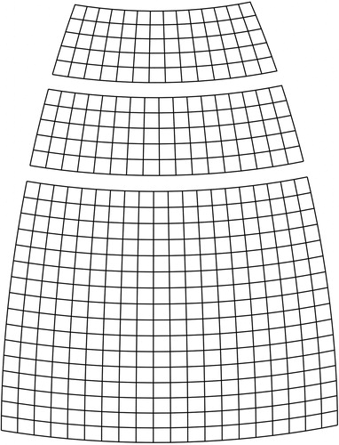When the discrete segments have been defined, we omit the parallel θ_i from $S_{i+1}^d,$ i = 1,…K-1, cf. Fig. 1.

Fig. 1. A small part $0\le \lambda \le {45}^o$ and $\theta \ge 0$ of a reduced grid for n = 160 and K = 3.

In this section, we will often use the fact that for a parallel with latitude θ and angular longitudinal step $\Delta \lambda ,$ the distance along the parallel between two consecutive grid points is $\Delta \lambda \hspace{0.17em}\text{cos}\hspace{0.17em}\theta .$

3.1. Method I: reduced latitude-longitude grid system

Here the number of segments K will be given by the user. The deviation factor at the equator is ${\sigma }_K=\Delta {\lambda }_1/\Delta \theta ,$ where $\Delta \theta$ will be the same for all discretised segments and determined later. We consider the segment $S_i^d$ and require that the distances between grid points on the parallel ${\theta }_{i-1}$ are equal to $\Delta {\lambda }_1,$ that is $\Delta {\lambda }_i\hspace{0.17em}\text{cos}\hspace{0.17em}{\theta }_{i-1}=\Delta {\lambda }_1,$ where $i=2,\dots ,K.$ Further, the maximal deviation factor for the segment $S_i^d$ is $\max (\Delta {\lambda }_i\hspace{0.17em}\text{cos}\hspace{0.17em}{\theta }_{i-1}/\Delta \theta , \Delta \theta /(\Delta {\lambda }_i\hspace{0.17em}\text{cos}\hspace{0.17em}{\theta }_i) ),$ which is obviously minimised, with respect to $\Delta {\lambda }_i/\Delta \theta ,$ when the two deviation factors in the $\max$ above are equal. We now have the equalities (6) $$\Delta {\lambda }_i\hspace{0.17em}\text{cos}\hspace{0.17em}{\theta }_{i-1}=\Delta {\lambda }_1 \text{and} \frac{\Delta {\lambda }_i\hspace{0.17em}\text{cos}\hspace{0.17em}{\theta }_{i-1}}{\Delta \theta }=\frac{\Delta \theta }{\Delta {\lambda }_i\hspace{0.17em}\text{cos}\hspace{0.17em}{\theta }_i},$$(6) and substituting $\Delta {\lambda }_i$ in the second equality by $\Delta {\lambda }_1/\hspace{0.17em}\text{cos}\hspace{0.17em}{\theta }_{i-1}$ and using ${\sigma }_K=\Delta {\lambda }_1/\Delta \theta ,$ gives (7) $$\frac{\hspace{0.17em}\text{cos}\hspace{0.17em}{\theta }_{i-1}}{\hspace{0.17em}\text{cos}\hspace{0.17em}{\theta }_i}={\sigma }_K^2,i=1,2,\dots ,K\Rightarrow \frac{1}{\hspace{0.17em}\text{cos}\hspace{0.17em}{\theta }_K}={\sigma }_K^{2K}.$$(7)

The transition from $S_K^d$ to a polar grid gives that ${\sigma }_K=m_f({\theta }_K)=2/(1+\hspace{0.17em}\text{sin}\hspace{0.17em}{\theta }_K),$ where $m_f(\theta )$ is the mapfactor in Section 2.2, cf. (12(12) $$\text{cos}\hspace{0.17em}{\overline{\theta }}_{i_0-1}\hspace{0.17em}\text{cos}\hspace{0.17em}{\overline{\theta }}_{i_0}=1/2.$$(12) ) in Section 3.2 of (S-E-P). This equality and the right hand side of (7(7) $$\frac{\hspace{0.17em}\text{cos}\hspace{0.17em}{\theta }_{i-1}}{\hspace{0.17em}\text{cos}\hspace{0.17em}{\theta }_i}={\sigma }_K^2,i=1,2,\dots ,K\Rightarrow \frac{1}{\hspace{0.17em}\text{cos}\hspace{0.17em}{\theta }_K}={\sigma }_K^{2K}.$$(7) ) imply (8) $$\text{cos}\hspace{0.17em}{\theta }_K={\left(\frac{1+\hspace{0.17em}\text{sin}\hspace{0.17em}{\theta }_K}{2}\right)}^{2K},$$(8) which can be solved by, e.g. Newton’s method. We then determine ${\sigma }_K=2/(1+\hspace{0.17em}\text{sin}\hspace{0.17em}{\theta }_K)$ and by using $\text{cos}\hspace{0.17em}{\theta }_i=\hspace{0.17em}\text{cos}\hspace{0.17em}{\theta }_{i-1}/{\sigma }_K^2={\sigma }_K^{-2i}$ we find θ_i, $i=1,2,\dots ,K$−1. Note that (8(8) $$\text{cos}\hspace{0.17em}{\theta }_K={\left(\frac{1+\hspace{0.17em}\text{sin}\hspace{0.17em}{\theta }_K}{2}\right)}^{2K},$$(8) ) implies that ${\theta }_K\to \frac{1}{2}\pi ,$ and hence ${\sigma }_K\to 1,$ as $K\to \infty .$

Now $\Delta \theta =\Delta {\lambda }_1/{\sigma }_K$ can be evaluated and for practical reasons modified by defining the integer m to be $\frac{1}{2}\pi /(\Delta {\lambda }_1/{\sigma }_K)$ rounded to the nearest integer and then redefining $\Delta \theta =\frac{1}{2}\pi /m.$ With $\Delta \theta$ known we now round the latitudes θ_i, $i=1,2,\dots ,K,$ to their closest multiples of $\Delta \theta .$ Finally we set $n_i=n\hspace{0.17em}\text{cos}\hspace{0.17em}{\theta }_{i-1},$ round it to the nearest integer, and define $\Delta {\lambda }_i=2\pi /n_i,i=2,\dots ,K.$

In Table 1, the overlap between the last segment in the reduced grid and the polar grid is 3, which only affects the number of parallels in this segment. An increase in the number of segments leads to a decrease in the total number of discretisation points and in the maximal deviation factor. In Fig. 1, a reduced grid with n = 160 and K = 3 is illustrated. More realistic resolutions for NWP are for instance n = 1000, K = 10, which gives p = 20.7% and $s_{10}=9,$ and n = 2000, K = 10, which gives p = 20.8% and $s_{10}=16.$ We recall that the above procedure requires only one-dimensional interpolation and that the coefficients in the formulas should be computed and stored during preprocessing. The number of sequences of interpolation coefficients is $n_1+2(n_2+\dots +n_{K-1})+n_K,$ which for high resolution is negligible compared to other storage requirements. A less general method using considerably fewer interpolation formulas is briefly described in Section 3.2.

Table 1. Reduced lat-lon grids with n = 360 and K segments on a hemisphere, using method I. Let N_K be the total number of discretisation points for given K, p_K is the decrease in per cent of N₁, that is $N_K=(1-p_K/100)N_1,$ and the quantity s_i is the number of parallels in the segment $S_i^d.$ The area of the polar regions as per cent of the total area of the sphere is given by $q_K=100(1-\hspace{0.17em}\text{sin}\hspace{0.17em}{\theta }_K).$

K	θ1	θ2	θ3	${\theta }_{K-1}$	θK	s1	s2	s3	$s_{K-1}$	sK	σK	pK	qK
1	45.0					56					1.1892	0	29
2	37.4	50.8				43	17				1.1269	9.5	23
3	34.0	46.8	55.1			38	14	11			1.0988	14.2	18
4	31.5	43.6	52.0		57.5	35	13	9		8	1.0848	16.2	16
5	29.1	40.3	48.8	55.3	60.0	32	12	9	7	7	1.0718	17.9	13
6	27.5	38.8	46.4	57.8	61.6	30	12	8	6	6	1.0641	19.4	12

A way to avoid scalability problems for the couplings between the reduced grid and the northern polar grid, say, is to let the former reach a high latitude. Since θ_K increases slowly with K (for instance K = 10 gives only ${\theta }_{10}={65.8}^o$) we will now consider a modification of method I, which is suitable for high latitudes. We choose K and determine the first K segments and the corresponding maximal deviation factor σ_K, and then complement this by the desired number of additional segments, each optimised with respect to σ_K. More specifically, additional latitudes ${\theta }_{K+1},{\theta }_{K+2},\dots$ can be determined by the equation $\text{cos}\hspace{0.17em}{\theta }_i={\sigma }_K^{-2i},i>K,$ and then also $n_i=n\hspace{0.17em}\text{cos}\hspace{0.17em}{\theta }_{i-1} \text{and} \Delta {\lambda }_i=2\pi /n_i,i>K,$ where the n_i have been rounded in a suitable way.

We conclude this subsection with two examples. For initial K = 3, we have ${\sigma }_3=1.0988$ and the corresponding latitudes are: 34.0, 46.8, 55.1, 61.9268, 67.0595, 71.1657, 74.4912, 77.2050, 79.4305, 81.2615. If we want the reduced grid to reach the polar circles, then we add two segments, so that K = 5, and reach latitude ${67}^o.$ The maximal deviation factor for the whole reduced grid system is still σ₃. In a second example, with initial K = 1 and ${\sigma }_1=1.1892,$ two segments have to be added, so that K = 3, for the reduced grid to pass the polar circles. There is obviously a trade-off between uniformity and the possibility to use a small number of segments.

3.2. Method II: reduced latitude-longitude grid system

This method is essentially applicable with a small number of segments and special choices of n. However, its range of applicability can be extended in ways described below. The notation and assumptions of Section 3.1 will be used here, and only a brief outline of the method will be given.

The method is based on the following simple idea. In a consecutive manner we replace q longitudinal mesh intervals in segment $S_i^d$ with q−1 intervals in the following segment $S_{i+1}^d.$ As for method I we require that $\Delta {\lambda }_i\hspace{0.17em}\text{cos}\hspace{0.17em}{\theta }_{i-1}=\Delta {\lambda }_1,$ where $i=2,\dots ,K,$ and further that each n_i, with i < K, is divisible by q. This implies that $\Delta {\lambda }_{i+1}/\Delta {\lambda }_i=n_i/n_{i+1}=q/(q-1).$ Further, $\Delta {\lambda }_i\hspace{0.17em}\text{cos}\hspace{0.17em}{\theta }_{i-1}=\Delta {\lambda }_{i+1}\hspace{0.17em}\text{cos}\hspace{0.17em}{\theta }_i$ together with (7(7) $$\frac{\hspace{0.17em}\text{cos}\hspace{0.17em}{\theta }_{i-1}}{\hspace{0.17em}\text{cos}\hspace{0.17em}{\theta }_i}={\sigma }_K^2,i=1,2,\dots ,K\Rightarrow \frac{1}{\hspace{0.17em}\text{cos}\hspace{0.17em}{\theta }_K}={\sigma }_K^{2K}.$$(7) ) leads to $\Delta {\lambda }_{i+1}/\Delta {\lambda }_i=\hspace{0.17em}\text{cos}\hspace{0.17em}{\theta }_{i-1}/\hspace{0.17em}\text{cos}\hspace{0.17em}{\theta }_i={\sigma }^2,$ where we write σ instead of σ_K, since σ is now independent of K. We choose q and determine σ and ${\vartheta }_0,$ where ${\vartheta }_0$ is the width of the reduced grid, by using $${\sigma }^2=\frac{q}{q-1} \text{and} \frac{2}{1+\hspace{0.17em}\text{sin}\hspace{0.17em}{\vartheta }_0}=\sigma .$$

We now determine θ_i by $\text{cos}\hspace{0.17em}{\theta }_i={\sigma }^{-2i},i=1,2,\dots$ until ${\theta }_i>{\vartheta }_0.$ Further, we can choose K from $|{\theta }_K-{\vartheta }_0|={\min }_i|{\theta }_i-{\vartheta }_0|$ and then redefine ${\vartheta }_0={\theta }_K.$ For low resolution it might be necessary to replace K by a smaller value in order to get a reasonable number of parallels in the segment $S_K^d.$ Since $n_1=n$ is known we can use $n_{i+1}=(q-1)n_i/q,\text{where}i=1,\dots ,K$-1, and then define $\Delta {\lambda }_i=2\pi /n_i,i=2,\dots ,K.$

The above works only if n is divisible by $q^{K-1},$ where K has our desired value, in which case the number of sequences of interpolation coefficients required is only q−1, provided symmetry is used to reduce the number of sequences whenever possible.

If we get a number $n_{i_0},$ with $i_0<K,$ not divisible by q, then $\lambda =2\pi$ will not correspond to grid points in $S_{i_0+1}^d.$ Since we now cannot have equidistant grid points in all our discretisations, we switch to a modification of method II, which allows that. From segment $S_{i_0+1}^d$ onward, we define $n_{i+1}=(q-1)n_i/q,$ for $i=i_0,\dots ,K$ and then round them to integers and define $\Delta {\lambda }_{i+1}=2\pi /n_{i+1},$ for $i=i_0,\dots ,K.$ This transition to method I is very simple but requires more sequences of interpolation coefficients.

For high resolution, we indicate an improvement of the above modification of method II. If $n_{i_0+1}$ is rounded to an integer divisible by q, then the interpolation between $S_{i_0+1}^d$ and $S_{i_0+2}^d$ can be done with the q−1 interpolation formulas. We still use method I for the interpolation between $S_{i_0}^d$ and $S_{i_0+1}^d.$ This can be repeated by choosing $n_{i_0+3}$ divisible by q, using method I between $S_{i_0+2}^d$ and $S_{i_0+3}^d,$ and then the q−1 interpolation formulas between $S_{i_0+3}^d$ and $S_{i_0+4}^d,$ etc.

We conclude this subsection by considering an example with q = 6, which preliminarily gives $\sigma =\sqrt{6/5}=1.0954.$ We have ${\vartheta }_0=55.7$ and the following sequence of latitudes determining the segments: 33.6, 46.0, 54.6, 61.2, 66.3, 70.4, 73.8, 76.6, 78.8, 80.7. Thus according to the above we choose K = 3, redefine ${\vartheta }_0={\theta }_3,$ and obtain a new $\sigma =2/(1+\hspace{0.17em}\text{sin}\hspace{0.17em}{\theta }_3)=1.1019.$ If n is divisible by 6², then method II works perfectly well for K = 3. However, if we want K > 3 and n is not divisible by 6³, we can use a modification as described above for the segments following $S_3^d.$

3.3. Comparison between two measures of uniformity

The measure of uniformity most commonly referred to in the literature is the ratio of maximum to minimum grid length, which we call γ in this section. Our main interest here is to investigate which measure of uniformity is best suited for grid generation. Our maximal deviation factor has already been used for this purpose, and we therefore now turn our focus to the ratio γ by studying two examples.

Example (i): Let S^d be a segment on the northern hemisphere bounded by the latitudes ${\theta }_1<{\theta }_2$ and consisting of a lat-lon net with the longitudinal step $\Delta \lambda .$ We define σ as the deviation factor for net rectangles at θ₁, that is $\sigma =\Delta \lambda \hspace{0.17em}\text{cos}\hspace{0.17em}{\theta }_1/\Delta \theta ,$ where $\Delta \theta$ is the latitudinal step, not yet determined. The ratio of maximum to minimum grid length on S^d is $$\gamma =\gamma (\sigma )=\frac{\Delta \lambda \hspace{0.17em}\text{cos}\hspace{0.17em}{\theta }_1}{\min ( \Delta \theta ,\Delta \lambda \hspace{0.17em}\text{cos}\hspace{0.17em}{\theta }_2 )}=\frac{\sigma }{\min (1,\sigma \hspace{0.17em}\text{cos}\hspace{0.17em}{\theta }_2/\hspace{0.17em}\text{cos}\hspace{0.17em}{\theta }_1 )},$$ from which it follows $$\gamma =\mathrm{ }\{\begin{array}{cc}\hspace{0.17em}\text{cos}\hspace{0.17em}{\theta }_1/\hspace{0.17em}\text{cos}\hspace{0.17em}{\theta }_2,\hfill & \sigma \le \hspace{0.17em}\text{cos}\hspace{0.17em}{\theta }_1/\hspace{0.17em}\text{cos}\hspace{0.17em}{\theta }_2,\hfill \\ \sigma ,\hfill & \sigma \ge \hspace{0.17em}\text{cos}\hspace{0.17em}{\theta }_1/\hspace{0.17em}\text{cos}\hspace{0.17em}{\theta }_2,\hfill \end{array}\mathrm{ }$$

The minimum of γ is $\text{cos}\hspace{0.17em}{\theta }_1/\hspace{0.17em}\text{cos}\hspace{0.17em}{\theta }_2,$ which is attained for all $\sigma \le \hspace{0.17em}\text{cos}\hspace{0.17em}{\theta }_1/\hspace{0.17em}\text{cos}\hspace{0.17em}{\theta }_2.$ The result is unsatisfactory since we want the grid to be uniquely defined.

For comparison we mention that the minimum of the maximal deviation factor for this segment is $\sqrt{\hspace{0.17em}\text{cos}\hspace{0.17em}{\theta }_1/\hspace{0.17em}\text{cos}\hspace{0.17em}{\theta }_2},$ which is attained if and only if $\Delta \lambda /\Delta \theta =1/\sqrt{\hspace{0.17em}\text{cos}\hspace{0.17em}{\theta }_1\hspace{0.17em}\text{cos}\hspace{0.17em}{\theta }_2}.$ We get square net rectangles at the latitude θ for $\text{cos}\hspace{0.17em}\theta \Delta \lambda =\Delta \theta ,$ which implies (9) $$\text{cos}\hspace{0.17em}\theta =\sqrt{\hspace{0.17em}\text{cos}\hspace{0.17em}{\theta }_1\hspace{0.17em}\text{cos}\hspace{0.17em}{\theta }_2.}$$(9)

This formula will be used in the next Section 3.4. ⊗

Example (ii): In this example the ratio γ will be minimised over the whole sphere. We choose the E-P grid system with K = 1, which we optimised in (S-E-P) by using the maximal deviation factor. Now instead we minimise γ. Let the equatorial grid cover the band $\left|\theta \right|\le {\vartheta }_0,$ which will be determined later. Our northern polar grid will go down to ${\vartheta }_0$ and the corresponding map factor is $m_f=2/(1+\hspace{0.17em}\text{sin}\hspace{0.17em}{\vartheta }_0).$ According to (12(12) $$\text{cos}\hspace{0.17em}{\overline{\theta }}_{i_0-1}\hspace{0.17em}\text{cos}\hspace{0.17em}{\overline{\theta }}_{i_0}=1/2.$$(12) ) in (S-E-P) the greatest and smallest grid lengths in our polar grids are $\Delta \theta$ and $\Delta \theta /m_f=\Delta \theta h({\vartheta }_0),$ respectively, where $h({\vartheta }_0)=(1+\hspace{0.17em}\text{sin}\hspace{0.17em}{\vartheta }_0)/2.$ For our polar grids the ratio γ and the maximal deviation factor are the same.

The ratio γ for the whole sphere can now be written as $$\gamma =\frac{\Delta \lambda }{\min ( \Delta \lambda \hspace{0.17em}\text{cos}\hspace{0.17em}{\vartheta }_0,\Delta \theta h({\vartheta }_0) )}=\frac{1}{\hspace{0.17em}\text{cos}\hspace{0.17em}{\vartheta }_0}\frac{1}{\min ( 1,h({\vartheta }_0)/(\sigma \hspace{0.17em}\text{cos}\hspace{0.17em}{\vartheta }_0) )},$$

where $\sigma =\Delta \lambda /\Delta \theta .$ We now consider the equation $h({\vartheta }_0)/(\sigma \hspace{0.17em}\text{cos}\hspace{0.17em}{\vartheta }_0)=1,$ with a unique root ${\theta }^{*}(\sigma )$ in the interval $(0\pi /2).$ Elementary computations show that (10) $$\text{cos}\hspace{0.17em}{\theta }^{*}(\sigma )=4\sigma /(4{\sigma }^2+1) \text{and} {\theta }^{*}(\sigma ) \text{is increasing}.$$(10)

We look at two cases, namely (11) $$\begin{array}{l}{\vartheta }_0\ge {\theta }^{*}(\sigma )\iff h({\vartheta }_0)/(\sigma \hspace{0.17em}\text{cos}\hspace{0.17em}{\vartheta }_0)\ge 1,\gamma =1/\hspace{0.17em}\text{cos}\hspace{0.17em}{\vartheta }_0\ge 1/\hspace{0.17em}\text{cos}\hspace{0.17em}{\theta }^{*}(\sigma )\hfill \\ \text{and}\hfill \\ {\vartheta }_0\le {\theta }^{*}(\sigma )\iff h({\vartheta }_0)/(\sigma \hspace{0.17em}\text{cos}\hspace{0.17em}{\vartheta }_0)\le 1,\gamma =\sigma /h({\vartheta }_0)\ge \sigma /h({\theta }^{*}(\sigma ))=1/\hspace{0.17em}\text{cos}\hspace{0.17em}{\theta }^{*}(\sigma ).\hfill \end{array}$$(11)

In both cases $\gamma (\sigma ,{\vartheta }_0)\ge 1/\hspace{0.17em}\text{cos}\hspace{0.17em}{\theta }^{*}(1)=1.25,$ with equality if and only if σ = 1 and ${\vartheta }_0={\theta }^{*}(1)\approx {36.87}^o.$ This result was also reported in (S-E-P) but without mentioning the condition σ = 1, which we regret.

The sole reason why lat-lon coordinates are not suitable for the whole sphere is the convergence of meridians when we are moving towards a pole. Therefore, we find it inappropriate to use square net rectangles at the equator instead of rectangles with longer longitudinal than latitudinal sides. ⊗

The examples (i) and (ii) above convincingly show that the maximal deviation factor is a better tool for generation of suitable grid systems on the sphere, than the ratio of maximum to minimum grid length.

3.4. Square net rectangles at mid-latitudes

Grids for NWP are generally constructed to be uniform (having square net rectangles) at mid-latitudes, $\theta =\pm \pi /4,$ a condition we will study in this section. We will also compare the total number of grid points used in the Yin-Yang grids and ours, both with the same number of grid points on the equator, and by considering the mid-latitude condition above.

We first use method I of Section 3.1 to determine the segment $S_{i_0}^d$ with ${\theta }_{i_0-1}<\pi /4<{\theta }_{i_0}$ and then use (9(9) $$\text{cos}\hspace{0.17em}\theta =\sqrt{\hspace{0.17em}\text{cos}\hspace{0.17em}{\theta }_1\hspace{0.17em}\text{cos}\hspace{0.17em}{\theta }_2.}$$(9) ) with $\theta =\pi /4,$ which leads to the equation (12) $$\text{cos}\hspace{0.17em}{\overline{\theta }}_{i_0-1}\hspace{0.17em}\text{cos}\hspace{0.17em}{\overline{\theta }}_{i_0}=1/2.$$(12)

For our ’mid-latitude method’ we use notation with bars to distinguish the variables from those used for methods I and II. In order to avoid over-determined systems of equations we replace equation (8)(8) $$\text{cos}\hspace{0.17em}{\theta }_K={\left(\frac{1+\hspace{0.17em}\text{sin}\hspace{0.17em}{\theta }_K}{2}\right)}^{2K},$$(8) by (12(12) $$\text{cos}\hspace{0.17em}{\overline{\theta }}_{i_0-1}\hspace{0.17em}\text{cos}\hspace{0.17em}{\overline{\theta }}_{i_0}=1/2.$$(12) ) and use the left part of (7(7) $$\frac{\hspace{0.17em}\text{cos}\hspace{0.17em}{\theta }_{i-1}}{\hspace{0.17em}\text{cos}\hspace{0.17em}{\theta }_i}={\sigma }_K^2,i=1,2,\dots ,K\Rightarrow \frac{1}{\hspace{0.17em}\text{cos}\hspace{0.17em}{\theta }_K}={\sigma }_K^{2K}.$$(7) ) to get $\text{cos}\hspace{0.17em}{\overline{\theta }}_{i_0}={\overline{\sigma }}^{-2i_0},$ which together with (12(12) $$\text{cos}\hspace{0.17em}{\overline{\theta }}_{i_0-1}\hspace{0.17em}\text{cos}\hspace{0.17em}{\overline{\theta }}_{i_0}=1/2.$$(12) ) gives ${\overline{\sigma }}^{-4i_0+2}=1/2.$ We then determine $\overline{\sigma }$ and ${\overline{\theta }}_i,$ $i=1,\dots ,K,$ by solving the equations (13) $${\overline{\sigma }}^{4i_0-2}=2,\hspace{0.17em}\text{cos}\hspace{0.17em}{\overline{\theta }}_i={\overline{\sigma }}^{-2i},i=1,\dots ,K.$$(13)

We conclude this subsection with an example, in Table 2, where two reduced lat-lon grids are considered. Choose n = 3600 and K = 10 in method I, which corresponds to $\Delta \lambda ={0.1}^o$ on the equator and about 11 km between neibouring grid points everywhere on the sphere.

Table 2. Let N be the total number of discretisation points and s_i the number of parallels in the segment $S_i^d.$ The areas of the polar regions as per cent of the total area of the sphere is given by $q_{10}=100(1-\hspace{0.17em}\text{sin}\hspace{0.17em}{\theta }_{10}).$

Grid system optimised according to method I
θ1	θ2	θ3	θ4	θ10	s1	s2	s3	s4	s10	σ	q10	N
23.9	33.3	40.1	45.6	65.9	251	98	71	58	28	1.0456	8.7	$4.504·{10}^6$
Grid system with square net rectangles at $\theta =\pm \pi /4$ in $S_4^d$
${\overline{\theta }}_1$	${\overline{\theta }}_2$	${\overline{\theta }}_3$	${\overline{\theta }}_4$	${\overline{\theta }}_{10}$	${\overline{s}}_1$	${\overline{s}}_2$	${\overline{s}}_3$	${\overline{s}}_4$	${\overline{s}}_{10}$	$\overline{\sigma }$	${\overline{q}}_{10}$	$\overline{N}$
25.0	34.9	42.0	47.7	68.2	264	103	75	60	27	1.0508	7.2	$4.535·{10}^6$

For the Yin-Yang grid we let the Yin subgrid have square net rectangles at $\theta =\pm {45}^o.$ If the Yang grid is congruent with the Yin grid the total number of grid points will be $(2·\sqrt{2}·3/16)n^2,$ which for n = 3600 is about $6.873·{10}^6.$ This grid system only satisfies the mid-latitude condition in a crude sense. By replacing this grid by one of ours in Table 2 we get a reduction in the number of grid point of about 34%. Moreover, we get good rotational symmetry properties relative to the axis of the Earth, much better uniformity, and perfect possibilities to satisfy the mid-latitude condition in suitable ways.

Provided we accept less uniformity than in Table 2, a smaller number of segments can be used, e.g. K = 3 or 5. If we also want the reduced grid to reach high latitudes it can be complemented by additional segments by the procedure described at the end of Section 3.1.

For a full lat-lon grid, satisfying the mid-latitude condition and with n = 3600, the total number of grid points is about $9.164·{10}^6.$

4. Numerical experiments

In this section, we investigate the E-P grid system numerically, both with and without reductions in the equatorial grid. Test examples no. 1 and 5 from Williamson et al. (1992) and time dependent flow from Läuter et al. (2005) are considered, cf. also (S-E-P) where other numerical examples and investigations, such as grid imprinting, are studied. We recall that the number of segments in the equatorial grid is 2 K-1, that the total number of grids in the E-P system is 2 K + 1, and that K = 1 corresponds to the grid system used in (S-E-P). Method I, intended for reduction and connection between segments, has been used in all the tables below. However, in Sections 4.3 and 4.4 we give some short comparisons between methods I and II.

The spatial discretisation is obtained by using centred finite difference approximation of orders 6 or 4 on non-staggered grids, for which formulas can be found in Section 2.4 of (S-E-P). The classical explicit fourth order Runge-Kutta method is used for the time integration, which requires interpolation between grids for each of the four stages in a time step.

Explicit time integration seems to work quite well for the shallow water equations. However, for realistic NWP, 3d models are used and with vertical spacing much smaller than the horizontal ones, which would lead to very small time steps for explicit methods. This is why HEVI(horizontal explicit and vertical implicit) schemes are of interest in the atmospheric community.

In the tables below, 2p is the approximation order of the spatial discretisations of the underlying differential equations. The order of the interpolation formulas connecting the polar and equatorial grids is 2p + 1, and between discretised segments the order used is 2p + 2. The overlapping number is denoted by $s (=p),$ cf. Section 3.3 in (S-E-P).

The geopotential $\Psi$ is defined as $gH,$ where g is the acceleration of gravity and H the height of the fluid. We will often use the relative error norm ${\mathcal{\ell }}_2(H),$ introduced in Williamson et al. (1992). Let ${\mathcal{\ell }}_2(H,d)$ denote this norm after d days. For the vector $({\mathcal{\ell }}_2(H,1),{\mathcal{\ell }}_2(H,2),\dots ,{\mathcal{\ell }}_2(H,T)),$ where T is the integration time in days, we define a mean value by (14) $${\overline{\mathcal{\ell }}}_2(H,T)=\sqrt{\frac{1}{T}\sum _{d=1}^T{\mathcal{\ell }}_2{(H,d)}^2}.$$(14)

The global conservation properties for mass and energy will also be studied below. The integral formulas can be found, e.g. in Starius (2014) and their numerical computation is described in (S-E-P). The relative errors for the total mass after each day are stored in the vector $(r_m(1),r_m(2),\dots ,r_m(T)),$ with mean value ${\overline{r}}_m(T),$ defined by (14). The quantity ${\overline{r}}_e(T)$ for the total energy is defined analogously.

4.1. Smoothing

Smoothing is essential for the centred finite difference methods to work properly and will be achieved by adding a so called ‘hyper-diffusion’ term to each equation. Since ‘hyper-diffusion’ has no known physical meaning, we consider our smoothing a purely numerical stabilisation process.

Let L_h be the five-point operator associated with minus the Laplacian $-{\nabla }^2,$ and defined by $$L_h{u}_{i,j}=4u_{i,j}-u_{i+1,j}-u_{i,j+1}-u_{i-1,j}-u_{i,j-1}.$$

To the first, second, and third equation in (2(2) $$\begin{array}{c}{u}_t=-{(a\hspace{0.17em}\text{cos}\hspace{0.17em}\theta )}^{-1}(u{u}_{\lambda }+{\Psi }_{\lambda })-a^{-1}v{u}_{\theta }+(f+a^{-1}u\hspace{0.17em}\text{tan}\hspace{0.17em}\theta )v,\\ v_t=-{(a\hspace{0.17em}\text{cos}\hspace{0.17em}\theta )}^{-1}u{v}_{\lambda }-a^{-1}(v{v}_{\theta }+{\Psi }_{\theta })-(f+a^{-1}u\hspace{0.17em}\text{tan}\hspace{0.17em}\theta )u,\\ {\Psi }_t=-{(a\hspace{0.17em}\text{cos}\hspace{0.17em}\theta )}^{-1}(u_{\lambda }\Psi +u{\Psi }_{\lambda })-a^{-1}{(v\Psi )}_{\theta }+a^{-1}v\Psi \hspace{0.17em}\text{tan}\hspace{0.17em}\theta ,\end{array}$$(2) ), we add the terms $-c{L}_h^{p}u,-c{L}_h^{p}v,$ and $-c{L}_h^p\Psi ,$ respectively. In the equations for the polar grids, U and V are used instead of u and v. Since our grid systems are almost uniform, it is natural to use L_h for the whole sphere. We observe that $L_h^p\Psi =O(\Delta {\theta }^{2p}),$ for any smooth function $\Psi .$ In the temporal discretisations the smoothing terms will be multiplied by $\Delta t.$ The smoothing constant $c\ge 0$ will often be determined by minimising ${\mathcal{\ell }}_2(H,T),$ ${\overline{\mathcal{\ell }}}_2(H,T),{\overline{r}}_m(T)$ or ${\overline{r}}_e(T).$ We have used the MATLAB^® routine fminbnd, for the numerical minimisation.

In an earlier work we have used L_h as a five-point difference approximation to minus the Laplacian in spherical coordinates, without any improvement for almost uniform grids.

We point out that the optimisations in this paper, are essential in order to ease comparisons between different methods.

4.2. Rotation of the Cosine bell

In this example we consider a solid body rotation of the Cosine bell, according to test problem no. 1 from Williamson et al. (1992). The advecting wind is given by $$u=u_0(\hspace{0.17em}\text{cos}\hspace{0.17em}\theta \hspace{0.17em}\text{cos}\hspace{0.17em}\alpha +\hspace{0.17em}\text{sin}\hspace{0.17em}\theta \hspace{0.17em}\text{cos}\hspace{0.17em}\lambda \hspace{0.17em}\text{sin}\hspace{0.17em}\alpha ),v=-u_0\hspace{0.17em}\text{sin}\hspace{0.17em}\lambda \hspace{0.17em}\text{sin}\hspace{0.17em}\alpha ,$$ where α is the angle between the axis of the solid body rotation and the polar axis, and $u_0=2\pi a/12$ m/day.

The E-P grid system will be used for K equal to 1 and 3 and the smoothing parameter c will be determined by minimising ${\mathcal{\ell }}_2(H,12),$ ${\overline{r}}_m(12)$ and ${\overline{r}}_e(12).$ The results are given in Table 3, first for $2p=6$ and then for $2p=4.$

Table 3. Normalised errors for solid rotation of the Cosine bell, n = 360, $\Delta t=600$ s, T = 12 days, $\alpha =\pi /3,$ and minimisation over c.

Minimum of	K	${10}^8·c$	2p	s	${\mathcal{l}}_2(H,12)$	${\overline{r}}_m(12)$	${\overline{r}}_e(12)$
${\mathcal{l}}_2(H,12)$	1	66.3	6	3	2.6832e-03	1.6530e-06	9.1873e-06
${\overline{r}}_m(12)$	1	717	6	3	5.1712e-03	3.6007e-07	6.9466e-05
${\overline{r}}_e(12)$	1	3.9	6	3	3.1638e-03	3.3152e-06	5.4354e-07
${\mathcal{l}}_2(H,12)$	3	57.6	6	3	2.8474e-03	8.6327e-08	8.8857e-06
${\overline{r}}_m(12)$	3	111	6	3	2.9961e-03	2.4432e-08	1.6017e-05
${\overline{r}}_e(12)$	3	2.08	6	3	3.4038e-03	4.4039e-06	5.3897e-07
${\mathcal{l}}_2(H,12)$	1	146	4	2	7.9403e-03	1.0634e-05	2.5847e-04
${\overline{r}}_m(12)$	1	39.5	4	2	8.3855e-03	7.6221e-06	7.3130e-05
${\overline{r}}_e(12)$	1	0	4	2	1.2667e-02	2.2503e-05	8.9115e-06
${\mathcal{l}}_2(H,12)$	3	130	4	2	8.4252e-03	1.4219e-07	2.6351e-04
${\overline{r}}_m(12)$	3	164	4	2	8.4670e-03	4.6614e-08	3.3125e-04
${\overline{r}}_e(12)$	3	0.475	4	2	9.6882e-03	1.2742e-05	4.4044e-06

Despite the solution having discontinuous second order derivatives, the accuracy of H is considerably higher for the case $2p=6$ than for $2p=4.$ The actual approximation orders can still be fairly equal. The accuracy for the total mass must be caused by cancellation of errors since it is much higher than for H. In this specific example, the same can be said about the total energy. Minimisation of ${\mathcal{\ell }}_2(H,12)$ leads to slightly more accurate values of H, for K = 1 than for K = 3, but the values of ${\overline{r}}_m(12)$ are much smaller for the smoother case K = 3, which also require fewer grid points.

For the rest of this subsection we only consider the most important case $2p=6.$ The minimisation of ${\overline{r}}_m(12)$ leads to much greater values of c than for the other alternatives, which results in greater values for ${\mathcal{\ell }}_2(H,12)$ and ${\overline{r}}_e(12),$ see for example the case K = 1. For this reason we reject the use of ${\overline{r}}_m(12)$ for the determination of c and note that ${\overline{r}}_e(12)$ works better for this example if we focus on the other errors ${\mathcal{\ell }}_2(H,12)$ and ${\overline{r}}_m(12)$ and not on the values of c themselves, which are much smaller compared to the ones corresponding to ${\mathcal{\ell }}_2(H,12).$

4.3. Time dependent flow, the Läuter example

The following time dependent flow is a solution of the shallow water equations and was introduced in Läuter et al. (2005), cf. also Pudykiewics (2011), (15) $$\begin{array}{c}u(\lambda ,\theta ,t)=u_0(\hspace{0.17em}\text{sin}\hspace{0.17em}\alpha \hspace{0.17em}\text{sin}\hspace{0.17em}\theta (\hspace{0.17em}\text{cos}\hspace{0.17em}\lambda \hspace{0.17em}\text{cos}\hspace{0.17em}\Omega t-\hspace{0.17em}\text{sin}\hspace{0.17em}\lambda \hspace{0.17em}\text{sin}\hspace{0.17em}\Omega t)+\hspace{0.17em}\text{cos}\hspace{0.17em}\alpha \hspace{0.17em}\text{cos}\hspace{0.17em}\theta ),\\ v(\lambda ,\theta ,t)=-u_0\hspace{0.17em}\text{sin}\hspace{0.17em}\alpha (\hspace{0.17em}\text{sin}\hspace{0.17em}\lambda \hspace{0.17em}\text{cos}\hspace{0.17em}\Omega t+\hspace{0.17em}\text{cos}\hspace{0.17em}\lambda \hspace{0.17em}\text{sin}\hspace{0.17em}\Omega t),\\ {\Psi }^{*}(\lambda ,\theta ,t)=-0.5{[u_0(\hspace{0.17em}\text{sin}\hspace{0.17em}\alpha \hspace{0.17em}\text{cos}\hspace{0.17em}\theta (-\hspace{0.17em}\text{cos}\hspace{0.17em}\lambda \hspace{0.17em}\text{cos}\hspace{0.17em}\Omega t+\hspace{0.17em}\text{sin}\hspace{0.17em}\lambda \hspace{0.17em}\text{sin}\hspace{0.17em}\Omega t)+\hspace{0.17em}\text{cos}\hspace{0.17em}\alpha \hspace{0.17em}\text{sin}\hspace{0.17em}\theta )+a\Omega \hspace{0.17em}\text{sin}\hspace{0.17em}\theta ]}^2+k_1-k_2,\\ {\Psi }_s(\lambda ,\theta ,t)=0.5{(a\Omega \hspace{0.17em}\text{sin}\hspace{0.17em}\theta )}^2+k_2,\end{array}$$(15) where $u_0=2\pi a/12$ m/day, $k_1=133681$ and $k_2=10m^2/s^2.$ We will compute ${\Psi }^{*}=g{H}^{*},$ where $H^{*}$ is the height of the fluid. We note that the solutions are periodic in time with period 1 day, which means that the problem corresponding to (15(15) $$\begin{array}{c}u(\lambda ,\theta ,t)=u_0(\hspace{0.17em}\text{sin}\hspace{0.17em}\alpha \hspace{0.17em}\text{sin}\hspace{0.17em}\theta (\hspace{0.17em}\text{cos}\hspace{0.17em}\lambda \hspace{0.17em}\text{cos}\hspace{0.17em}\Omega t-\hspace{0.17em}\text{sin}\hspace{0.17em}\lambda \hspace{0.17em}\text{sin}\hspace{0.17em}\Omega t)+\hspace{0.17em}\text{cos}\hspace{0.17em}\alpha \hspace{0.17em}\text{cos}\hspace{0.17em}\theta ),\\ v(\lambda ,\theta ,t)=-u_0\hspace{0.17em}\text{sin}\hspace{0.17em}\alpha (\hspace{0.17em}\text{sin}\hspace{0.17em}\lambda \hspace{0.17em}\text{cos}\hspace{0.17em}\Omega t+\hspace{0.17em}\text{cos}\hspace{0.17em}\lambda \hspace{0.17em}\text{sin}\hspace{0.17em}\Omega t),\\ {\Psi }^{*}(\lambda ,\theta ,t)=-0.5{[u_0(\hspace{0.17em}\text{sin}\hspace{0.17em}\alpha \hspace{0.17em}\text{cos}\hspace{0.17em}\theta (-\hspace{0.17em}\text{cos}\hspace{0.17em}\lambda \hspace{0.17em}\text{cos}\hspace{0.17em}\Omega t+\hspace{0.17em}\text{sin}\hspace{0.17em}\lambda \hspace{0.17em}\text{sin}\hspace{0.17em}\Omega t)+\hspace{0.17em}\text{cos}\hspace{0.17em}\alpha \hspace{0.17em}\text{sin}\hspace{0.17em}\theta )+a\Omega \hspace{0.17em}\text{sin}\hspace{0.17em}\theta ]}^2+k_1-k_2,\\ {\Psi }_s(\lambda ,\theta ,t)=0.5{(a\Omega \hspace{0.17em}\text{sin}\hspace{0.17em}\theta )}^2+k_2,\end{array}$$(15) ) is periodic in all its variables. In Kreiss and Oliger (1972) it is shown, for a simple periodic advection model, that the discretisation error increases linearly in the number of time periods. This behaviour in time of the discretisation error is the best we can hope to achieve.

We make some comments concerning Table 4. For order $2p=6$ the errors decrease somewhat from the case $\Delta t=300$ to 200. This indicates that there is no real cancellation between the spatial and temporal local discretisation errors. For order $2p=4$ there seems to be cancellation, and more so for $\Delta t=300$ than for $\Delta t=200.$ For $2p=6$ the accuracy obtained for K = 1,2,3,4 is very much the same, particularly for $\Delta t=300.$ For each case the error grows very close to linearly in the number of days.

Table 4. Normalised errors for time dependent flow(Läuter), ${\overline{\mathcal{\ell }}}_2({\Psi }^{*},15)$ minimised over c, n = 360, T = 15 days, $\alpha =\pi /4.$

$\Delta t$	K	${10}^8·c$	2p	${\mathcal{l}}_2({\Psi }^{*},5)$	${\mathcal{l}}_2({\Psi }^{*},10)$	${\mathcal{l}}_2({\Psi }^{*},15)$
300	1	0.647	6	2.0990e-9	4.1368e-9	6.2114e-9
300	2	4.55	6	2.1000e-9	4.1388e-9	6.2162e-9
300	3	8.34	6	2.1009e-9	4.1406e-9	6.2194e-9
300	4	19.4	6	2.1017e-9	4.1425e-9	6.2246e-9
200	1	19.4	6	4.1770e-10	8.2351e-10	1.2441e-9
200	2	33.4	6	4.2473e-10	8.3782e-10	1.3045e-9
200	3	41.5	6	4.3385e-10	8.5626e-10	1.3103e-9
200	4	53.2	6	4.4641e-10	8.8151e-10	1.3570e-9
300	1	29.8	4	4.2311e-8	8.5435e-8	2.5160e-7
300	3	49.8	4	9.2164e-8	1.8420e-7	4.6289e-7
200	1	57.4	4	7.7793e-8	1.5523e-7	3.9484e-7
200	3	98.6	4	1.7989e-7	3.5752e-7	7.8727e-7

The third row of Table 4 will be $(300,3,12.3,6,2.1010e^{-9},4.1408e^{-9},6.2201e^{-9}),$ if method II is used instead of method I. For this very smooth example there is no real difference in accuracy between the two methods.

In Table 5, ${\overline{r}}_e(15)$ is minimised in order to investigate whether it may be used instead of ${\overline{\mathcal{\ell }}}_2({\Psi }^{*},15),$ since the latter quantity is not easily available for realistic NWP. The values of c in the second to fourth rows in Table 5 are much smaller than those in Table 4, but the corresponding errors do not differ very much, except for the two cases K = 3, 4 and T = 15 days. However, the minimisation of ${\overline{r}}_e(15)$ might still give some insight in certain situations. In the next section, we will look at another way to determine values of c.

Table 5. Normalised errors for time dependent flow(Läuter), ${\overline{r}}_e(15)$ minimised over c, n = 360, $2p=6,\Delta t=300$ s, T = 15 days, $\alpha =\pi /4.$

K	${10}^8·c$	${\mathcal{\ell }}_2({\Psi }^{*},5)$	${\mathcal{\ell }}_2({\Psi }^{*},10)$	${\mathcal{\ell }}_2({\Psi }^{*},15)$	${\overline{r}}_m(15)$	${\overline{r}}_e(15)$
1	0.686	2.0990e-9	4.1368e-9	6.2114e-9	4.9431e-12	1.8120e-11
2	2.58	2.1000e-9	4.1388e-9	6.2175e-9	1.4348e-12	2.3018e-11
3	1.13	2.1008e-9	4.1418e-9	1.8382e-8	9.2212e-12	2.0840e-11
4	4.31	2.1011e-9	4.1610e-9	9.1909e-8	3.3190e-11	2.6892e-11

The solutions (15) are very smooth and have very small variation, which explains the high accuracy for the geopotential, and for the total mass and energy cancellation of errors has further increased the accuracy, see Table 5.

4.4. Zonal flow over an isolated mountain

Test problem no. 5 in Williamson et al. (1992) is concerned with zonal flow impinging on a mountain on the sphere, with a circular base. The centre of the base is denoted by $({\lambda }_c,{\theta }_c)$ and the initial conditions are $$u=u_0\hspace{0.17em}\text{cos}\hspace{0.17em}\theta ,v=0\text{and}\Psi =g{h}_0-(a\Omega u_0+u_0^2/2){\hspace{0.17em}\text{sin}\hspace{0.17em}}^2\theta ,$$ where $u_0=20$ m/s and $h_0=5960$ m. 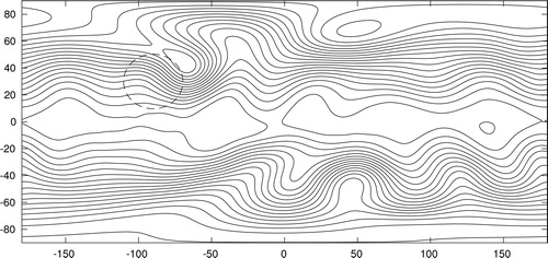The geopotential corresponding to the conical mountain is $${\Psi }_s=g{h}_{s0}(1-r/R),\text{where}{h}_{s0}=2000,R=\pi /9,$$ and $r=\min (\sqrt{{(\lambda -{\lambda }_c)}^2+{(\theta -{\theta }_c)}^2},R).$ We have computed $\Psi ={\Psi }^{*}+{\Psi }_s,$ which occurs in the two momentum equations, whereas ${\Psi }^{*}=\Psi -{\Psi }_s$ appears in the continuity equation. After an initial transient phase there seems to be fairly well-behaved solutions, but with discontinuous first order derivatives on the circle limiting the base of the mountain and thus less smooth than the Cosine bell in Section 4.2. Contour curves for the total height H are depicted in Fig. 2.

Fig. 2. Contour curves for the total height H of the fluid for the mountain problem, no. 5 from Williamson et al. (1992): n = 360, K = 3, 2p = 6, $c={10}^{-5},$ T = 15 days. Method I.

It is fairly easy to experimentally determine a ’stability interval’ $$0<c_{\mathit{min}}\le c\le c_{\mathit{max}},$$ where c_min guarantees that there is enough smoothing for stability and c_max that we stay inside the stability region of the time integrator, in the left part of the complex plane. We observe that for implicit methods c_max can be infinite. For the present example we can choose $c_{\mathit{min}}=0.1\times {10}^{-6}$ and $c_{\mathit{max}}=18\times {10}^{-6}$ for $2p=6,$ and $c_{\mathit{min}}=0.5\times {10}^{-6}$ and $c_{\mathit{max}}=140\times {10}^{-6}$ for $2p=4.$

In Table 6, the conservation properties are about the same for $2p=6$ and $2p=4,$ which is natural since they are caused by cancellation of errors in the height of the fluid rather than by accuracy. We recall that q is the number of longitudinal mesh intervals that is replaced by q−1 intervals in the following segment, cf. Section 3.2. Only q−1 interpolation formulas are required and repeated periodically. This can be seen as a more regular way to interpolate between segments than the one of method I, which has resulted in greater accuracy for the total mass. The values of c in Table 6 have been obtained by using some tests.

Table 6. Zonal flow over an isolated mountain, ${\theta }_c={30}^o,$ n = 360, K = 3, $\Delta t=300,$ T = 15 days, 6 or 4 before ${\overline{r}}_m(15)$ or ${\overline{r}}_e(15)$ denotes the approximation order.

Method	${10}^6·c$	6, ${\overline{r}}_m(15)$	6, ${\overline{r}}_e(15)$	${10}^6·c$	4, ${\overline{r}}_m(15)$	4, ${\overline{r}}_e(15)$
I	10	1.0986e-06	2.3144e-03	3	1.0277e-06	2.3085e-03
I	12	1.0977e-06	2.3143e-03	5	9.9984e-07	2.3039e-03
I	15	1.0985e-06	2.3142e-03	10	1.0358e-06	2.2925e-03
II, q = 6	0.4	3.4746e-07	2.3150e-03	1	5.5676e-07	2.3132e-03
II, q = 6	0.5	3.4208e-07	2.3150e-03	3	4.8095e-07	2.3086e-03
II, q = 6	1	3.5403e-07	2.3150e-03	5	4.8333e-07	2.3039e-03

In order to further investigate the reliability of our Equator-Pole grid systems, we have integrated the mountain problem for 5 years, using methods of order 6. In Table 7, the maximal relative errors in magnitude of the total mass appear in the fourth column and the corresponding quantity for the total energy in the last one, both after 5 years. The values of c are taken from Table 6.

Table 7. The mountain problem, ${\theta }_c={30}^o,$ n = 360, K = 3, $\Delta t=300,$ T = 5 years.

Method	2p	${10}^6·c$	$r_m(T)$	$r_e(T)$
I	6	12	$1.49·{10}^{-5}$	$1.12·{10}^{-2}$
II, q = 6	6	0.5	$0.87·{10}^{-5}$	$1.04·{10}^{-2}$

5. Summary

The Equator-Pole grid system introduced in (S-E-P), for the solution of the shallow water equations on the sphere, consists of one equatorial and two polar grids. Here we generalise this by permitting the equatorial grid to be reduced, that is divided into segments. We give two methods of reduction, called method I and method II, in Sections 3.1 and 3.2, respectively. The reduction technique seems to work quite well, as can easiest be seen in Table 4.

By using reductions the total number of grid points on the sphere can be decreased by 20% or more, and for high resolution also the computing time by a similar percentage. The change in accuracy for the height of the fluid is negligible, and for the total mass the accuracy is increasing with increased uniformity of the grid system, cf. Table 3. High uniformity might have additional advantages, for example in conjunction with comprehensive wave propagation. The different wave speeds computed will, among other things, depend on the uniformity of the grid system used and its resolution. Low uniformity or resolution might lead to interaction between waves with no analogue in the continuous model.

We have demonstrated high accuracy in the total mass for fairly simple problems, both with and without smooth solutions. For realistic NWP models the situation can be more complicated, e.g. water can contribute to the atmosphere’s mass and give rise to far less smooth problems than those considered here. We mention that Allen and Zerroukat (2015) have derived a two-dimensional generalisation of the shallow water equations, which includes moist.

We use high order centred finite difference approximations of first order spatial derivatives, in the shallow water equations. This requires only a fraction of the work per grid point compared with some other methods of the same order. This fraction decreases rapidly with the order of approximation. Further, one can very easily increase the order of approximation by increasing the order of approximation for first order derivatives. For methods of order 4, 6, 8 and 10 the corresponding spatial stencils contain only 9, 13, 17 and 21 grid points, respectively. The higher the order of the spatial approximation, up to a bound depending on the resolution, the better treatment of fronts in the solutions, see for instance Table 2 in (S-E-P). For the time integration, we have used the explicit fourth order Runge-Kutta method.

The Equator-Pole grids presented here only focus on uniformity, except in Section 3.4, and are mainly intended to be basic grid systems. To make them more flexible, for instance when taking jet streams and orography into account, they need to be modified, perhaps by using overlapping techniques.

Acknowledgements

I want to express my sincere gratitude to the anonymous reviewer for many valuable information about NWP, of which I was not aware.

Disclosure statement

No potential conflict of interest was reported by the authors.

References

- Allen, T. and Zerroukat, M. 2015. A moist Boussinesq shallow water equations set for testing atmospheric models. J. Comput. Phys. 290, 55–72.
- Allen, T. and Zerroukat, M. 2016. A deep non-hydrostatic compressible atmospheric model on Yin-Yang grid. J. Comput. Phys. 319, 44–60. doi:10.1016/j.jcp.2016.05.022
- Bao, L., Nair, R. D. and Tufo, H. M. 2014. A mass and momentum flux-form higher-order discontinuous Galerkin shallow water model on the cubed-sphere. J. Comput. Phys. 271, 224–243. doi:10.1016/j.jcp.2013.11.033
- Chen, C., Li, X., Shen, X. and Xiao, F. 2014. Global shallow water models based on multi-moment constrained finite volume method and three quasi-uniform spherical grids. J. Comput. Phys. 271, 191–223. doi:10.1016/j.jcp.2013.10.026
- Gates, W. L. and Riegel, A. 1963. A study of numerical errors in the integration of barotropic flow on a spherical grid. J. Geophys. Res. 67, 406–423.
- Giraldo, F. X. 2006. High-order triangle-based discontinuous Galerkin methods for hyperbolic equations on rotating sphere. J. Comput. Phys. 214, 447–465. doi:10.1016/j.jcp.2005.09.029
- Hortal, M. and Simmons, A. J. 1991. Use of reduced Gaussian grids in spectral models. Mon. Wea. Rev. 119, 1057–1074. doi:10.1175/1520-0493(1991)119<1057:UORGGI>2.0.CO;2
- Kageyama, A. and Sato, T. 2004. The Yin-Yang grid: an overset grid in spherical geometry. Geochem. Geophys. Geosyst. 5, 1–15.
- Kreiss, H.-O. and Oliger, J. 1972. Comparison of accurate methods for the integration of hyperbolic equations. Tellus A 24, 199–215.
- Kurihara, Y. 1965. Integration of the primitive equations on a spherical grid. Mon. Weather Rev. 95, 399–415.
- Läuter, M., Handorf, D. and Dethloff, K. 2005. Unsteady analytical solutions of the spherical shallow water equations. J. Comput. Phys. 210, 535–553. doi:10.1016/j.jcp.2005.04.022
- Läuter, M., Giraldo, F. X., Handorf, D. and Dethloff, K. 2008. A discontinuous Galerkin method for the shallow water equations using spherical triangular coordinates. J. Comput. Phys. 227, 10226–10243. doi:10.1016/j.jcp.2008.08.019
- Layton, A. T. 2002. Cubic spline collocation methods for the shallow water equations on the sphere. J. Comput. Phys. 179, 578–592. doi:10.1006/jcph.2002.7075
- Li, J. G. 2018. Shallow water equations on a spherical multiple-cell grid. Q. J. R. Meteorol. Soc. 144, 1–12. doi:10.1002/qj.3139
- Nair, R. D., Thomas, S. J. and Loft, R. D. 2005. A discontinuous Galerkin transport scheme on the cubed sphere. Mon. Wea. Rev. 133, 814–828. doi:10.1175/MWR2890.1
- Pudykiewics, J. A. 2011. On numerical solution of the shallow water equations with chemical reactions on icosahedral geodesic grid. J. Comput. Phys. 230, 1956–1991. doi:10.1016/j.jcp.2010.11.045
- Putman, W. M. and Lin, S.-J. 2007. Finite-volume transport on various cubed-sphere grids. J. Comput. Phys. 227, 55–78. doi:10.1016/j.jcp.2007.07.022
- Qaddouri, A. and Lee, V. and 2011. The Canadian global environmental multi scale model on the Yin-Yang grid system. Q. J. R. Meteorol. Soc. 137, 1913–1926. doi:10.1002/qj.873
- Ronchi, C., Iacono, R. and Paolucci, P. S. 1996. The cubed sphere: a new method for the solution of partial differential equations in spherical geometry. J. Comput. Phys. 124, 93–114. doi:10.1006/jcph.1996.0047
- Sadourny, R. 1972. Conservative finite-differencing of the primitive equations on quasi-uniform spherical grids. Mon. Wea. Rev. 100, 136–144. doi:10.1175/1520-0493(1972)100<0136:CFAOTP>2.3.CO;2
- Staniforth, A. J. and Thuburn, J. 2012. Horizontal grids for global weather and climate prediction models: a review. Q. J. R. Meteorol. Soc. 138, 1–26. doi:10.1002/qj.958
- Starius, G. 2014. A solution to the pole problem for the shallow water equations on the sphere. TWMS J. Pure Appl. Math. 5, 152–170.
- Starius, G. 2018. ‘The Equator-Pole grid system’: An overset grid system for the sphere, with an optimal uniformity property. Tellus A 70, 1–14.. doi:10.1080/16000870.2018.1541373
- Tolstykh, M. A. and Shashkin, V. V. 2012. Vorticity-divergence mass-conserving semi-Lagrangian shallow water model using the reduced grid on the sphere. J. Comput. Phys. 231, 4205–4233. doi:10.1016/j.jcp.2012.02.016
- Ullrich, P. A., Jablonowski, C. and van Leer, B. 2010. High-order finite-volume methods for the shallow-water equations on the sphere. J. Comput. Phys. 229, 6104–6134. doi:10.1016/j.jcp.2010.04.044
- Williamson, D. L. 1968. Integration of the barotropic vorticity equation on a spherical geodesic grid. Tellus 20, 642–653.
- Williamson, D. L. 2007. The evolution of dynamical cores for global atmospheric model. J. Meteorol. Soc. Jpn. 85B, 241–269. doi:10.2151/jmsj.85B.241
- Williamson, D. L., Drake, J. B., Hack, J. J., Jakob, R. and Swarztrauber, P. N. 1992. A standard test set for numerical approximation to the shallow water equations in spherical geometry. J. Comput. Phys. 102, 211–224. doi:10.1016/S0021-9991(05)80016-6