Development of the tangent linear and adjoint models of the MPAS-Atmosphere dynamic core and applications in adjoint relative sensitivity studies

Abstract

This study develops and tests a version of the Python-driven, non-hydrostatic Model for Prediction Across Scales – Atmosphere (MPAS-A) dynamic model, as well as its tangent linear and adjoint models. The non-linear, non-hydrostatic dynamic core of the MPAS-A is restructured to have a Python driver for the convenience of parsing namelists, manipulating matrices, controlling simulation time flows, reading model inputs, and writing outputs, while the heavy-duty mediation and model layers are retained in Fortran for computational efficiency. Under the same Python-driving structure, developed are the tangent linear and adjoint models for the dynamic core of the MPAS-A model with verified correctness. The case of Jablonowski and Williamson’s baroclinic wave is used for demonstrating the approximation accuracy of the MPAS-A tangent linear model and the applicability of the MPAS-A adjoint model to relative sensitivity studies. Numerical experimental results show that the tangent linear model can well approximate the temporal evolutions of non-linear model perturbations for all model variables over a four-day forecast period. Employing the MPAS-A adjoint model, it is shown that the most sensitive regions of the 24-h forecast of surface pressure are weather dependent. An interesting westward vertical tilting is also found in the relative sensitivity results of a 24-h forecast of surface pressure at a point located within a trough to model initial conditions. This functionality of the MPAS-A adjoint model is highly essential in understanding dynamics and variational data assimilation.

Plain Language Summary

The MPAS-A is an advanced global numerical weather prediction model with a hexagonal mesh that can be compressed for higher resolutions in some targeted regions of interest and smoothly transitioned to coarse resolutions in others. In this study, a Python-driven MPAS-A model is first developed, combining a flexible Python driver and Fortran’s fast computation, making the MPAS-A model exceedingly user- and platform-friendly. The tangent linear and adjoint models of the MPAS-A dynamical core are then developed, both of which are required for various sensitivity studies. They are also indispensable components of a future MPAS-based global four-dimensional variational (4D-Var) data assimilation system. Finally, the relative sensitivity of a baroclinic instability wave development is obtained and shown using the MPAS-A adjoint model.

Keywords:

• MPAS-Atmosphere, tangent linear, adjoint model, sensitivity analysis, NWP

Key Points

• A Python-driven MPAS-A dynamic-core-only is tested

• The tangent linear and adjoint models of the MPAS-A are developed and their correctness is verified

• The relative sensitivities obtained by using the MPAS adjoint model shows interesting results for a baroclinic instability test case

1. Introduction

Numerically solving atmospheric dynamical and physical equations has been the primary approach for making weather forecasts. The increasing computational capabilities allow for resolving atmospheric motions at finer and finer scales. Nonetheless, simulations permitting non-hydrostatic scales everywhere on the globe are still challenging and highly expensive (Satoh et al., 2008). An alternative solution is offered by the Model for Prediction Across Scales – Atmosphere (MPAS-A), which employs finite-volume irregular centroidal Voronoi meshes on a C-grid with an option of smoothly varying resolutions (Ringler et al., 2008; Skamarock et al., 2012; Park et al., 2013). Under the framework of MPAS-A, regions of interest may be covered with grids of the highest possible resolution and the remaining part of the globe with coarser grids and smooth transitions from high to coarse resolutions. Hagos et al. (2013) examined and compared the error characteristics of such smoothly varying, variable-resolution meshes in MPAS-A to those from a two-way nesting approach in the Weather Research and Forecasting (WRF) model. It was found that errors appeared near the edges of high-resolution nesting regions in WRF simulations but were avoided by the variable-resolution meshes in MPAS-A. Rauscher and Ringler (2014) showed that the regionally refined mesh of MPAS-A helps to resolve mid-latitude eddy activities that are often induced by orography, land–sea contrasts and sea surface temperature anomalies.

In addition to an advanced numerical forecast model, a complete and modern numerical weather prediction system also encompasses a data assimilation procedure to produce the optimal initial conditions for making forecasts. Atmospheric data assimilation problems, in general, involve large dimensions. The introduction of adjoint techniques into data assimilation has drastically reduced computational costs as well as opened new opportunities in meteorological research areas (Le Dimet and Talagrand, 1986; Courtier and Talagrand, 1990; Rabier et al., 1992, 1996; Courtier et al., 1993, 1994). Based on the Penn State – NCAR Mesoscale Model (MM5), Zou et al. (1995) developed the adjoint model of MM5 to formulate the four-dimensional variational (4D-Var) assimilation system and found significant positive impacts on short-range forecasts after assimilating rainfall observations (Zou and Kuo, 1996). Similarly, aimed at building a WRF-based 4D-Var assimilation system, Xiao et al. (2008) developed the tangent linear (TL) and adjoint (AD) models of the WRF model, with the aid of an automatic differentiation tool (Giering and Kaminski, 2003), and showed that adjusting initial conditions using the WRF adjoint model could significantly improve the Antarctic windstorm forecast. In addition to its essential role in variational data assimilation, adjoint models also have remarkable and versatile potentials in other meteorological applications. Many questions posed in the field of atmospheric science involve sensitivities. An example is how some weather features of interest may change if certain small perturbations are added to the initial conditions. Traditionally, answering these questions would involve multiple model runs with sequentially perturbed components in an initial condition vector. By contrast, with the aid of adjoint models, a comprehensive sensitivity field at the model starting time can be obtained with a single adjoint model run. Errico (1997) and Zou et al. (1997) comprehensively described the applicability of adjoint models in various topics, including parameter estimation, model stability analysis and synoptic studies.

During the last few years, the programming language Python has become increasingly popular among atmospheric science researchers as well as those from other Earth science disciplines (Lin, 2012). Due to its concise and natural syntax, programmes written in Python are clear and easy to read. Well-developed packages are readily available to handle input/output (IO) tasks in various encoding formats commonly seen in the field of Earth science, such as Gridded Binary, Network Common Data Form, Hierarchical Data Format (HDF) 4 and HDF5. In tasks involving modelling, the handling of date and time is also frequently dealt with, which is also made exceedingly simple in Python (Lutz, 2013). Nonetheless, Python comes with disadvantages, including much slower computational speeds than compiled programming languages like Fortran. In this study, the driver layer of the non-linear MPAS-A is redeveloped in Python to control the simulation workflow, including IO, date and time in model simulations to reconcile the advantages and disadvantages of both Python and Fortran. The heavy-duty dynamical calculations are retained in Fortran so that the model’s computational speed is hardly compromised. Such a structural arrangement makes the installation, compilation and modification of the model even more user- and platform-friendly than without using the Python driver. As this research involves only the dynamical core of the MPAS-A without moist physics for the moment, conducted are numerical experiments with the baroclinic wave case of Jablonowski and Williamson (JW), a case commonly adopted for testing the performance and stability of numerical weather prediction (NWP) models’ dynamical cores in numerous previous studies (Jablonowski and Williamson, 2006a, 2006b; Park et al., 2013). Section 2 briefly introduces some technical features of the non-hydrostatic MPAS-A model and the redeveloped Python driver layer. Section 3 presents the development of the TL model using the same combined Python–Fortran structure and tests its correctness. Section 4 involves the development of correctness checks of the MPAS-A adjoint model, and Section 5 presents some results from two adjoint relative sensitivity studies. Section 6 gives a summary and conclusions.

2. A brief description of the MPAS atmospheric solver and case selection

The MPAS is a global modelling system that uses spherical centroidal Voronoi tessellations discretization, allowing for both quasi-uniform and smoothly variable horizontal resolution meshes. The MPAS framework houses multiple geophysical dynamical solvers, including the atmosphere, ocean, sea ice and land ice. MPAS-A is a compressible, non-hydrostatic atmospheric model. The variable-resolution-permitting centroidal mesh is suitable for regional NWPs and regional climatological studies over high-resolution regions (Skamarock et al., 2012; Hagos et al., 2013; Park et al., 2013). Figure 1 is an example of a refined circular area centred at [50° N, 170° W] with a horizontal resolution of about 25 km between neighbouring cell centres, which progressively becomes coarser and coarser to 92 km in remote parts of the globe. Figure 1b demonstrates the actual distributions of centroidal grid cells within the transitional region indicated by a white box in Fig. 1a. The mesh with gradually varying resolutions is to be contrasted with the traditionally two-way nested grids (Skamarock and Klemp, 2008). In the settings of nested grids, horizontal resolutions change abruptly over the boundaries of the refined areas, possibly generating additional systematic errors in the simulation results (Hagos et al., 2013).

Fig. 1. (a) Global distribution of distances between neighbouring cells (shaded in colour) of a variable resolution grid with horizontal resolutions ranging from 25 km to 92 km. The centre of refined resolution is at [50° N, 170° W]. (b) Cell distribution of variable resolution grid cells within a zoomed region indicated by the white box in (a). The area in (a) is shown using the equidistant conic projection, and the area in (b) is shown using the equidistant cylindrical projection.

The MPAS-A inherited the approach of the Advanced Research WRF (ARW) for solving the non-hydrostatic dynamical and physical equations, including the staggered C-grid spatial discretization and the third-order Runge–Kutta temporal integration scheme. In addition to the Runge–Kutta scheme, also adopted is a time-splitting technique to integrate gravity and acoustic waves. Spatially, the vertical coordinate in the MPAS-A model is terrain-following and height-based, different from the ARW. The MPAS-A model has five prognostic state variables, i.e. horizontal momentum (u) perpendicular to the cell edges; coupled potential temperature (θ), coupled density (ρ) and specific humidity (q) residing at the cell centres; and vertical momentum (w) located at the cell centres horizontally but between layers vertically. Ringler et al. (2008) and Skamarock et al. (2012) provided more details about the unstructured centroidal mesh and MPAS-A dynamics solver, respectively.

In this study, the MPAS-A is restructured so that the driver layer is written in Python, and the mediation and model layers are retained in Fortran, in which the model layer is where the actual dynamical computations take place and the mediation layer is an intermediate layer of the software placed between the driver and model layers. Under this framework, the functionalities in the driver layer, including installation, compilation, controlling of the simulation time flow and IO, are made exceedingly user- and platform-friendly (see Appendix A), which will also be the case for a prospective 4D-Var assimilation system. The fast computation efficiency of Fortran is maintained under the Python-driving framework since the heavy-duty mediation and model layers are still written in Fortran. The Python intrinsic utility F2Py, i.e. Fortran to Python interface generator, builds the interfaces between the Python driver layer and Fortran mediation/model layers, which compiles Fortran codes with common Fortran compilers (e.g. gfortran, ifort and pgfortran), providing a connection between the two programming languages (Peterson, 2009). In this study, the TL/AD Fortran programmes are developed line-by-line manually following the guidance detailed in the work by Zou et al. (1997), without using any automatic differentiation tool. Under this Python-driving structure, the non-linear forward, TL, and adjoint models of the MPAS-A performs simulations exactly like the original MPAS-A, regardless of the types of meshes chosen in different numerical experiments.

The JW test case is adopted in this research to test the simulation performances of the MPAS-A non-hydrostatic dynamical core with both quasi-uniform and variable-resolution meshes as well as those of the accuracy of both the TL and adjoint models. For a demonstration of the benefits from the smooth variable-resolution mesh, conducted are three separate numerical experiments with the same Python-driving MPAS-A dynamical core and the same initial conditions but with three different meshes: (1) uniform resolution (UR) at 120 km with 40,962 cells, (2) UR at 30 km with 655,362 cells and (3) variable resolution (VR) ranging from 25 to 92 km with 163,842 cells (Fig. 1a). Starting with the initial conditions of the baroclinic instability test case, the model integrates for a period of nine days. Figure 2 shows the surface pressure features of an evolving baroclinic wave on day 9 from the UR-120-km and UR-30-km experiments and their differences. While the patterns in Fig. 2a,b are similar, differences in the magnitude of surface pressure exceed 15 hPa in places. Figure 3a shows the wave features on day 9 from the VR experiment. As described earlier, the area with the finest resolution is centred at [50° N, 170° W], where most of the wave patterns may be well confined in finer resolutions, guided by the black contours. Comparing results from the VR experiment (Fig. 3a) and from the UR-30-km experiment (Fig. 2b), differences (Fig. 3b) are noticeably smaller than those between the UR-120-km and UR-30-km experiments (Fig. 2c). As indicated by the number of grid cells, the MPAS-A loops through the VR mesh consists of only 25% of the number of cells in the UR-30-km mesh, which is a direct indicator of a significant saving in the computational cost. In reality, for 24-h forecasts with the same integration time step (150 sec), the VR experiment took only 16% of the computational time of the UR-30-km experiment (Table 1). This implies that for a given region of interest, the smoothly variable resolution offered in the MPAS-A may help to achieve high-resolution simulation performances for only a fraction of the computational cost of an experiment with a high-resolution uniform mesh.

Fig. 2. Surface pressure distributions (unit: hPa) after nine-day integrations with uniform resolutions of (a) 120 km and (b) 30 km. (c) Differences in surface pressure between the 120 and 30 km resolutions.

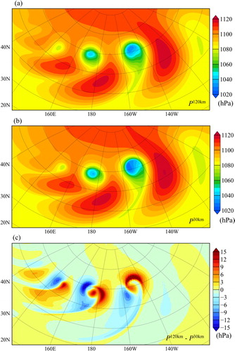
Fig. 3. (a) Surface pressure distribution (unit: hPa) after a nine-day integration with a variable resolution. (b) Differences in surface pressure between the variable-resolution and 30-km uniform resolutions. Point A is at [61° N, 153° W], and point B is at [80° N, 153° W]. The black contours are the distances (unit: km) between neighbouring cells shown in Fig. 1a.

Table 1. Computational costs for 24-h integrations of a global MPAS-A non-linear model at 120-km and 30-km quasi-uniform resolutions and a variable resolution varying from 25 km to 92 km, as well as the costs for tangent linear and adjoint models at the variable resolution.

Model	Resolution (km)	Cost (h)	Time step (sec)
Non-linear	120	0.24	450
	30	17.5	150
	25–92	2.8
Tangent linear	25–92	5.39
Adjoint	25–92	12.5

3. Development of the MPAS-A TL model

The non-hydrostatic MPAS-A can be symbolically written as (1) $$\mathbf{x}\left(t_r\right)={\mathcal{M}}_{\mathbf{r}}\left({\mathbf{x}}_0\right),$$(1) where t_r denotes the forecast time and t₀ the initial time, vector x represents all five model prognostic variables, ${\mathcal{M}}_{\mathrm{r}}$ is the non-linear forward model operator, and x₀ represents the initial conditions for the forecast model. The TL model can be obtained by linearizing ${\mathcal{M}}_{\mathrm{r}}$ with respect to all model prognostic and diagnostic variables, expressed as (2) $$\Delta \mathbf{x}\left(t_r\right)={\mathbf{M}}_{\mathrm{r}}\left({\mathbf{x}}_0\right)\Delta {\mathbf{x}}_0=\frac{\partial {\mathcal{M}}_r\left({\mathbf{x}}_0\right)}{\partial \mathbf{x}}\Delta {\mathbf{x}}_0,$$(2) where the prefix $\Delta$ denotes perturbations to the corresponding non-linear state variables x, and M_r is the TL model operator. Table 1 lists the time it takes to complete a 24-h simulation with the TL model. The TL model requires slightly less than three times the cost of the non-linear forward model, the reason being that after each calculation of a linearized equation, the original non-linear equation will also be calculated to update the non-linear trajectory that the TL model is linearized on.

The correctness of the MPAS-A TL model can be verified by checking whether the following equation is satisfied: (3) $$\Phi \left(\alpha \right)=\frac{\Vert {\mathcal{M}}_r({\mathbf{x}}_0+\alpha \mathbf{h})-{\mathcal{M}}_r\left({\mathbf{x}}_0\right)\Vert }{\Vert {\mathbf{M}}_r\alpha \mathbf{h}\Vert }=1+O\left(\alpha \right).$$(3)

Conducted was a set of five experiments with a 24-h integration period for the TL correctness check. In the first four tests, each model prognostic variable, i.e. 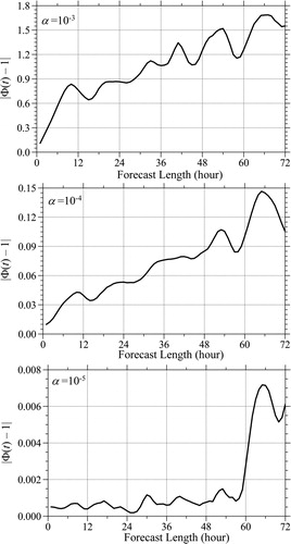u, w, ρ and θ, in vector h in Equation (3)(3) $$\Phi \left(\alpha \right)=\frac{\Vert {\mathcal{M}}_r({\mathbf{x}}_0+\alpha \mathbf{h})-{\mathcal{M}}_r\left({\mathbf{x}}_0\right)\Vert }{\Vert {\mathbf{M}}_r\alpha \mathbf{h}\Vert }=1+O\left(\alpha \right).$$(3) was separately assigned non-zero values. In the fifth experiment, all four prognostic variables in vector h were simultaneously assigned non-zero values. As the scale factor α becomes smaller and smaller, the function Φ(α) is expected to approach unity in an approximately linear way. Figure 4 shows the results of the correctness tests. As anticipated, the values of Φ(α) progressively become closer and closer to unity as the scale factor α gets smaller and smaller for certain ranges of α values in each of the testing experiments. When α is too small, the accuracies of the Φ(α) values start to be affected by the machine round-off errors and drift away from unity. Figure 5 shows the temporal evolutions of Φ(α) with an integration period of 72 h when α equals to 10⁻³, 10⁻⁴ and 10⁻⁵. In all three cases, the values of |Φ(α) – 1| gradually increase as time moves on. However, the approximations of perturbation evolutions by the TL model are noticeably better when the initial perturbation sizes are small (α = 10⁻⁵, Fig. 5c) than when perturbation sizes are relatively big (α = 10⁻³, Fig. 5a).

Fig. 4. Variations in the function |Φ(α) – 1| for the correctness check of the MPAS-A tangent linear model for the 24-h forecast length when the initial conditions for variables u, w, ρ and θ are separately perturbed, where α is the scale factor of initial perturbations.

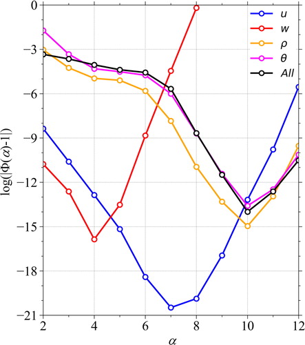
Fig. 5. Temporal evolutions of the global mean |Φ(t) – 1| with respect to the forecast length when α = 10^–3, 10^–4 and 10^–5.

A separate set of experiments is included following Equation (3)(3) $$\Phi \left(\alpha \right)=\frac{\Vert {\mathcal{M}}_r({\mathbf{x}}_0+\alpha \mathbf{h})-{\mathcal{M}}_r\left({\mathbf{x}}_0\right)\Vert }{\Vert {\mathbf{M}}_r\alpha \mathbf{h}\Vert }=1+O\left(\alpha \right).$$(3) , in which both x and h in Equation (3)(3) $$\Phi \left(\alpha \right)=\frac{\Vert {\mathcal{M}}_r({\mathbf{x}}_0+\alpha \mathbf{h})-{\mathcal{M}}_r\left({\mathbf{x}}_0\right)\Vert }{\Vert {\mathbf{M}}_r\alpha \mathbf{h}\Vert }=1+O\left(\alpha \right).$$(3) were given the values of the simulation results on day 5 of the JW baroclinic wave case, and α is set as 10⁻³ (Fig. 6). After a four-day integration, the simulation results reach the same time as the results shown in Figs. 2 and 3, i.e. day 9. Figure 7a shows the differences between the two non-linear model simulations calculated with the MPAS dynamic core only, i.e. $\Vert {\mathcal{M}}_r(\mathbf{x}+\alpha \mathbf{h})-{\mathcal{M}}_r\left(\mathbf{x}\right)\Vert$ in Equation (3)(3) $$\Phi \left(\alpha \right)=\frac{\Vert {\mathcal{M}}_r({\mathbf{x}}_0+\alpha \mathbf{h})-{\mathcal{M}}_r\left({\mathbf{x}}_0\right)\Vert }{\Vert {\mathbf{M}}_r\alpha \mathbf{h}\Vert }=1+O\left(\alpha \right).$$(3) , and Fig. 7b shows the results from the TL model taking αh as input, i.e. ${\mathbf{M}}_r(\mathbf{x})\alpha \mathbf{h}$ in Equation (3)(3) $$\Phi \left(\alpha \right)=\frac{\Vert {\mathcal{M}}_r({\mathbf{x}}_0+\alpha \mathbf{h})-{\mathcal{M}}_r\left({\mathbf{x}}_0\right)\Vert }{\Vert {\mathbf{M}}_r\alpha \mathbf{h}\Vert }=1+O\left(\alpha \right).$$(3) . Both results appear almost identical, indicating a close approximation of the TL model forecast to the evolution of perturbations as the non-linear model differences. Figure 7c shows pixel-by-pixel comparisons of the results in Fig. 7a,b, suggesting a high correlation between the two, with a root-mean-square error of 0.00454 hPa in the linear regression fit.

Fig. 6. (a) ρ, (b) θ, (c) u and (d) w and surface pressure (black contours, unit: hPa) at 0000 UTC of day 5 with the variable resolution mesh.

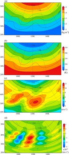
Fig. 7. (a) Differences in surface pressure (unit: hPa) after four-day integrations of the non-linear forward model with and without perturbations [i.e. ${\mathcal{M}}_{\mathrm{r}}$(x + αh) – ${\mathcal{M}}_{\mathrm{r}}$(x)], and (b) the four-day perturbation forecast of the tangent linear model [M(x)αh], where a perturbation of α = 10^–3 is given to all state variables (u, w, ρ, θ, and q_v) on day 5, as shown in Fig. 6. Surface pressures from the non-linear forward model on day 9 are shown in (a) and (b) as black contours. (c) Scatter plot of M(x)αh as a function of [${\mathcal{M}}_{\mathrm{r}}$(x + αh) – ${\mathcal{M}}_{\mathrm{r}}$(x)]. The linear fit is y = 0.983x + 0.0179, with a root-mean-square error of 0.00454 hPa.

4. Development of the MPAS-A adjoint model

The MPAS-A adjoint model is essentially the transpose of the MPAS-A TL model, expressed as (4) $$\Delta {\widehat{\mathbf{x}}}_0={\mathbf{M}}_r^T\left(\mathbf{x}\right)\Delta \widehat{\mathbf{x}}\left(t_r\right),$$(4) where $\Delta \widehat{\mathbf{x}}$ denotes the adjoint variable, and t_r is the final time of interest. Table 1 shows the time it takes for the MPAS-A adjoint model to generate a 24-h simulation. Because the adjoint model performs calculations backward in time, the non-linear prognostic and intermediate diagnostic variables still need to be updated forward in time. Thus, the scheme adopted in the MPAS-A adjoint model is that the prognostic variables at every time step are stored while the diagnostic variables within each individual time step are recalculated during the process of adjoint calculations, which is the reason why the adjoint model takes more time than the TL model.

The correctness of the MPAS-A adjoint model can be verified based on the following equation: (5) $$〈\Delta {\mathbf{x}}_2,{\mathbf{M}}_r\Delta {\mathbf{x}}_1〉=〈{\mathbf{M}}_r^T\Delta {\mathbf{x}}_2,\Delta {\mathbf{x}}_1〉.$$(5)

The left-hand side (LHS) of Equation (5)(5) $$〈\Delta {\mathbf{x}}_2,{\mathbf{M}}_r\Delta {\mathbf{x}}_1〉=〈{\mathbf{M}}_r^T\Delta {\mathbf{x}}_2,\Delta {\mathbf{x}}_1〉.$$(5) is the inner product of the TL model forecast at time t_r from an initial condition $\Delta {\mathbf{x}}_1$ at time t₀, i.e. $\Delta \mathbf{x}(t_r)={\mathbf{M}}_r\Delta {\mathbf{x}}_1,$ with a vector $\Delta {\mathbf{x}}_2,$ and the right-hand side (RHS) is the inner product of $\Delta {\mathbf{x}}_1$ with the output of the adjoint model integration from the time t_r to t₀, i.e. $\Delta {\widehat{\mathbf{x}}}_0={\mathbf{M}}_r^T\Delta {\mathbf{x}}_2.$ If the adjoint model is developed correctly, the LHS and RHS of Equation (5)(5) $$〈\Delta {\mathbf{x}}_2,{\mathbf{M}}_r\Delta {\mathbf{x}}_1〉=〈{\mathbf{M}}_r^T\Delta {\mathbf{x}}_2,\Delta {\mathbf{x}}_1〉.$$(5) is expected to agree with the machine accuracy of the data type declared in the program, which is double precision in the MPAS-A, for any vectors of $\Delta {\mathbf{x}}_1$ and $\Delta {\mathbf{x}}_2.$ Following Equation (5)(5) $$〈\Delta {\mathbf{x}}_2,{\mathbf{M}}_r\Delta {\mathbf{x}}_1〉=〈{\mathbf{M}}_r^T\Delta {\mathbf{x}}_2,\Delta {\mathbf{x}}_1〉.$$(5) , the first set of five experiments is included with the integration time t_r equal to 1, 3, 6, 9 and 12 h with $\Delta {\mathbf{x}}_1={10}^{-3}{\mathbf{x}}_0$ and $\Delta {\mathbf{x}}_2={\mathbf{M}}_r\Delta {\mathbf{x}}_1.$ The second set of testing experiments is the same as the first set except for changing $\Delta {\mathbf{x}}_2$ to the 48-h non-linear model forecasts ${\mathcal{M}}_{\mathrm{r}}$_48h(x₀). The resulting LHS and RHS from the five tests of both sets agree with the precision of machine accuracies, indicating the correctness of the MPAS-A adjoint model (Table 2).

Table 2. Correctness check results of the newly developed MPAS-A adjoint model when it is integrated for 1, 3, 6, 9 and 12 h.

Time (h)	LHS	RHS	(LHS – RHS)/LHS
Δx1 = 10^–3x0 and Δx2 = MrΔx1
1	97.20768296905979	97.20768296905982	2.9238130734430064 × 10^–16
3	84.96752467420752	84.96752467420744	1.003502557219898 × 10^–15
6	48.355553249923005	48.35555324992303	4.4082386903177345 × 10^–16
9	76.02678600397633	76.02678600397634	1.8691905132565715 × 10^–16
12	111.59107980162807	111.59107980162807	0.0
Δx1 = 10^–3x0 and Δx2 = ${\mathcal{M}}_{\mathrm{r}}$48h(x0)
1	15099708.797756858	15099708.79775685	4.934254492398325 × 10^–16
3	15693692.520537037	15693692.5205371	4.0353750394292416 × 10^–15
6	16099500.125983704	16099500.125983633	4.396441822224065 × 10^–15
9	15902734.410095675	15902734.41009571	2.2254196619746773 × 10^–16
12	15704266.188497595	15704266.18849758	9.488607117957435 × 10^–16

LHS: left-hand side of Equation (5)(5) $$〈\Delta {\mathbf{x}}_2,{\mathbf{M}}_r\Delta {\mathbf{x}}_1〉=〈{\mathbf{M}}_r^T\Delta {\mathbf{x}}_2,\Delta {\mathbf{x}}_1〉.$$(5) ; RHS: right-hand side of Equation (5)(5) $$〈\Delta {\mathbf{x}}_2,{\mathbf{M}}_r\Delta {\mathbf{x}}_1〉=〈{\mathbf{M}}_r^T\Delta {\mathbf{x}}_2,\Delta {\mathbf{x}}_1〉.$$(5) .

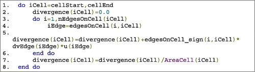
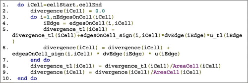
A brief example of the coding in the restructured Python–Fortran MPAS-A, as well as how divergence is calculated under the Voronoi mesh in MPAS with its corresponding TL/AD can be found in Appendices A and B, respectively. The naming convention for a given prognostic or diagnostic variables in the MPAS-A model, such as ‘divergence’, is ‘divergence_tl’ and ‘divergence_ad’ in the TL and adjoint models, respectively. The divergence at a cell centre can be found with a summation of wind vectors at all edges of the cell. All other quantities in the atmospheric dynamical equations have also been converted similarly in the TL/AD Fortran codes. Following the MPAS-A Fortran code, the TL and adjoint models are finally developed.

5. MPAS-A adjoint sensitivity analysis

An advantageous application of the adjoint model is sensitivity analysis (Errico and Vukicevic, 1992; Errico, 1997; Zou et al., 1997). A given quantity of interest (J) at the model forecast time, such as mean squared error (MSE), vorticity, surface pressure etc., can be denoted as (6) $$J=J\left({\mathbf{x}}_{t_r}\right),$$(6) where ${\mathbf{x}}_{t_{{}^r}}$ is the prognostic variables at the forecast time, or MPAS-A model output, and J is a scalar. J is also called the response function and can be the value of a variable at a single point, over a specific region, or over the entire globe. As in the case of variational data assimilation, the response function J is the MSEs between observations and model simulations. Studies are often interested in the sensitivities of a response function at the forecast time to the initial conditions, i.e. model input. Most previous research has attempted to obtain information about sensitivities by comparing the resulting response function with a slightly perturbed initial condition,$J({\mathbf{x}}_0+\Delta {\mathbf{x}}_0),$ to the response function from a control experiment, $J({\mathbf{x}}_0).$ The sensitivity of J to the initial condition may then be expressed as (7) $$\Delta J\approx \sum _k\frac{\partial J}{\partial x_{t_r,k}}\Delta x_{t_r,k},\mathrm{ }\Delta x_{t_r,j}\approx \sum _k\frac{\partial x_{t_r,j}}{\partial x_{0,k}}\Delta x_{0,k}.$$(7)

The limitations of this method are: (1) the magnitudes of the perturbation in the initial conditions have to be sufficiently small to ensure a good approximation of the gradients of J with respect to the perturbed variable$\Delta x_{0,k},$ and (2) many model runs are required to find a comprehensive profile of J’s sensitivities to all of the variables at various geographical locations. By contrast, the sensitivities of the response functions with respect to the model variables may be expressed as (Errico, 1997) (8) $$\frac{\partial J}{\partial x_{0,j}}=\sum _k\frac{\partial x_{t_r,k}}{\partial x_{0,j}}\frac{\partial J}{\partial x_{t_r,k}}.$$(8)

Compared with the term $\frac{\partial x_{t_r,j}}{\partial x_{0,k}}$ in Equation (7)(7) $$\Delta J\approx \sum _k\frac{\partial J}{\partial x_{t_r,k}}\Delta x_{t_r,k},\mathrm{ }\Delta x_{t_r,j}\approx \sum _k\frac{\partial x_{t_r,j}}{\partial x_{0,k}}\Delta x_{0,k}.$$(7) , the term $\frac{\partial x_{t_r,k}}{\partial x_{0,j}}$ in Equation (8)(8) $$\frac{\partial J}{\partial x_{0,j}}=\sum _k\frac{\partial x_{t_r,k}}{\partial x_{0,j}}\frac{\partial J}{\partial x_{t_r,k}}.$$(8) is the transpose representing the adjoint model. Note that the sensitivities of J, calculated using a single adjoint model run, are (1) independent from the perturbation sizes and (2) with respect to all model variables over the entire model domain in the initial conditions.

In the experiments of this study, the response function in the adjoint sensitivity analysis is defined as the surface pressure at two individual points, A and B, on day 9, as marked in Fig. 3a: (9) $$J\left({\mathbf{x}}_{t_r}\right)=P_{\text{surf},\mathrm{ }m}^{},\mathrm{ }m=\mathrm{A}\mathrm{ }\text{or}\mathrm{ }\mathrm{B},$$(9) where point A has the minimum surface pressure, and point B experiences calm weather throughout the simulation period. Calculated with the MPAS-A adjoint model were the sensitivities of the response function to model input variables for up to 24 h prior to day 9. The magnitudes of different model variables, as well as those of the sensitivities of J to different model variables, can vary dramatically. The concept of non-dimensional relative sensitivities is thus adopted, following the equation below (Zou et al., 1993; Carrier et al., 2008): (10) $$S_{\text{rel}}=\frac{\mathbf{x}\odot \widehat{\mathbf{x}}}{J}=\frac{1}{J}\left(\begin{array}{c}{x}_1{\widehat{x}}_1\\ x_2{\widehat{x}}_2\\ ⋮\\ x_N{\widehat{x}}_N\end{array}\right).$$(10) where x denotes non-linear state variables, $\widehat{\mathbf{x}}$ represents MPAS-A adjoint model results, J is the value of the response function and $\widehat{\mathbf{x}}.$ ⊙ represents the Hadamard product, which is defined as a vector of the same dimension as the vectors x and $\widehat{\mathbf{x}}$ consisting of the product of the ith element of x and the ith element in $\widehat{\mathbf{x}}.$ The magnitudes of the relative sensitivities found following Equation (10)(10) $$S_{\text{rel}}=\frac{\mathbf{x}\odot \widehat{\mathbf{x}}}{J}=\frac{1}{J}\left(\begin{array}{c}{x}_1{\widehat{x}}_1\\ x_2{\widehat{x}}_2\\ ⋮\\ x_N{\widehat{x}}_N\end{array}\right).$$(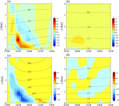10) are direct indicators of the significance of each model variable on the response function. Thus, the sensitivity results generated from the MPAS-A adjoint model may be compared across different model variables. Figure 8 shows the 12- and 24-h relative sensitivities of the surface pressure at point A in Fig. 3a with respect to ρ at the surface. Twelve or twenty-four hours prior to 0000 UTC on day 9, low-pressure centres were still to the southwest of point A. The response function is most sensitive in upstream regions following the isobars, with 24-h sensitivity results further away along and across the isobars. In comparison, Fig. 9 shows the 12- and 24-h relative sensitivities of the surface pressure at point B to ρ at the surface. At point B, no significant weather took place during the 24-h period prior to day 9. Thus, regions of sensitivity are confined to near point B. The magnitudes of the relative sensitivities in Fig. 9 are also smaller than those in Fig. 8. Figure 10 presents vertical cross-sections of the relative sensitivities with respect to ρ and zonal winds along the magenta lines in Figs. 8b and 9b. For the case of point A, shown in the left panels, the relative sensitivities in both the ρ and wind fields display a westward vertical tilting. The relative sensitivities to density (×10⁻³) are two orders of magnitude greater than those to the winds (×10⁻⁵), implying that the changes in surface pressure at point A on day 9 are significantly more sensitive to ρ than to winds in the model input 24 h prior. Similar results are seen for the relative sensitivities of the surface pressure at point B to both ρ and wind variables 12–24 h earlier. As seen in Fig. 9, the vertical distributions of ρ and wind are stably stratified.

Fig. 8. Relative sensitivities of the surface pressure at point A at 0000 UTC of day 9 (see Fig. 3a) to the ρ field at the surface level at (a) 1200 UTC and (b) 0000 UTC of day 8 (shaded in colour, ×10^–3). Black contours show the surface pressures at 1200 UTC and 0000 UTC of day 8 in (a) and (b), respectively.

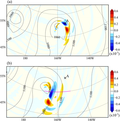
Fig. 9. Relative sensitivities of the surface pressure at point B at 0000 UTC of day 9 (see Fig. 3a) to the ρ field at the surface level at (a) 1200 UTC and (b) 0000 UTC of day 8 (shaded in colour, ×10^–3). Black contours show the surface pressures at 1200 UTC and 0000 UTC of day 8 in (a) and (b), respectively.

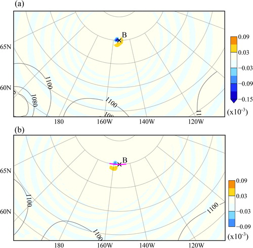
Fig. 10. Cross-sections of relative sensitivities of the surface pressure at point A (left panels) and point B (right panels) at 0000 UTC of day 9 (see Fig. 3a) to (a, b) the ρ field (×10^–3) and (c, d) the u field (×10^–5) at 0000 UTC of day 8 (shaded in colour). The ρ field at 0000 UTC of day 8 is shown in (a, b) (black curves), and the u field at 0000 UTC of day 8 is shown in (c, d) (black curves).

The adjoint sensitivity results in the experiments discussed above serve as a preliminary example for the strength of the MPAS-A adjoint model, which can efficiently help to find the areas and fields in the initial conditions that have the greatest impacts on a given scalar of interest in the forecasts. The sensitivity field shows a strong dependence on the state flow near the point of interest, which also implies the reason that flow-dependent perturbations are implicitly accounted for in 4D-Var assimilation systems. Similar applications can readily be inferred such as finding the sensitivity field of the vorticity or central surface pressure at a preceding time in a tropical cyclone case.

6. Summary and conclusions

The weather forecast capabilities over the advanced irregular centroidal mesh offered by the MPAS-A is unique for weather and climate research. In this study, the MPAS-A is restructured in such a way that the driver layer is developed in Python for its versatility and convenience when controlling the workflow of the model and that the mediation and model layers are retained in Fortran for its efficient computational speed. In the case of the Jablonowski and Williamson baroclinic wave, compared are the simulation results from the experiments using the Python-driving MPAS-A with both quasi-uniform and variable-resolution meshes. High-resolution simulation performances over regions of interest can be achieved using the variable-resolution mesh for a small fraction of the computational cost compared to using the global uniformly high-resolution mesh.

An adjoint model is a remarkably versatile tool for various sensitivity-involved meteorological research topics and serves a vital role in a four-dimensional variational assimilation system. The tangent linear (TL) and adjoint models of the MPAS-A dynamical core are developed under the same Python-driving framework in this research. Necessary correctness verification procedures are carried out and passed to ensure that both the TL and adjoint models generate accurate results. The TL model closely approximates the evolutions of perturbations after a four-day forecast when compared with the simulation differences between the perturbed and original non-linear MPAS-A model. Additional experiments are included to demonstrate the applicability of the MPAS-A adjoint model in efficiently calculating sensitivities of a given quantity of interest at forecast time, or the so-called response function, to the initial conditions or forecast model inputs. Specifically, the relative sensitivities of the surface pressure on day 9 at two separate locations, one at the centre of a low-pressure system (point A) and the other in a fair-weather region (point B), to the model variables 12 and 24 h earlier than day 9 are calculated with the adjoint model. The surface pressure at point A is primarily sensitive to areas upstream of the isobars near the centre of the low-pressure system horizontally and exhibits a westward vertical tilting. By comparison, with calm weather at point B, areas showing significant sensitivities are located near point B, regardless of the simulation time.

The physical options currently available in the MPAS-A model can readily be inserted into the Python–Fortran structure proposed in this study. Future research efforts will focus on first developing an MPAS TL/AD system with moist physics and planetary boundary layer physics parameterization schemes and then building a comprehensive global 4D-Var assimilation system.

Acknowledgements

The authors thank NCAR for releasing the source code of MPAS-Atmosphere at https://mpas-dev.github.io/. The data used to plot the results shown in this study are available at http://www.xiaoxutian.com/MPAS-Adjoint-Sensitivity/.

Appendix A

An (incomplete) example of the Python driver layer for the non-linear forward MPAS-A model is given here:

 

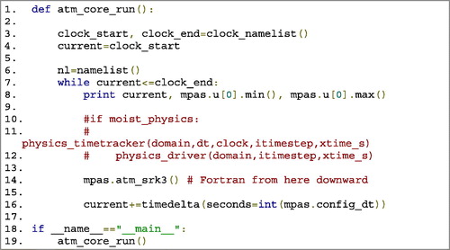
Operations involving date and time that are commonly encountered in controlling simulation flows are as simple as an arithmetic addition/subtraction and can be directly compared with each other. Parsing the namelist that specifies various parameters in the simulations can be easily achieved by the pre-existing package called F90Nml. The entire MPAS-A dynamical core written in Fortran can be compiled with the generic F2Py utility and become accessible in the Python code shown above.

Appendix B

Divergence under the Voronoi mesh

Under the mesh of Voronoi grids, the divergence at the centre of any given cell is calculated as follows: $$\nabla \cdot \mathbf{V}=\frac{1}{A}\sum _{n_{e_i}}{d}_{e_i}\mathbf{V}\cdot {\mathbf{n}}_{e_i},$$ where $\mathbf{V}$ is the wind vector, A is the area of the Voronoi cell, $d_{e_i}$ is the length of the ith edge of a cell and ${\mathbf{n}}_{e_i}$ is the unit vector in the normal direction of the ith edge. When written in Fortran 90, the above divergence calculation in the MPAS-A dynamic core is as follows:

where dvEdge is the distance of a cell edge. As the divergence is a linear function of the wind variable, the corresponding calculation of divergence in the TL model is the same as that in the MPAS-A model:

 

 

 

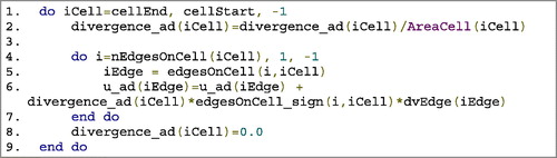
The corresponding calculation of this part in the adjoint model is as follows:

References

- Carrier, M. J., Zou, X. and Lapenta, W. M. 2008. Comparing the vertical structures of weighting functions and adjoint sensitivity of radiance and verifying mesoscale forecasts using AIRS radiance observations. Monthly Weather Rev. 136, 1327–1348. doi:10.1175/2007MWR2057.1
- Courtier, P., Derber, J., Errico, R., Louis, J. F. J.-F. and Vukicevic, T. 1993. Review of the use of adjoint, variational methods, and Kalman filters in meteorology. Tellus A 45, 342–357. doi:10.3402/tellusa.v45i5.14898
- Courtier, P. and Talagrand, O. 1990. Variational assimilation of meteorological observations with the direct and adjoint shallow-water equations. Tellus A 42, 531–549. doi:10.3402/tellusa.v42i5.11896
- Courtier, P., Thépaut, J. N. and Hollingsworth, A. 1994. A strategy for operational implementation of 4D‐Var, using an incremental approach. Q. J. Royal Meteorol. Soc. 120, 1367–1387. doi:10.1002/qj.49712051912
- Errico, R. M. 1997. What is an adjoint model? Bull. Am. Meteorol. Soc. 78, 2577–2592. doi:10.1175/1520-0477(1997)078<2577:WIAAM>2.0.CO;2
- Errico, R. M. and Vukicevic, T. 1992. Sensitivity analysis using an adjoint of the PSU-NCAR mesoseale model. Monthly Weather Rev. 120, 1644–1660. doi:10.1175/1520-0493(1992)120<1644:SAUAAO>2.0.CO;2
- Giering, R. and Kaminski, T. 2003. Applying TAF to generate efficient derivative code of Fortran 77‐95 programs. Proc. Appl. Math. Mech. 2, 54–57. doi:10.1002/pamm.200310014
- Hagos, S., Leung, R., Rauscher, S. A. and Ringler, T. 2013. Error characteristics of two grid refinement approaches in aquaplanet simulations: MPAS-A and WRF. Monthly Weather Rev. 141, 3022–3036. doi:10.1175/MWR-D-12-00338.1
- Jablonowski, C. and Williamson, D. L. 2006a. A Baroclinic Wave Test Case for Dynamical Cores of General Circulation Models: Model Intercomparisons. NCAR Technical Note (NCAR/TN–469 + STR). University Corporation for Atmospheric Research, Boulder, CO, USA.
- Jablonowski, C. and Williamson, D. L. 2006b. A baroclinic instability test case for atmospheric model dynamical cores. Q. J. Royal Meteorol. Soc. 132, 2943–2975. doi:10.1256/qj.06.12
- Le Dimet, F.-X. and Talagrand, O. 1986. Variational algorithms for analysis and assimilation of meteorological observations: theoretical aspects. Tellus A 38, 97–110. doi:10.3402/tellusa.v38i2.11706
- Lin, J. W.-B. 2012. Why Python is the next wave in earth sciences computing. Bull. Am. Meteorol. Soc. 93, 1823–1824. doi:10.1175/BAMS-D-12-00148.1
- Lutz, M. 2013. Learning Python: Powerful Object-Oriented Programming. 5th ed. O'Reilly Media, Inc. Newton, MA, USA.
- Park, S.-H., Skamarock, W. C., Klemp, J. B., Fowler, L. D. and Duda, M. G. 2013. Evaluation of global atmospheric solvers using extensions of the Jablonowski and Williamson baroclinic wave test case. Monthly Weather Rev. 141, 3116–3129. doi:10.1175/MWR-D-12-00096.1
- Peterson, P. 2009. F2PY: a tool for connecting Fortran and Python programs. Int. J. Comput. Sci. Eng.. 4, 296–305.
- Rabier, F., Courtier, P. and Talagrand, O. 1992. An application of adjoint models to sensitivity analysis. Beitr. Phys. Atmos. 65, 177–192.
- Rabier, F., Klinker, E., Courtier, P. and Hollingsworth, A. 1996. Sensitivity of forecast errors to initial conditions. Q. J. Royal Meteorol. Soc. 122, 121–150. doi:10.1002/qj.49712252906
- Rauscher, S. A. and Ringler, T. D. 2014. Impact of variable-resolution meshes on midlatitude baroclinic eddies using CAM-MPAS-A. Monthly Weather Rev. 142, 4256–4268. doi:10.1175/MWR-D-13-00366.1
- Ringler, T., Ju, L. and Gunzburger, M. 2008. A multiresolution method for climate system modeling: application of spherical centroidal Voronoi tessellations. Ocean Dyn. 58, 475–498. doi:10.1007/s10236-008-0157-2
- Satoh, M., Matsuno, T., Tomita, H., Miura, J., Nasuno, T. and co-authors. 2008. Nonhydrostatic icosahedral atmospheric model (NICAM) for global cloud resolving simulations. Comput. Phys. 227, 3486–3514. doi:10.1016/j.jcp.2007.02.006
- Skamarock, W. C. and Klemp, J. B. 2008. A time-split nonhydrostatic atmospheric model for weather research and forecasting applications. Comput. Phys. 227, 3465–3485. doi:10.1016/j.jcp.2007.01.037
- Skamarock, W. C., Klemp, J. B., Duda, M. G., Fowler, L. D., Park, S.-H. and co-authors. 2012. A multiscale nonhydrostatic atmospheric model using centroidal Voronoi tesselations and C-grid staggering. Monthly Weather Rev. 140, 3090–3105. doi:10.1175/MWR-D-11-00215.1
- Xiao, Q., Kuo, Y.-H., Ma, Z., Huang, W., Huang, X.-Y. and co-authors. 2008. Application of an adiabatic WRF adjoint to the investigation of the May 2004 McMurdo, Antarctica, severe wind event. Monthly Weather Rev. 136, 3696–3713. doi:10.1175/2008MWR2235.1
- Zou, X., Barcilon, A., Navon, I. M., Whitaker, J. and Cacuci, D. G. 1993. An adjoint sensitivity study of blocking in a two-layer isentropic model. Monthly Weather Rev. 121, 2833–2857. doi:10.1175/1520-0493(1993)121<2833:AASSOB>2.0.CO;2
- Zou, X. and Kuo, Y. H. 1996. Rainfall assimilation through an optimal control of initial and boundary conditions in a limited-area mesoscale model. Monthly Weather Rev. 124, 2859–2882. doi:10.1175/1520-0493(1996)124<2859:RATAOC>2.0.CO;2
- Zou, X., Kuo, Y. H. and Guo, Y. R. 1995. Assimilation of atmospheric radio refractivity using a nonhydrostatic adjoint model. Monthly Weather Rev. 123, 2229–2250. doi:10.1175/1520-0493(1995)123<2229:AOARRU>2.0.CO;2
- Zou, X., Vandenberghe, F., Pondeca, M. and Kuo, Y.-H. 1997. Introduction to adjoint techniques and the MM5 adjoint modeling system (No. NCAR/TN-435 + STR). University Corporation for Atmospheric Research..