Accounting for observation uncertainty and bias due to unresolved scales with the Schmidt-Kalman filter

Abstract

Data assimilation combines observations with numerical model data, to provide a best estimate of a real system. Errors due to unresolved scales arise when there is a spatio-temporal scale mismatch between the processes resolved by the observations and model. We present theory on error, uncertainty and bias due to unresolved scales for situations where observations contain information on smaller scales than can be represented by the numerical model. The Schmidt-Kalman filter, which accounts for the uncertainties in the unrepresented processes, is investigated and compared with an optimal Kalman filter that treats all scales, and a suboptimal Kalman filter that accounts for the large-scales only. The equation governing true analysis uncertainty is reformulated to include representation uncertainty for each filter. We apply the filters to a random walk model with one variable for large-scale processes and one variable for small-scale processes. Our new results show that the Schmidt-Kalman filter has the largest benefit over a suboptimal filter in regimes of high representation uncertainty and low instrument uncertainty but performs worse than the optimal filter. Furthermore, we review existing theory showing that errors due to unresolved scales often result in representation error bias. We derive a novel bias-correcting form of the Schmidt-Kalman filter and apply it to the random walk model with biased observations. We show that the bias-correcting Schmidt-Kalman filter successfully compensates for representation error biases. Indeed, it is more important to treat an observation bias than an unbiased error due to unresolved scales.

Keywords:

• data assimilation
• observation uncertainty
• error due to unresolved scales
• observation bias
• Schmidt-Kalman filter

1. Introduction

In atmospheric data assimilation, observations are combined with numerical model data, weighted by their respective error statistics, to provide a best estimate of the current atmospheric state, known as the analysis. This is achieved through comparison of observations with the numerical model equivalent of those observations. The errors associated with the observation-model comparison are the instrument error and representation error (Janjić et al., 2018). The representation error consists of the pre-processing error, the observation operator error and the error due to unresolved scales that occurs when there is a mismatch between the numerical model resolution and the scales resolved by the observation. The error due to unresolved scales depends on the observation footprint, which could be smaller or larger than the model grid, depending on the observation type and choice of model. For models which contain information on scales smaller than those observed, the standard approach to account for scale-mismatch would be to average the model state over the observation area (Janjić et al., 2018). However, for the purposes of this paper, we focus only on situations where the observation information content includes smaller scales than can be resolved by the model. In order to obtain the best analysis from these observations the representation error must be treated correctly by the data assimilation system.

Methods of accounting for uncertainty due to unresolved scales include, for example, prediction through ensemble statistics (Karspeck, 2016; Satterfield et al., 2017) and the use of a stochastic superparameterization (Grooms et al., 2014). In this manuscript we will consider two approaches: the standard approach where the uncertainty due to unresolved scales is included in the observation error covariance matrix (e.g. Hodyss and Satterfield, 2016; Fielding and Stiller, 2019) and an alternative approach where unresolved processes are considered in state space and hence accounted for through the state error covariance (Janjić and Cohn, 2006).

Compensating for representation error through the standard approach involves using an observation error covariance matrix that takes into account both the instrument and representation uncertainty. This can then be used within a standard variational or sequential data assimilation scheme. Estimates of the observation uncertainty may be obtained using a statistical method, to estimate the entire observation error covariance matrix (e.g. Desroziers et al., 2005; Stewart et al., 2014; Waller et al., 2016a, 2016b; Cordoba et al., 2017). Alternatively each component of the representation error statistics can be estimated separately and then combined with the instrument error covariance. For example the error due to unresolved scales may be approximated using high resolution observations (Oke and Sakov, 2008) or high resolution model data (Daley, 1993; Liu and Rabier, 2002; Waller et al., 2014; Schutgens et al., 2016).

The Schmidt-Kalman filter (SKF) (Schmidt, 1966) is an example of a filter which uses the statistics of the unresolved processes in state space, without ever evaluating the unresolved state itself, to compensate for the error due to unresolved scales. This approach allows for consideration of flow-dependent correlations between the resolved errors and the unresolved processes at the cost of additional assumptions, approximations and increased computational expense. Janjić and Cohn (2006) have shown that the SKF can produce positive results despite the approximations and assumptions required for implementation in a geophysical context. In this paper we provide new results that determine in which observation and model uncertainty regimes the SKF performs best. In addition we compare the SKF to two other Kalman filtering approaches.

The SKF is deemed a suboptimal filter as it does not minimise the mean-square-error of its estimated states (Janjić and Cohn, 2006). In contrast, the Kalman filter that treats all scales is deemed optimal (for linear models and Gaussian statistics) (Nichols, 2010). In practice, suboptimal filters that do not treat all scales are often used. The analysis error covariances propagated by suboptimal filters are not representative of the true error statistics due to omitted or incorrectly specified filter components. As such, the true analysis error equations have been derived to evaluate the performance of suboptimal filters (e.g. Brown and Sage, 1971; Asher and Reeves, 1975; Asher et al., 1976). In this article we reformulate previous theory on true analysis error equations to include representation error (section 4) and evaluate the performance of the SKF.

A further issue noted by Janjić and Cohn (2006) is the potential for the representation error to be biased. This is because the error due to unresolved scales is sequentially correlated in time and correlated with the state resolved by the model. Other authors have circumvented this bias by careful construction of their numerical model (Janjić and Cohn, 2006). However, in operational data assimilation, most observations are biased and the innovations need to be corrected or the bias accounted for within the assimilation (Dee, 2005). Bias correction can be incorporated into the data assimilation algorithm by augmenting the state vector with a bias term (Friedland, 1969; Jazwinski, 1970; Ignagni, 1981) which can be estimated along with the state variables. This method of bias correction is commonly used with variational data assimilation systems (e.g. Derber and Wu, 1998; Dee, 2004; Zhu et al., 2014; Eyre, 2016) but has also been applied with ensemble data assimilation systems (e.g. Fertig et al., 2009; Miyoshi et al., 2010; Aravéquia et al., 2011). To the best of our knowledge a bias correction scheme has yet to be implemented in conjunction with the SKF; in section 7 we introduce a bias-correcting SKF as a new method to compensate for biases due to unresolved scales.

In summary, the objective of this paper is to investigate under which model and observation error regimes the SKF is most effective. The theoretical aspects of representation error will be reviewed in section 2 with particular emphasis on the error due to unresolved scales. Section 3 details how the SKF can be used to account for error due to unresolved scales and introduces the optimal Kalman filter (OKF) and a reduced-state Kalman filter (RKF). In section 4 we state the standard true analysis error equation and reformulate it to include representation error for each filter.

To evaluate the performance of the SKF in a numerical example we use a Gaussian random walk model. The numerical experiment methodology and model formulation are described in section 5 and results are presented in section 6. Our results show that the SKF provides the largest improvement in performance compared with the RKF when there is large error variance due to unresolved scales and small instrument error variance. In section 7 we discuss observation bias correction schemes in sequential data assimilation and introduce a novel SKF with bias correction scheme. The methodology and model formulation for the numerical experiments with biased observations is discussed in section 8 and results are presented in section 9. Our results show the SKF with bias correction can simultaneously treat observation biases and compensate for the error due to unresolved scales. We summarise and draw conclusions from our results in section 10.

2. Theoretical framework

In this section we introduce a theoretical framework and the notation used in this paper. We begin by describing a numerical model (section 2.1) and observations (section 2.2). In data assimilation, the error statistics used in filters may not reflect the true uncertainties they are intended to model. To help distinguish between these two sets of statistics throughout this manuscript we will define any true error statistics with a tilde (∼). Error statistics used in or obtained from filter calculations will be referred to as perceived error statistics and have no tilde.

The mathematical framework used to examine the error due to unresolved scales in this manuscript is to estimate the projection of some state from a high, but finite dimensional real vector space, onto a lower dimensional subspace using observations and knowledge of the system dynamics, following a similar philosophy to Liu and Rabier (2002) and Waller et al. (2014). Our approach differs from that of Janjić and Cohn (2006) which begins from the standpoint of infinite dimensional function spaces.

2.1. Model configuration

In this section we introduce the perfect and forecast models. We assume that the phase-space for the large-scale dynamics is a subspace of the phase-space for the full high dimensional system. The complement of the subspace for the large-scales will correspond to the phase-space for the small-scale dynamics. The notation for the models will be in a partitioned form that separates the large and small scales. In particular, we denote the true, complete state at time t_k as ${(\begin{array}{cc}{\mathit{x}}^{l,t}& {\mathit{x}}^{s,t}\end{array})}_k^T\in {\mathbb{R}}^{N_t}$ such that ${\mathit{x}}^{l,t}\in {\mathrm{ℝ}}^{N_l}, {\mathit{x}}^{s,t}\in {\mathrm{ℝ}}^{N_s}$ and $N_t=N_l+N_s.$ Here, and throughout this paper, any component with a t-superscript indicates that it is a true variable. The l- and s-superscripts correspond to the large- and small-scale processes within the complete system dynamics. (We have deviated from the resolved/unresolved nomenclature of Janjic and Cohn 2006 for clarity, since the different filters used in our experiments resolve different scales).

An ideal linear model for the true state of a finite dimensional process can be expressed through the dynamical system (2.1) $${\left(\begin{array}{c}{\mathit{x}}^{l,t}\\ {\mathit{x}}^{s,t}\end{array}\right)}_k=\left(\begin{array}{cc}{\mathbf{M}}^{l,t}& {\mathbf{M}}^{ls,t}\\ {\mathbf{M}}^{sl,t}& {\mathbf{M}}^{s,t}\end{array}\right){\left(\begin{array}{c}{\mathit{x}}^{l,t}\\ {\mathit{x}}^{s,t}\end{array}\right)}_{k-1},$$(2.1) such that the matrix blocks ${\mathbf{M}}^{l,t}\in {\mathrm{ℝ}}^{N_l\times N_l}, {\mathbf{M}}^{ls,t}\in {\mathrm{ℝ}}^{N_l\times N_s}, {\mathbf{M}}^{s,t}\in {\mathrm{ℝ}}^{N_s\times N_s}$ and ${\mathbf{M}}^{sl,t}\in {\mathbb{R}}^{N_s\times N_l}.$ From a numerical modelling perspective, this partitioned description of the dynamics would be suited to a pseudospectral discretization (e.g. Fourier modes).

In numerical weather prediction (NWP), the true models that govern the evolution of the atmosphere are unknown and have to be approximated. For our approximation of the true dynamical system (2.1)(2.1) $${\left(\begin{array}{c}{\mathit{x}}^{l,t}\\ {\mathit{x}}^{s,t}\end{array}\right)}_k=\left(\begin{array}{cc}{\mathbf{M}}^{l,t}& {\mathbf{M}}^{ls,t}\\ {\mathbf{M}}^{sl,t}& {\mathbf{M}}^{s,t}\end{array}\right){\left(\begin{array}{c}{\mathit{x}}^{l,t}\\ {\mathit{x}}^{s,t}\end{array}\right)}_{k-1},$$(2.1) , we assume that any subgrid-scale parameterizations used to approximate the contribution from the small-scale processes to the large-scale state are contained within the large-scale model (Janjić and Cohn, 2006; Janjić et al., 2018). Hence, the model block ${\mathbf{M}}^{ls}={\mathbf{0}}_{N_l\times N_s}$ and our approximate dynamical model describing the complete system satisfies (2.2) $${\left(\begin{array}{c}{\mathit{x}}^{l,t}\\ {\mathit{x}}^{s,t}\end{array}\right)}_k=\left(\begin{array}{cc}{\mathbf{M}}^l& {\mathbf{0}}_{N_l\times N_s}\\ {\mathbf{M}}^{sl}& {\mathbf{M}}^s\end{array}\right){\left(\begin{array}{c}{\mathit{x}}^{l,t}\\ {\mathit{x}}^{s,t}\end{array}\right)}_{k-1}-{\left(\begin{array}{c}{\mathit{\eta }}^l\\ {\mathit{\eta }}^s\end{array}\right)}_k.$$(2.2)

In (2.2)(2.2) $${\left(\begin{array}{c}{\mathit{x}}^{l,t}\\ {\mathit{x}}^{s,t}\end{array}\right)}_k=\left(\begin{array}{cc}{\mathbf{M}}^l& {\mathbf{0}}_{N_l\times N_s}\\ {\mathbf{M}}^{sl}& {\mathbf{M}}^s\end{array}\right){\left(\begin{array}{c}{\mathit{x}}^{l,t}\\ {\mathit{x}}^{s,t}\end{array}\right)}_{k-1}-{\left(\begin{array}{c}{\mathit{\eta }}^l\\ {\mathit{\eta }}^s\end{array}\right)}_k.$$(2.2) each model block has the same dimensions as its true model counterpart. The large- and small-scale model errors are given by ${\mathit{\eta }}^l\in {\mathrm{ℝ}}^{N_l}$ and ${\mathit{\eta }}^s\in {\mathrm{ℝ}}^{N_s}$ respectively. Model errors are assumed to be random and unbiased with covariance given by (2.3) $$\tilde{\mathbf{Q}}=\left(\begin{array}{cc}{\tilde{\mathbf{Q}}}^{ll}& {\tilde{\mathbf{Q}}}^{ls}\\ {\tilde{\mathbf{Q}}}^{sl}& {\tilde{\mathbf{Q}}}^{ss}\end{array}\right).$$(2.3)

Here, using $〈·〉$ to indicate the mathematical expectation over the corresponding error distribution, the matrices ${\tilde{\mathbf{Q}}}^{ll}\equiv 〈{\mathit{\eta }}^l{\left({\mathit{\eta }}^l\right)}^T〉\in {\mathrm{ℝ}}^{N_l\times N_l}, {\tilde{\mathbf{Q}}}^{ss}\equiv 〈{\mathit{\eta }}^s{\left({\mathit{\eta }}^s\right)}^T〉\in {\mathrm{ℝ}}^{N_s\times N_s}$ and ${\tilde{\mathbf{Q}}}^{ls}\equiv 〈{\mathit{\eta }}^l{\left({\mathit{\eta }}^s\right)}^T〉\in {\mathrm{ℝ}}^{N_l\times N_s}$ (with ${\tilde{\mathbf{Q}}}^{ls}={({\tilde{\mathbf{Q}}}^{sl})}^T$) are the true model error covariances of the large-scale, the small-scale and cross-covariances between the large- and small-scale, respectively. We note that for the purposes of this work, the model error distribution is assumed to be stationary, so that $\tilde{\mathbf{Q}}$ is not a function of time.

Analogously, the complete forecast state ${(\begin{array}{cc}{\mathit{x}}^{l,f}& {\mathit{x}}^{s,f}\end{array})}^T\in {\mathbb{R}}^{N_t}$ satisfies (2.4) $${\left(\begin{array}{c}{\mathit{x}}^{l,f}\\ {\mathit{x}}^{s,f}\end{array}\right)}_k=\left(\begin{array}{cc}{\mathbf{M}}^l& {\mathbf{0}}_{N_l\times N_s}\\ {\mathbf{M}}^{sl}& {\mathbf{M}}^s\end{array}\right){\left(\begin{array}{c}{\mathit{x}}^{l,f}\\ {\mathit{x}}^{s,f}\end{array}\right)}_{k-1}.$$(2.4)

The forecast errors can then be defined as (2.5) $${\left(\begin{array}{c}{\mathbf{e}}^{l,f}\\ {\mathbf{e}}^{s,f}\end{array}\right)}_k\equiv {\left(\begin{array}{c}{\mathit{x}}^{l,f}\\ {\mathit{x}}^{s,f}\end{array}\right)}_k-{\left(\begin{array}{c}{\mathit{x}}^{l,t}\\ {\mathit{x}}^{s,t}\end{array}\right)}_k=\left(\begin{array}{cc}{\mathbf{M}}^l& {\mathbf{0}}_{N_l\times N_s}\\ {\mathbf{M}}^{sl}& {\mathbf{M}}^s\end{array}\right){\left(\begin{array}{c}{\mathbf{e}}^{l,f}\\ {\mathbf{e}}^{s,f}\end{array}\right)}_{k-1}+{\left(\begin{array}{c}{\mathit{\eta }}^l\\ {\mathit{\eta }}^s\end{array}\right)}_k,$$(2.5) where ${\mathbf{e}}^{l,f}\in {\mathbb{R}}^{N_l}$ and ${\mathbf{e}}^{s,f}\in {\mathbb{R}}^{N_s}$ are the large- and small-scale forecast errors respectively. The true forecast error covariance is denoted (2.6) $${\tilde{\mathbf{P}}}_k^f={\left(\begin{array}{cc}{\tilde{\mathbf{P}}}^{ll,f}& {\tilde{\mathbf{P}}}^{ls,f}\\ {\tilde{\mathbf{P}}}^{sl,f}& {\tilde{\mathbf{P}}}^{ss,f}\end{array}\right)}_k.$$(2.6)

Here, ${\tilde{\mathbf{P}}}_k^{ll,f}\equiv 〈{\mathbf{e}}_k^{l,f}{\left({\mathbf{e}}_k^{l,f}\right)}^T〉\in {\mathrm{ℝ}}^{N_l\times N_l}, {\tilde{\mathbf{P}}}_k^{ss,f}\equiv 〈{\mathbf{e}}_k^{s,f}{\left({\mathbf{e}}_k^{s,f}\right)}^T〉\in {\mathrm{ℝ}}^{N_s\times N_s}$ and ${\tilde{\mathbf{P}}}_k^{ls,f}\equiv 〈{\mathbf{e}}_k^{l,f}{({\mathbf{e}}_k^{s,f})}^T〉\in {\mathbb{R}}^{N_l\times N_s}$ (with ${\tilde{\mathbf{P}}}^{ls,f}={({\tilde{\mathbf{P}}}^{sl,f})}^T$) are the true forecast error covariances of the large-scale, the small-scale and cross-covariances between the large- and small-scale, respectively.

This formulation of the complete finite-dimensional dynamics allows us to consider several filters with different approaches to the treatment of large- and small-scales. Moreover, we can consider the interactions between scales and the effect they have on the modelling of observations.

2.2. Observations and their uncertainties

In this section we express the equations relating the observations, ${\mathit{y}}_k\in {\mathbb{R}}^p,$ to the model state in a partitioned form and describe their uncertainties. For the rest of this section, we assume that the model state and observations are valid at the same time, and drop the time subscript, k. At time t_k, the observations are related to the true model state as (2.7) $$\mathit{y}=\left(\begin{array}{cc}{\mathbf{H}}^{l,t}& {\mathbf{H}}^{s,t}\end{array}\right)\left(\begin{array}{c}{\mathit{x}}^{l,t}\\ {\mathit{x}}^{s,t}\end{array}\right)+\mathit{ϵ},$$(2.7) where $\mathit{ϵ}\in {\mathrm{ℝ}}^p$ is the instrument error, assumed to be random and unbiased with covariance ${\tilde{\mathbf{R}}}^I=〈\mathit{ϵ}{\mathit{ϵ}}^T〉\in {\mathrm{ℝ}}^{p\times p}$ and ${\mathbf{H}}^{l,t}\in {\mathbb{R}}^{p\times N_l}$ and ${\mathbf{H}}^{s,t}\in {\mathbb{R}}^{p\times N_s}$ are the true linear observation operators which map the large- and small-scale states into observation space respectively. The observation operator $(\begin{array}{cc}{\mathbf{H}}^{l,t}& {\mathbf{H}}^{s,t}\end{array})$ is the (linear) finite-dimensional counterpart to the continuum observation operator of Janjić and Cohn (2006). We will not consider nonlinear observation operators in the remainder of this paper.

Throughout this paper, we assume that there is no pre-processing error. Hence, we will be concerned with the two cases described in sections 2.2.1 (all scales analysed) and 2.2.2 (large scales analysed) below. Case 1 shows the form of the representation error for filters that resolve all scales and is pertinent to the theoretical optimal Kalman filter discussed in section 3.2. Case 2 shows the form of the representation error for filters typically used in operational practice and is pertinent to the reduced-state Kalman filter and the Schmidt-Kalman filter discussed in sections 3.3 and 3.4 respectively.

2.2.1. Case 1: All scales analysed

In this case we assume that both the large- and small-scale states are estimated. The total observation error (observation departure from the true state), ${\mathbf{e}}^o,$ can be expressed as (2.8) $${\mathbf{e}}^o=\mathit{y}-\left(\begin{array}{cc}{\mathbf{H}}^l& {\mathbf{H}}^s\end{array}\right)\left(\begin{array}{c}{\mathit{x}}^{l,t}\\ {\mathit{x}}^{s,t}\end{array}\right),$$(2.8) where ${\mathbf{H}}^l\in {\mathbb{R}}^{p\times N_l}$ and ${\mathbf{H}}^s\in {\mathbb{R}}^{p\times N_s}$ are the blocks of the observation operator used by the filter, acting on the large- and small-scale state components, respectively. Using (2.7)(2.7) $$\mathit{y}=\left(\begin{array}{cc}{\mathbf{H}}^{l,t}& {\mathbf{H}}^{s,t}\end{array}\right)\left(\begin{array}{c}{\mathit{x}}^{l,t}\\ {\mathit{x}}^{s,t}\end{array}\right)+\mathit{ϵ},$$(2.7) , we rewrite ${\mathbf{e}}^o$ as (2.9) $$\begin{array}{c}{\mathbf{e}}^o=\left(\begin{array}{cc}{\mathbf{H}}^{l,t}& {\mathbf{H}}^{s,t}\end{array}\right)\left(\begin{array}{c}{\mathit{x}}^{l,t}\\ {\mathit{x}}^{s,t}\end{array}\right)+\mathit{ϵ}-\left(\begin{array}{cc}{\mathbf{H}}^l& {\mathbf{H}}^s\end{array}\right)\left(\begin{array}{c}{\mathit{x}}^{l,t}\\ {\mathit{x}}^{s,t}\end{array}\right),\\ =({\mathbf{H}}^{l,t}-{\mathbf{H}}^l){\mathit{x}}^{l,t}+({\mathbf{H}}^{s,t}-{\mathbf{H}}^s){\mathit{x}}^{s,t}+\mathit{ϵ},\\ ={\mathit{\gamma }}^l+{\mathit{\gamma }}^s+\mathit{ϵ},\end{array}$$(2.9) where ${\mathit{\gamma }}^l\equiv ({\mathbf{H}}^{l,t}-{\mathbf{H}}^l){\mathit{x}}^{l,t}$ is the large-scale observation operator error and ${\mathit{\gamma }}^s\equiv ({\mathbf{H}}^{s,t}-{\mathbf{H}}^s){\mathit{x}}^{s,t}$ is the small-scale observation operator error. Thus, the representation error for this case consists solely of observation operator error, ${\mathit{\gamma }}^l+{\mathit{\gamma }}^s.$ The observation operator errors, ${\mathit{\gamma }}^l$ and ${\mathit{\gamma }}^s,$ will each be assumed to be unbiased, so that in this case, the representation error is also unbiased. The representation error covariance for this case will be denoted by ${\tilde{\mathbf{R}}}^G=〈({\mathit{\gamma }}^l+{\mathit{\gamma }}^s){({\mathit{\gamma }}^l+{\mathit{\gamma }}^s)}^T〉\in {\mathrm{ℝ}}^{p\times p}.$ The total observation error covariance is given by $\tilde{\mathbf{R}}={\tilde{\mathbf{R}}}^I+{\tilde{\mathbf{R}}}^G,$ where we have assumed that the representation error and instrument error are mutually uncorrelated.

2.2.2. Case 2: Large scales analysed

In this case, we assume that only the large-scale state is estimated such that (2.10) $${\mathbf{e}}^o=\mathit{y}-{\mathbf{H}}^l{\mathit{x}}^{l,t},$$(2.10) where the observation operator used consists only of the block acting on the large-scales. The decomposition of ${\mathbf{e}}^o$ can be obtained by setting ${\mathbf{H}}^s={\mathbf{0}}_{p\times N_s}$ in (2.9)(2.9) $$\begin{array}{c}{\mathbf{e}}^o=\left(\begin{array}{cc}{\mathbf{H}}^{l,t}& {\mathbf{H}}^{s,t}\end{array}\right)\left(\begin{array}{c}{\mathit{x}}^{l,t}\\ {\mathit{x}}^{s,t}\end{array}\right)+\mathit{ϵ}-\left(\begin{array}{cc}{\mathbf{H}}^l& {\mathbf{H}}^s\end{array}\right)\left(\begin{array}{c}{\mathit{x}}^{l,t}\\ {\mathit{x}}^{s,t}\end{array}\right),\\ =({\mathbf{H}}^{l,t}-{\mathbf{H}}^l){\mathit{x}}^{l,t}+({\mathbf{H}}^{s,t}-{\mathbf{H}}^s){\mathit{x}}^{s,t}+\mathit{ϵ},\\ ={\mathit{\gamma }}^l+{\mathit{\gamma }}^s+\mathit{ϵ},\end{array}$$(2.9) : (2.11) $${\mathbf{e}}^o={\mathit{\gamma }}^l+{\mathbf{H}}^{s,t}{\mathit{x}}^{s,t}+\mathit{ϵ}.$$(2.11)

The filter observation operator does not act on the small scales, so the term ${\mathit{\gamma }}^s$ is replaced by ${\mathbf{H}}^{s,t}{\mathit{x}}^{s,t},$ the error due to unresolved scales. The representation error for Case 2 is thus ${\mathit{\gamma }}^l+{\mathbf{H}}^{s,t}{\mathit{x}}^{s,t}$ with covariance ${\tilde{\mathbf{R}}}^H=〈({\mathit{\gamma }}^l+{\mathbf{H}}^{s,t}{\mathit{x}}^{s,t}){({\mathit{\gamma }}^l+{\mathbf{H}}^{s,t}{\mathit{x}}^{s,t})}^T〉\in {\mathrm{ℝ}}^{p\times p}.$ Equations (2.10)(2.10) $${\mathbf{e}}^o=\mathit{y}-{\mathbf{H}}^l{\mathit{x}}^{l,t},$$(2.10) and (2.11)(2.11) $${\mathbf{e}}^o={\mathit{\gamma }}^l+{\mathbf{H}}^{s,t}{\mathit{x}}^{s,t}+\mathit{ϵ}.$$(2.11) are analogous to equation (1) in Janjić et al. (2018) with the pre-processing error omitted. The complete observation error covariance for Case 2 is given by $\tilde{\mathbf{R}}={\tilde{\mathbf{R}}}^I+{\tilde{\mathbf{R}}}^H,$ where we have assumed that the representation error and instrument error are mutually uncorrelated. As in Case 1, ${\mathit{\gamma }}^l$ is assumed to be unbiased. However, we will see in section 2.3 that the expected value of ${\mathbf{H}}^{s,t}{\mathit{x}}^{s,t}$ is likely to be non-zero.

2.3. Bias due to unresolved scales

Analysing only the large-scales will result in an error due to unresolved scales (section 2.2.2) that is sequentially correlated in time and correlated with the resolved state, leading to a potential bias (Janjić and Cohn, 2006). Assuming that the large-scale observation operator is unbiased, taking the expectation of the error due to unresolved scales, (2.11)(2.11) $${\mathbf{e}}^o={\mathit{\gamma }}^l+{\mathbf{H}}^{s,t}{\mathit{x}}^{s,t}+\mathit{ϵ}.$$(2.11) , (and reintroducing the time subscript k) results in (2.12) $$〈{\mathbf{e}}^o〉=〈{\mathbf{H}}^{s,t}{\mathit{x}}_k^{s,t}〉,$$(2.12) where $〈·〉$ denotes the mathematical expectation over the distribution of representation errors at time k. Using dynamical system (2.1)(2.1) $${\left(\begin{array}{c}{\mathit{x}}^{l,t}\\ {\mathit{x}}^{s,t}\end{array}\right)}_k=\left(\begin{array}{cc}{\mathbf{M}}^{l,t}& {\mathbf{M}}^{ls,t}\\ {\mathbf{M}}^{sl,t}& {\mathbf{M}}^{s,t}\end{array}\right){\left(\begin{array}{c}{\mathit{x}}^{l,t}\\ {\mathit{x}}^{s,t}\end{array}\right)}_{k-1},$$(2.1) , repeated substitution for the equation governing ${\mathit{x}}^{s,t}$ into the expected error due to unresolved scales yields (2.13) $$〈{\mathbf{H}}^{s,t}{\mathit{x}}_k^{s,t}〉=〈{\mathbf{H}}^{s,t}(\underset{¯}{{\mathbf{M}}^{sl,t}{\mathit{x}}_{k-1}^{l,t}}+{\mathbf{M}}^{s,t}(\underset{¯}{{\mathbf{M}}^{sl,t}{\mathit{x}}_{k-2}^{l,t}}+{\mathbf{M}}^{s,t}(\dots (\underset{¯}{{\mathbf{M}}^{sl,t}{\mathit{x}}_0^{l,t}}+{\mathbf{M}}^{s,t}\left({\mathit{x}}_0^{s,t}\right))\dots )\left)\right)〉,$$(2.13)

Here the underlined terms represent the contribution from the large scales. For many non-trivial models, these terms will not be identically zero, and potentially introduce a bias even if the initial value for the small-scale state is zero, ${\mathit{x}}_0^{s,t}=\mathbf{0}.$ For example, Janjić and Cohn (2006) solved a model of non-divergent linear advection on a sphere using a truncated expansion in spherical harmonics. Introducing a shear flow results in a dynamical system where the unresolved small-scales do not directly influence the resolved large-scales, but the large-scales influence the small-scales. This yields an error and bias due to unresolved scales. Janjić and Cohn (2006) were able to mitigate the bias using specific initial conditions. However, this experimental freedom would not be available in less-idealized situations. Therefore, when accounting for the unresolved scales in data assimilation we must also determine and treat any bias arising. In the new results in sections 5-6 below, we carefully construct our model to avoid bias due to unresolved scales. However, we revisit this problem in sections 7-9 where we use filters with bias-correction schemes.

3. Sequential linear filters and representation uncertainty

In this section we describe the general linear filtering framework that we use for data assimilation in our theoretical investigations and numerical experiments. We consider three filters in more detail: an optimal Kalman filter (OKF) that takes account of all scales; a reduced-state Kalman filter (RKF) that disregards the small-scales; and the Schmidt-Kalman filter (SKF) that provides analyses of the large-scale state through consideration of both the large- and small-scale uncertainties.

3.1. A linear filter

A linear filter algorithm can be divided into analysis update and model prediction steps. The general form of the analysis update at time t_k, is given by (3.1) $${\mathit{x}}_k^a={\mathit{x}}_k^f+{\mathbf{K}}_k{\mathbf{d}}_k^{o,f},$$(3.1) where ${\mathit{x}}_k^a$ is the analysis (state estimate), ${\mathit{x}}_k^f$ is the forecast state, ${\mathbf{K}}_k$ is the gain matrix and ${\mathbf{d}}_k^{o,f}={\mathit{y}}_k-{\mathbf{H}}_k{\mathit{x}}_k^f$ is the innovation, defined as the observation-minus-forecast departure. In this general setting we have not defined the dimensions of the vectors and matrices in (3.1)(3.1) $${\mathit{x}}_k^a={\mathit{x}}_k^f+{\mathbf{K}}_k{\mathbf{d}}_k^{o,f},$$(3.1) , as this will depend on the specific choice of filter. For example, the state x in equation (3.1)(3.1) $${\mathit{x}}_k^a={\mathit{x}}_k^f+{\mathbf{K}}_k{\mathbf{d}}_k^{o,f},$$(3.1) could be either the complete state ${(\begin{array}{cc}{\mathit{x}}^l& {\mathit{x}}^s\end{array})}^T$ or just the large-scale state ${\mathit{x}}^l.$ There are various approaches to determine the gain matrix which will be discussed in sections 3.2, 3.3 and 3.4.

The perceived analysis error covariance update calcluated by the filter at time t_k is given by (3.2) $${\mathbf{P}}_k^a=\left(\mathbf{I}-{\mathbf{K}}_k{\mathbf{H}}_k\right){\mathbf{P}}_k^f,$$(3.2) where I is the identity matrix, ${\mathbf{H}}_k$ is the observation operator and ${\mathbf{P}}_k^f$ is the perceived forecast error covariance. Equation (3.2)(3.2) $${\mathbf{P}}_k^a=\left(\mathbf{I}-{\mathbf{K}}_k{\mathbf{H}}_k\right){\mathbf{P}}_k^f,$$(3.2) is known as the short form of the analysis error covariance update. This equation only provides the correct estimate of the analysis error covariance if the background and observation error statistics used in the filter reflect the true error statistics. The use of a suboptimal gain and the short form update equation (3.2)(3.2) $${\mathbf{P}}_k^a=\left(\mathbf{I}-{\mathbf{K}}_k{\mathbf{H}}_k\right){\mathbf{P}}_k^f,$$(3.2) will result in the filter producing incorrect error statistics. The true error statistics will be derived in section 4.

For the model prediction step, the forecast state at time $t_{k+1}$ is evolved from the analysis at the previous time-step and is given by (3.3) $${\mathit{x}}_{k+1}^f=\mathbf{M}{\mathit{x}}_k^a,$$(3.3) where M is a linear model. A model error term is not included in the forecast state update as linear filters estimate the mean state and we have assumed that the model error is unbiased. However, the error in the model M is accounted for in the forecast error covariance update given by (3.4) $${\mathbf{P}}_{k+1}^f=\mathbf{M}{\mathbf{P}}_k^a{\mathbf{M}}^T+\mathbf{Q},$$(3.4) which will be discussed further in section 4. We note that (3.4)(3.4) $${\mathbf{P}}_{k+1}^f=\mathbf{M}{\mathbf{P}}_k^a{\mathbf{M}}^T+\mathbf{Q},$$(3.4) will only produce correct error statistics when ${\mathbf{P}}_k^a$ and Q are equal to their true statistics counterparts.

Equations (3.1)(3.1) $${\mathit{x}}_k^a={\mathit{x}}_k^f+{\mathbf{K}}_k{\mathbf{d}}_k^{o,f},$$(3.1) –(3.4)(3.4) $${\mathbf{P}}_{k+1}^f=\mathbf{M}{\mathbf{P}}_k^a{\mathbf{M}}^T+\mathbf{Q},$$(3.4) form the core components of the linear filter algorithm. In the following sections we discuss three linear filters, each based on the Kalman filter (Kalman, 1960), that we will use in this paper. Table 1 summarizes the key vectors and matrices used in these three Kalman filters.

Table 1. The filter matrices and vectors for the Optimal Kalman filter (OKF), reduced-state Kalman filter (RKF) and Schmidt Kalman filter (SKF). The equations for the three filters are obtained through substituting these terms into (3.1) - (3.4). As discussed in section 3.4, we note that while the SKF uses ${\mathbf{H}}^{\mathbf{l}}$ in the innovation only, the complete observation operator is used in the calculation of ${\mathbf{K}}^{\mathbf{l}}$ and $\mathbf{D}.$

	OKF	RKF	SKF
State: x	$\left(\begin{array}{c}{\mathit{x}}^l\\ {\mathit{x}}^s\end{array}\right)\in {\mathbb{R}}^{N_t}$	${\mathit{x}}^l\in {\mathbb{R}}^{N_l}$	${\mathit{x}}^l\in {\mathbb{R}}^{N_l}$
State error covariance: P	$\left(\begin{array}{cc}{\mathbf{P}}^{ll}& {\mathbf{P}}^{ls}\\ {\mathbf{P}}^{sl}& {\mathbf{P}}^{ss}\end{array}\right)\in {\mathbb{R}}^{N_t\times N_t}$	${\mathbf{P}}^{ll}\in {\mathbb{R}}^{N_l\times N_l}$	$\left(\begin{array}{cc}{\mathbf{P}}^{ll}& {\mathbf{P}}^{ls}\\ {\mathbf{P}}^{sl}& {\mathbf{C}}^s\end{array}\right)\in {\mathbb{R}}^{N_t\times N_t}$
Observation operator: H	$\left(\begin{array}{cc}{\mathbf{H}}^l& {\mathbf{H}}^s\end{array}\right)\in {\mathbb{R}}^{p\times N_t}$	${\mathbf{H}}^l\in {\mathbb{R}}^{p\times N_l}$	$\left(\begin{array}{cc}{\mathbf{H}}^l& {\mathbf{H}}^s\end{array}\right)\in {\mathbb{R}}^{p\times N_t}$
Observation Error Covariance: R	${\mathbf{R}}^I+{\mathbf{R}}^G$	${\mathbf{R}}^I+{\mathbf{R}}^H$	${\mathbf{R}}^I+{\mathbf{R}}^G$
Innovation: ${\mathbf{d}}^{o,f}$	$\mathit{y}-\left(\begin{array}{cc}{\mathbf{H}}^l& {\mathbf{H}}^s\end{array}\right)\left(\begin{array}{c}{\mathit{x}}^{l,f}\\ {\mathit{x}}^{s,f}\end{array}\right)$	$\mathit{y}-{\mathbf{H}}^l{\mathit{x}}^{l,f}$	$\mathit{y}-{\mathbf{H}}^l{\mathit{x}}^{l,f}$
Innovation covariance: D	$\left(\begin{array}{cc}{\mathbf{H}}^l& {\mathbf{H}}^s\end{array}\right)\left(\begin{array}{cc}{\mathbf{P}}^{ll,f}& {\mathbf{P}}^{ls,f}\\ {\mathbf{P}}^{sl,f}& {\mathbf{P}}^{ss,f}\end{array}\right)\left(\begin{array}{c}{\left({\mathbf{H}}^l\right)}^T\\ {\left({\mathbf{H}}^s\right)}^T\end{array}\right)+\mathbf{R}$	${\mathbf{H}}^l{\mathbf{P}}^{ll,f}{\left({\mathbf{H}}^l\right)}^T+\mathbf{R}$	$\left(\begin{array}{cc}{\mathbf{H}}^l& {\mathbf{H}}^s\end{array}\right)\left(\begin{array}{cc}{\mathbf{P}}^{ll,f}& {\mathbf{P}}^{ls,f}\\ {\mathbf{P}}^{sl,f}& {\mathbf{C}}^s\end{array}\right)\left(\begin{array}{c}{\left({\mathbf{H}}^l\right)}^T\\ {\left({\mathbf{H}}^s\right)}^T\end{array}\right)+\mathbf{R}$
Kalman gain: K	$\left(\begin{array}{c}{\mathbf{K}}^l\\ {\mathbf{K}}^s\end{array}\right)=\left(\begin{array}{cc}{\mathbf{P}}^{ll,f}& {\mathbf{P}}^{ls,f}\\ {\mathbf{P}}^{sl,f}& {\mathbf{P}}^{ss,f}\end{array}\right)\left(\begin{array}{c}{\left({\mathbf{H}}^l\right)}^T\\ {\left({\mathbf{H}}^s\right)}^T\end{array}\right){\mathbf{D}}^{-1}$	${\mathbf{K}}^l=\left({\mathbf{P}}^{ll,f}{\left({\mathbf{H}}^l\right)}^T\right){\mathbf{D}}^{-1}$	$\begin{array}{c}\text{State}\mathrm{ }\text{update}\hfill \\ {\mathbf{K}}^l=\left({\mathbf{P}}^{ll,f}{\left({\mathbf{H}}^l\right)}^T+{\mathbf{P}}^{ls,f}{\left({\mathbf{H}}^s\right)}^T\right){\mathbf{D}}^{-1}\hfill \\ \text{Covariance}\mathrm{ }\text{update}\hfill \\ \left(\begin{array}{c}{\mathbf{K}}^l\\ {\mathbf{K}}^s\end{array}\right)=\left(\begin{array}{c}\left({\mathbf{P}}^{ll,f}{\left({\mathbf{H}}^l\right)}^T+{\mathbf{P}}^{ls,f}{\left({\mathbf{H}}^s\right)}^T\right){\mathbf{D}}^{-1}\\ {\mathbf{0}}_{N_s\times p}\end{array}\right)\hfill \end{array}$
Forecast model: M	$\left(\begin{array}{cc}{\mathbf{M}}^l& {\mathbf{0}}_{N_l\times N_s}\\ {\mathbf{M}}^{sl}& {\mathbf{M}}^s\end{array}\right)\in {\mathbb{R}}^{N_t\times N_t}$	${\mathbf{M}}^l\in {\mathbb{R}}^{N_l\times N_l}$	$\begin{array}{c}\text{State}\mathrm{ }\text{update}\hfill \\ {\mathbf{M}}^l\in {\mathbb{R}}^{N_l\times N_l}\hfill \\ \text{Covariance}\mathrm{ }\text{update}\hfill \\ \left(\begin{array}{cc}{\mathbf{M}}^l& {\mathbf{0}}_{N_l\times N_s}\\ {\mathbf{M}}^{sl}& {\mathbf{M}}^s\end{array}\right)\in {\mathbb{R}}^{N_t\times N_t}\hfill \end{array}$
Model Error Covariance: Q	$\left(\begin{array}{cc}{\mathbf{Q}}^{ll}& {\mathbf{Q}}^{ls}\\ {\mathbf{Q}}^{sl}& {\mathbf{Q}}^{ss}\end{array}\right)\in {\mathbb{R}}^{N_t\times N_t}$	${\mathbf{Q}}^{ll}\in {\mathbb{R}}^{N_l\times N_l}$	$\left(\begin{array}{cc}{\mathbf{Q}}^{ll}& {\mathbf{Q}}^{ls}\\ {\mathbf{Q}}^{sl}& {\mathbf{Q}}^{ss}\end{array}\right)\in {\mathbb{R}}^{N_t\times N_t}$

3.2. The optimal kalman filter (OKF)

For the optimal Kalman filter (OKF), we assume that we are able to model the processes for all scales and know the correct error statistics for the initial state, observations and model. Therefore, the perceived error statistics for the OKF will be equivalent to the true error statistics. The OKF simultaneously updates the large- and small-scale states, ${\mathit{x}}^l\in {\mathbb{R}}^{N_l}$ and ${\mathit{x}}^s\in {\mathbb{R}}^{N_s},$ so that the analysis update takes the form (3.5) $$\left(\begin{array}{c}{\mathit{x}}^{l,a}\\ {\mathit{x}}^{s,a}\end{array}\right)=\left(\begin{array}{c}{\mathit{x}}^{l,f}\\ {\mathit{x}}^{s,f}\end{array}\right)+\left(\begin{array}{c}{\mathbf{K}}^l\\ {\mathbf{K}}^s\end{array}\right)\left[\mathit{y}-\left(\begin{array}{cc}{\mathbf{H}}^l& {\mathbf{H}}^s\end{array}\right)\left(\begin{array}{c}{\mathit{x}}^{l,f}\\ {\mathit{x}}^{s,f}\end{array}\right)\right],$$(3.5) cf. (3.1)(3.1) $${\mathit{x}}_k^a={\mathit{x}}_k^f+{\mathbf{K}}_k{\mathbf{d}}_k^{o,f},$$(3.1) . The gain matrix for the OKF is partitioned into large- and small-scale components ${\mathbf{K}}^l\in {\mathbb{R}}^{N_l\times p}$ and ${\mathbf{K}}^s\in {\mathbb{R}}^{N_s\times p}$ respectively, and is given in Table 1. This is the optimal Kalman gain which minimises the trace of the analysis error covariance (e.g. Nichols, 2010). The analysis error covariance update is calculated using (3.2)(3.2) $${\mathbf{P}}_k^a=\left(\mathbf{I}-{\mathbf{K}}_k{\mathbf{H}}_k\right){\mathbf{P}}_k^f,$$(3.2) with state error covariances with the same block structure as the forecast error covariance (2.6)(2.6) $${\tilde{\mathbf{P}}}_k^f={\left(\begin{array}{cc}{\tilde{\mathbf{P}}}^{ll,f}& {\tilde{\mathbf{P}}}^{ls,f}\\ {\tilde{\mathbf{P}}}^{sl,f}& {\tilde{\mathbf{P}}}^{ss,f}\end{array}\right)}_k.$$(2.6) .

As the OKF filters all scales, the total observation error is described by Case 1 (all scales analysed, section 2.2.1). Hence, the observation error covariance for the OKF is $\mathbf{R}={\mathbf{R}}^I+{\mathbf{R}}^G.$

For the OKF forecast step we use the matrix (3.6) $$\left(\begin{array}{cc}{\mathbf{M}}^l& {\mathbf{0}}_{N_l\times N_s}\\ {\mathbf{M}}^{sl}& {\mathbf{M}}^s\end{array}\right)$$(3.6) as our forecast model in (3.3)(3.3) $${\mathit{x}}_{k+1}^f=\mathbf{M}{\mathit{x}}_k^a,$$(3.3) and the partitioned model error covariance given in Table 1 in the forecast error covariance prediction (3.4)(3.4) $${\mathbf{P}}_{k+1}^f=\mathbf{M}{\mathbf{P}}_k^a{\mathbf{M}}^T+\mathbf{Q},$$(3.4) .

In summary, the analysis and forecast updates for the OKF state and covariance are a partitioned form of (3.1)(3.1) $${\mathit{x}}_k^a={\mathit{x}}_k^f+{\mathbf{K}}_k{\mathbf{d}}_k^{o,f},$$(3.1) - (3.4)(3.4) $${\mathbf{P}}_{k+1}^f=\mathbf{M}{\mathbf{P}}_k^a{\mathbf{M}}^T+\mathbf{Q},$$(3.4) . By treating all scales in the assimilation the OKF has no error due to unresolved scales in the associated observation equation. However, due to computational constraints and inadequate knowledge of small-scale processes it is not possible to apply this technique in practice. Hence, methods that approximate the influence of small-scale processes must be employed instead.

3.3. The reduced-state kalman filter (RKF)

The suboptimal Kalman filter which estimates only the large-scale state and completely neglects the modelling of small-scale processes will be referred to as the reduced-state Kalman filter (RKF).

The analysis and forecast update equations for the RKF are simply the linear filter equations (3.1)-(3.4) where, as described in Table 1, we use the large-scale state, error covariances and observation operator. Thus, the forecast innovation is (3.7) $${\mathbf{d}}^{o,f}=\mathit{y}-{\mathbf{H}}^l{\mathit{x}}^{l,f}=\mathit{ϵ}+{\mathit{\gamma }}^l+{\mathbf{H}}^{s,t}{\mathit{x}}^{s,t}-{\mathbf{H}}^l{\mathbf{e}}^{l,f},$$(3.7) where the second inequality can be established by adding and subtracting the term ${\mathbf{H}}^l{\mathit{x}}^{l,t}.$ Assuming each error has zero-mean, taking the expectation of the outer product of (3.7)(3.7) $${\mathbf{d}}^{o,f}=\mathit{y}-{\mathbf{H}}^l{\mathit{x}}^{l,f}=\mathit{ϵ}+{\mathit{\gamma }}^l+{\mathbf{H}}^{s,t}{\mathit{x}}^{s,t}-{\mathbf{H}}^l{\mathbf{e}}^{l,f},$$(3.7) yields the true innovation covariance (i.e. all contributing error covariances are true error statistics). However, the innovation covariance used by the RKF is given by (3.8) $$\mathbf{D}={\mathbf{H}}^l{\mathbf{P}}^{ll,f}{({\mathbf{H}}^l)}^T+{\mathbf{R}}^I+{\mathbf{R}}^H,$$(3.8) where the large-scale forecast error covariance, instrument error covariance and representation error covariance are perceived error statistics. The influence of any small-scale processes is now accounted for through the representation error covariance ${\mathbf{R}}^H$ which needs to be approximated.

Reduced-state methods form an attractive approach in situations where computational expense is an important consideration. However, it is necessary to approximate the representation error covariance, ${\mathbf{R}}^H.$ Hence, the Kalman gain for the RKF will not minimise the analysis error covariance and the filter will be suboptimal.

3.4. The Schmidt-Kalman filter (SKF)

The Schmidt-Kalman Filter (SKF) estimates only the large-scale state, but the statistics of any unmodelled processes are used to determine the Kalman gain for the filtered state (Schmidt, 1966; Janjić and Cohn, 2006). A summary of the relevant equations is included in Table 1.

As only the large-scale state is estimated the forecast innovation is computed using the large-scale state, ${\mathit{x}}^{l,f},$ and observation operator, ${\mathbf{H}}^l.$ To determine the innovation covariance we start with the innovation (3.7)(3.7) $${\mathbf{d}}^{o,f}=\mathit{y}-{\mathbf{H}}^l{\mathit{x}}^{l,f}=\mathit{ϵ}+{\mathit{\gamma }}^l+{\mathbf{H}}^{s,t}{\mathit{x}}^{s,t}-{\mathbf{H}}^l{\mathbf{e}}^{l,f},$$(3.7) and add and subtract the term $(\begin{array}{cc}{\mathbf{H}}^l& {\mathbf{H}}^s\end{array}){(\begin{array}{cc}{\mathit{x}}^{l,t}& {\mathit{x}}^{s,t}\end{array})}^T.$ This allows us to write the innovation in the form (3.9) $${\mathbf{d}}^{o,f}=\mathit{ϵ}+{\mathit{\gamma }}^l+{\mathit{\gamma }}^s+\left(\begin{array}{cc}{\mathbf{H}}^l& {\mathbf{H}}^s\end{array}\right)\left(\begin{array}{c}-{\mathbf{e}}^{l,f}\\ {\mathit{x}}^{s,t}\end{array}\right).$$(3.9)

The innovation is now written in terms of the observation errors corresponding to case 1 (where all scales are analysed, see section 2.2.1), the large-scale forecast error mapped into observation space, ${\mathbf{H}}^l{\mathbf{e}}^{l,f},$ and the term ${\mathbf{H}}^s{\mathit{x}}^{s,t},$ the true small-scale state mapped into observation space. Assuming each error and ${\mathit{x}}^{s,t}$ has zero mean, taking the expectation of the outer product of (3.9)(3.9) $${\mathbf{d}}^{o,f}=\mathit{ϵ}+{\mathit{\gamma }}^l+{\mathit{\gamma }}^s+\left(\begin{array}{cc}{\mathbf{H}}^l& {\mathbf{H}}^s\end{array}\right)\left(\begin{array}{c}-{\mathbf{e}}^{l,f}\\ {\mathit{x}}^{s,t}\end{array}\right).$$(3.9) gives the true innovation covariance. The innovation covariance used by the SKF is given by (3.10) $$\mathbf{D}=\left(\begin{array}{cc}{\mathbf{H}}^l& {\mathbf{H}}^s\end{array}\right)\left(\begin{array}{cc}{\mathbf{P}}^{ll,f}& {\mathbf{P}}^{ls,f}\\ {\mathbf{P}}^{sl,f}& {\mathbf{C}}^s\end{array}\right)\left(\begin{array}{c}{({\mathbf{H}}^l)}^T\\ {({\mathbf{H}}^s)}^T\end{array}\right)+{\mathbf{R}}^I+{\mathbf{R}}^G.$$(3.10)

Here, we have abused our notation, to write ${\mathbf{P}}^{ls,f}$ as the perceived approximation of $〈-{\mathbf{e}}^{l,f}{({\mathit{x}}^{s,t})}^T〉,$ such that ${\mathbf{P}}^{sl,f}={({\mathbf{P}}^{ls,f})}^T.$ Using this notation for the cross-covariances of the SKF is common amongst other literature on the filter (e.g. Janjić and Cohn, 2006; Janjić et al., 2018). Following Janjić and Cohn (2006), we employ a prescribed error covariance ${\mathbf{C}}^s$ as a time-independent approximation of $〈{\mathit{x}}^{s,t}{({\mathit{x}}^{s,t})}^T〉.$ We note that as the small-scale error covariance is prescribed, the innovation covariance is an inexact approximation. The innovation covariance for the SKF is theoretically the same as the innovation covariance for the RKF (3.8)(3.8) $$\mathbf{D}={\mathbf{H}}^l{\mathbf{P}}^{ll,f}{({\mathbf{H}}^l)}^T+{\mathbf{R}}^I+{\mathbf{R}}^H,$$(3.8) but expressed in a different form that includes contributions from the small scale processes.

The analysis state update for the SKF is given by (3.11) $${\mathit{x}}_k^{l,a}={\mathit{x}}_k^{l,f}+{\mathbf{K}}_k^l\left({\mathit{y}}_k-{\mathbf{H}}_k^l{\mathit{x}}_k^{l,f}\right),$$(3.11) where ${\mathbf{K}}_k^l=({\mathbf{P}}_k^{ll,f}{({\mathbf{H}}^l)}^T+{\mathbf{P}}_k^{ls,f}{({\mathbf{H}}^s)}^T){\mathbf{D}}_k^{-1}$ is the Schmidt-Kalman large-scale gain. To obtain an analysis error covariance update equation we augment ${\mathbf{K}}^l$ with ${\mathbf{K}}^s={\mathbf{0}}_{N_s\times p}$ and substitute into equation (3.2)(3.2) $${\mathbf{P}}_k^a=\left(\mathbf{I}-{\mathbf{K}}_k{\mathbf{H}}_k\right){\mathbf{P}}_k^f,$$(3.2) . This is justified as the unfiltered state is assumed to have a small magnitude. Large uncertainty in the small-scale state or a small magnitude observation operator for this state would also justify this assumption (Simon, 2006). As the short-form analysis error covariance update for the SKF is not symmetric, we calculate ${\mathbf{P}}^{ll,a}$ and ${\mathbf{P}}^{ls,a}$ through the short-form update only and set ${\mathbf{P}}_k^{sl,a}={({\mathbf{P}}_k^{ls,a})}^T.$ Thus, the SKF analysis error covariance update equations are (3.12) $${\mathbf{P}}_k^{ll,a}=\left({\mathbf{I}}_{N_l}-{\mathbf{K}}_k^l{\mathbf{H}}_k^l\right){\mathbf{P}}_k^{ll,f}-{\mathbf{K}}_k^l{\mathbf{H}}_k^s{\mathbf{P}}_k^{sl,f},$$(3.12) (3.13) $${\mathbf{P}}_k^{ls,a}=\left({\mathbf{I}}_{N_l}-{\mathbf{K}}_k^l{\mathbf{H}}_k^l\right){\mathbf{P}}_k^{ls,f}-{\mathbf{K}}_k^l{\mathbf{H}}_k^s{\mathbf{C}}^s,$$(3.13) (3.14) $${\mathbf{P}}_k^{sl,a}={\left({\mathbf{P}}_k^{ls,a}\right)}^T.$$(3.14)

We note that the term $-{\mathbf{K}}_k^l{\mathbf{H}}_k^s$ will usually be non-zero for the SKF. This term couples the large-scale uncertainty to the small-scale variability. If this term were zero, the large-scale state and uncertainty estimates produced by the RKF and SKF may still differ because of the differing innovation covariances between the filters.

The SKF treatment of the forecast step has a similar philosophy to the analysis step. The state prediction (3.3)(3.3) $${\mathit{x}}_{k+1}^f=\mathbf{M}{\mathit{x}}_k^a,$$(3.3) is obtained through evolving the large-scale state ${\mathit{x}}^l$ with the large-scale forecast model ${\mathbf{M}}^l:$ (3.15) $${\mathit{x}}_{k+1}^{l,f}={\mathbf{M}}^l{\mathit{x}}_k^{l,a}.$$(3.15)

The large-scale and cross-covariance blocks of the forecast error covariance are calculated using the complete forecast model and model error covariance in (3.4)(3.4) $${\mathbf{P}}_{k+1}^f=\mathbf{M}{\mathbf{P}}_k^a{\mathbf{M}}^T+\mathbf{Q},$$(3.4) . The SKF forecast error covariance update equations are (3.16) $${\mathbf{P}}_{k+1}^{ll,f}={\mathbf{M}}^l{\mathbf{P}}_k^{ll,a}{\left({\mathbf{M}}^l\right)}^T+{\mathbf{Q}}^{ll},$$(3.16) (3.17) $${\mathbf{P}}_{k+1}^{ls,f}={\mathbf{M}}^l\left({\mathbf{P}}_k^{ll,a}{\left({\mathbf{M}}^{sl}\right)}^T+{\mathbf{P}}_k^{ls,a}{\left({\mathbf{M}}^s\right)}^T\right),$$(3.17) (3.18) $${\mathbf{P}}_{k+1}^{sl,f}={\left({\mathbf{P}}_{k+1}^{ls,f}\right)}^T.$$(3.18)

The prescribed small-scale error covariance ${\mathbf{C}}^s$ is assumed constant in time and is not updated.

The appeal of the SKF is in its ability to compensate for small-scales without estimation of the small-scale state. Practical implementation of the SKF would require the filter to be adapted to nonlinear models. However, even for linear systems, the models evolving the small-scale processes would be unknown and their influence on the error covariances would need to be quantified. Additionally, the propagation of the state cross-covariances poses a considerable computational cost.

3.5. Discussion

The OKF, SKF and RKF represent three different approaches for dealing with observation uncertainty due to unresolved scales (see Table 1). The OKF analyses all scales, thus avoiding the error due to unresolved scales altogether, while the RKF completely disregards the small-scale processes and accounts for the error due to unresolved scales through the representation error covariance matrix. The SKF, however, takes a compromise approach where only the large-scale state is estimated, but the uncertainty in all-scales is accounted for in the estimation. Additionally, the SKF accounts for the flow-dependence of the correlations between the large-scale errors and small-scale processes (albeit approximately) through the cross-covariances in the analysis and forecast error covariances given in equations (3.13)(3.13) $${\mathbf{P}}_k^{ls,a}=\left({\mathbf{I}}_{N_l}-{\mathbf{K}}_k^l{\mathbf{H}}_k^l\right){\mathbf{P}}_k^{ls,f}-{\mathbf{K}}_k^l{\mathbf{H}}_k^s{\mathbf{C}}^s,$$(3.13) , (3.14)(3.14) $${\mathbf{P}}_k^{sl,a}={\left({\mathbf{P}}_k^{ls,a}\right)}^T.$$(3.14) , (3.17)(3.17) $${\mathbf{P}}_{k+1}^{ls,f}={\mathbf{M}}^l\left({\mathbf{P}}_k^{ll,a}{\left({\mathbf{M}}^{sl}\right)}^T+{\mathbf{P}}_k^{ls,a}{\left({\mathbf{M}}^s\right)}^T\right),$$(3.17) and (3.18)(3.18) $${\mathbf{P}}_{k+1}^{sl,f}={\left({\mathbf{P}}_{k+1}^{ls,f}\right)}^T.$$(3.18) . Applications where it is a poor approximation to neglect these cross-covariances will benefit the most from using the SKF (as opposed to the RKF where these cross-covariances are neglected).

4. True analysis error equations

A standard metric for assessing the quality of a data assimilation scheme is through examination of the magnitude of its analysis errors (e.g. Liu and Rabier, 2002). Under an unrealistic and restrictive set of conditions the Kalman filter is known to be optimal in a minimum mean-square-error sense and to produce the true error statistics describing its analysis and forecast (e.g. Todling and Cohn, 1994; Nichols, 2010). In contrast, both the SKF and RKF described in section 3 will incorrectly estimate the true analysis and forecast error covariances due to their treatment of the small-scales in the filter calculations. In this section we extend the existing literature on the true analysis error equations to include representation error so that we may evaluate the analysis obtained through the SKF and RKF.

To obtain the true analysis error equation for a linear filter we assume that we have exact knowledge of the truth and that both the true and filter models and observation operators are linear. Under this regime, the true analysis error at time t_k has been derived by Moodey (2013) and is given by (4.1) $${\mathbf{e}}_k^a\equiv {\mathit{x}}_k^a-{\mathit{x}}_k^t=(\mathbf{I}-{\mathbf{K}}_k{\mathbf{H}}_k)\mathbf{M}{\mathbf{e}}_{k-1}^a+(\mathbf{I}-{\mathbf{K}}_k{\mathbf{H}}_k){\mathit{\eta }}_k+{\mathbf{K}}_k{\mathbf{e}}_k^o,$$(4.1) where ${\mathbf{e}}_k^a$ is the analysis error, η_k is the model error (see section 2.1), ${\mathbf{e}}_k^o$ is the total observation error which will be specified for different cases in subsections 4.1 − 4.2 and ${\mathbf{K}}_k$ and ${\mathbf{H}}_k$ are the Kalman gains and observation operators for the analysis state updates respectively. Therefore, the Kalman gain is calculated from the error statistics perceived by a filter. We assume that ${\mathbf{e}}_{k-1}^a, {\mathit{\eta }}_k$ and ${\mathbf{e}}_k^o$ each have zero-mean and are mutually uncorrelated. (We note that this assumption excludes a consideration of bias due to unresolved scales. However, this is considered further in section 7). Under these assumptions the true analysis error covariance is obtained through taking the expectation of the outer product of equation (4.1)(4.1) $${\mathbf{e}}_k^a\equiv {\mathit{x}}_k^a-{\mathit{x}}_k^t=(\mathbf{I}-{\mathbf{K}}_k{\mathbf{H}}_k)\mathbf{M}{\mathbf{e}}_{k-1}^a+(\mathbf{I}-{\mathbf{K}}_k{\mathbf{H}}_k){\mathit{\eta }}_k+{\mathbf{K}}_k{\mathbf{e}}_k^o,$$(4.1) with itself to give (4.2) $${\tilde{\mathbf{P}}}_k^a\equiv 〈{\mathbf{e}}_k^a{\left({\mathbf{e}}_k^a\right)}^T〉=\left(\mathbf{I}-{\mathbf{K}}_k{\mathbf{H}}_k\right){\tilde{\mathbf{P}}}_k^f{\left(\mathbf{I}-{\mathbf{K}}_k{\mathbf{H}}_k\right)}^T+{\mathbf{K}}_k{\tilde{\mathbf{R}}}_k{\mathbf{K}}_k^T,$$(4.2) where (4.3) $${\tilde{\mathbf{P}}}_k^f\equiv 〈{\mathbf{e}}_k^f{\left({\mathbf{e}}_k^f\right)}^T〉=\mathbf{M}{\tilde{\mathbf{P}}}_{k-1}^a{\mathbf{M}}^T+\tilde{\mathbf{Q}}.$$(4.3)

Here we remind the reader that we have used tildes to indicate true error covariances, to help distinguish these from the covariances perceived by the filters, which may be suboptimal. Equation (4.2)(4.2) $${\tilde{\mathbf{P}}}_k^a\equiv 〈{\mathbf{e}}_k^a{\left({\mathbf{e}}_k^a\right)}^T〉=\left(\mathbf{I}-{\mathbf{K}}_k{\mathbf{H}}_k\right){\tilde{\mathbf{P}}}_k^f{\left(\mathbf{I}-{\mathbf{K}}_k{\mathbf{H}}_k\right)}^T+{\mathbf{K}}_k{\tilde{\mathbf{R}}}_k{\mathbf{K}}_k^T,$$(4.2) is known as the Joseph-formula (Gelb, 1974). The true analysis error covariance (4.2)(4.2) $${\tilde{\mathbf{P}}}_k^a\equiv 〈{\mathbf{e}}_k^a{\left({\mathbf{e}}_k^a\right)}^T〉=\left(\mathbf{I}-{\mathbf{K}}_k{\mathbf{H}}_k\right){\tilde{\mathbf{P}}}_k^f{\left(\mathbf{I}-{\mathbf{K}}_k{\mathbf{H}}_k\right)}^T+{\mathbf{K}}_k{\tilde{\mathbf{R}}}_k{\mathbf{K}}_k^T,$$(4.2) is valid for any gain matrix. The Joseph-formula is equivalent to the short form analysis error covariance (3.2)(3.2) $${\mathbf{P}}_k^a=\left(\mathbf{I}-{\mathbf{K}}_k{\mathbf{H}}_k\right){\mathbf{P}}_k^f,$$(3.2) for the optimal case (OKF) in exact arithmetic.

The true analysis error covariance can be calculated separately from the assimilation. In subsections 4.1 − 4.2 we use (4.1)(4.1) $${\mathbf{e}}_k^a\equiv {\mathit{x}}_k^a-{\mathit{x}}_k^t=(\mathbf{I}-{\mathbf{K}}_k{\mathbf{H}}_k)\mathbf{M}{\mathbf{e}}_{k-1}^a+(\mathbf{I}-{\mathbf{K}}_k{\mathbf{H}}_k){\mathit{\eta }}_k+{\mathbf{K}}_k{\mathbf{e}}_k^o,$$(4.1) and (4.2)(4.2) $${\tilde{\mathbf{P}}}_k^a\equiv 〈{\mathbf{e}}_k^a{\left({\mathbf{e}}_k^a\right)}^T〉=\left(\mathbf{I}-{\mathbf{K}}_k{\mathbf{H}}_k\right){\tilde{\mathbf{P}}}_k^f{\left(\mathbf{I}-{\mathbf{K}}_k{\mathbf{H}}_k\right)}^T+{\mathbf{K}}_k{\tilde{\mathbf{R}}}_k{\mathbf{K}}_k^T,$$(4.2) to determine the true analysis error equations and error covariances for Cases 1 and 2 described in sections 2.2.1 and 2.2.2. Case 1 corresponds to analysing all scales and includes the OKF. Case 2 corresponds to analysing the large-scale state only and includes the RKF and SKF. Table 2 summarizes the matrices and vectors used in the true error calculations.

Table 2. Matrices and vectors used in the true error calculations for Case 1 and 2 described in sections 4.1 and 4.2. The tildes indicate true error covariances. Case 1 corresponds to analysing all scales and includes the OKF. Case 2 corresponds to analysing the large scales only and includes the RKF and SKF. The true analysis error equation, analysis error covariance and forecast error covariance for each case are obtained by substituting the corresponding components into equations (4.1)(4.1) $${\mathbf{e}}_k^a\equiv {\mathit{x}}_k^a-{\mathit{x}}_k^t=(\mathbf{I}-{\mathbf{K}}_k{\mathbf{H}}_k)\mathbf{M}{\mathbf{e}}_{k-1}^a+(\mathbf{I}-{\mathbf{K}}_k{\mathbf{H}}_k){\mathit{\eta }}_k+{\mathbf{K}}_k{\mathbf{e}}_k^o,$$(4.1) , (4.2)(4.3) $${\tilde{\mathbf{P}}}_k^f\equiv 〈{\mathbf{e}}_k^f{\left({\mathbf{e}}_k^f\right)}^T〉=\mathbf{M}{\tilde{\mathbf{P}}}_{k-1}^a{\mathbf{M}}^T+\tilde{\mathbf{Q}}.$$(4.3) and (4.3)(4.3) $${\tilde{\mathbf{P}}}_k^f\equiv 〈{\mathbf{e}}_k^f{\left({\mathbf{e}}_k^f\right)}^T〉=\mathbf{M}{\tilde{\mathbf{P}}}_{k-1}^a{\mathbf{M}}^T+\tilde{\mathbf{Q}}.$$(4.3) respectively.

	Case 1 (OKF)	Case 2 (SKF and RKF)
Analysis Errors: ${\mathbf{e}}^a$	$\left(\begin{array}{c}{\mathbf{e}}^{l,a}\\ {\mathbf{e}}^{s,a}\end{array}\right)$	$\left(\begin{array}{c}{\mathbf{e}}^{l,a}\\ {\mathbf{e}}^{s,a}\end{array}\right)$
Model Errors: η	$\left(\begin{array}{c}{\mathit{\eta }}^l\\ {\mathit{\eta }}^s\end{array}\right)$	$\left(\begin{array}{c}{\mathit{\eta }}^l\\ {\mathit{\eta }}^s\end{array}\right)$
Observation Errors: ${\mathbf{e}}^o$	$\mathit{ϵ}+{\mathit{\gamma }}^l+{\mathit{\gamma }}^s$	$\mathit{ϵ}+{\mathit{\gamma }}^l+{\mathbf{H}}^{s,t}{\mathit{x}}^{s,t}$
Kalman Gain: K	$\left(\begin{array}{c}{\mathbf{K}}^l\\ {\mathbf{K}}^s\end{array}\right)$	$\left(\begin{array}{c}{\mathbf{K}}^l\\ {\mathbf{0}}_{N_s\times p}\end{array}\right)$
Observation Operator: H	$\left(\begin{array}{cc}{\mathbf{H}}^l& {\mathbf{H}}^s\end{array}\right)$	$\left(\begin{array}{cc}{\mathbf{H}}^l& {\mathbf{0}}_{p\times N_s}\end{array}\right)$
Model: M	$\left(\begin{array}{cc}{\mathbf{M}}^l& {\mathbf{0}}_{N_l\times N_s}\\ {\mathbf{M}}^{sl}& {\mathbf{M}}^s\end{array}\right)$	$\left(\begin{array}{cc}{\mathbf{M}}^l& {\mathbf{0}}_{N_l\times N_s}\\ {\mathbf{M}}^{sl}& {\mathbf{M}}^s\end{array}\right)$
State Error Covariance: $\tilde{\mathbf{P}}$	$\left(\begin{array}{cc}{\tilde{\mathbf{P}}}^{ll}& {\tilde{\mathbf{P}}}^{ls}\\ {\tilde{\mathbf{P}}}^{sl}& {\tilde{\mathbf{P}}}^{ss}\end{array}\right)$	$\left(\begin{array}{cc}{\tilde{\mathbf{P}}}^{ll}& {\tilde{\mathbf{P}}}^{ls}\\ {\tilde{\mathbf{P}}}^{sl}& {\tilde{\mathbf{P}}}^{ss}\end{array}\right)$
Observation Error Covariance: $\tilde{\mathbf{R}}$	${\tilde{\mathbf{R}}}^I+{\tilde{\mathbf{R}}}^G$	${\tilde{\mathbf{R}}}^I+{\tilde{\mathbf{R}}}^H$
Model Error Covariance: $\tilde{\mathbf{Q}}$	$\left(\begin{array}{cc}{\tilde{\mathbf{Q}}}^{ll}& {\tilde{\mathbf{Q}}}^{ls}\\ {\tilde{\mathbf{Q}}}^{sl}& {\tilde{\mathbf{Q}}}^{ss}\end{array}\right)$	$\left(\begin{array}{cc}{\tilde{\mathbf{Q}}}^{ll}& {\tilde{\mathbf{Q}}}^{ls}\\ {\tilde{\mathbf{Q}}}^{sl}& {\tilde{\mathbf{Q}}}^{ss}\end{array}\right)$

4.1. Case 1: true analysis error covariance when all scales are filtered

To obtain the true analysis error equation we assume that we have complete knowledge of all scales as with the OKF. As in section 2.2.1 the observation error will consist of instrument error, $\mathit{ϵ},$ and the observation operator error for large- and small-scales, ${\mathit{\gamma }}^l+{\mathit{\gamma }}^s.$ Under these assumptions the true analysis error equation will be a partitioned form of equation (4.1)(4.1) $${\mathbf{e}}_k^a\equiv {\mathit{x}}_k^a-{\mathit{x}}_k^t=(\mathbf{I}-{\mathbf{K}}_k{\mathbf{H}}_k)\mathbf{M}{\mathbf{e}}_{k-1}^a+(\mathbf{I}-{\mathbf{K}}_k{\mathbf{H}}_k){\mathit{\eta }}_k+{\mathbf{K}}_k{\mathbf{e}}_k^o,$$(4.1) and the true analysis error covariance will be a partitioned form of (4.2)(4.2) $${\tilde{\mathbf{P}}}_k^a\equiv 〈{\mathbf{e}}_k^a{\left({\mathbf{e}}_k^a\right)}^T〉=\left(\mathbf{I}-{\mathbf{K}}_k{\mathbf{H}}_k\right){\tilde{\mathbf{P}}}_k^f{\left(\mathbf{I}-{\mathbf{K}}_k{\mathbf{H}}_k\right)}^T+{\mathbf{K}}_k{\tilde{\mathbf{R}}}_k{\mathbf{K}}_k^T,$$(4.2) with the components given in column 1 of Table 2.

4.2. Case 2: true analysis error covariance when only large-scales are filtered

The true analysis error equation for case 2 applies to filters that estimate the large-scale state only like the RKF and SKF. Using equation (4.1)(4.1) $${\mathbf{e}}_k^a\equiv {\mathit{x}}_k^a-{\mathit{x}}_k^t=(\mathbf{I}-{\mathbf{K}}_k{\mathbf{H}}_k)\mathbf{M}{\mathbf{e}}_{k-1}^a+(\mathbf{I}-{\mathbf{K}}_k{\mathbf{H}}_k){\mathit{\eta }}_k+{\mathbf{K}}_k{\mathbf{e}}_k^o,$$(4.1) and the state gain matrices and observation operators, the large-scale analysis error for the RKF and SKF is given by (4.4) $${\mathbf{e}}_k^{l,a}\equiv {\mathit{x}}_k^{l,a}-{\mathit{x}}_k^{l,t}\mathrm{ }=\left(\begin{array}{c}{\mathbf{I}}_{N_l}-{\mathbf{K}}_k^l{\mathbf{H}}_k^l\end{array}\right){\mathbf{M}}^l{\mathbf{e}}_{k-1}^{l,a}+\left(\begin{array}{c}{\mathbf{I}}_{N_l}-{\mathbf{K}}_k^l{\mathbf{H}}_k^l\end{array}\right){\mathit{\eta }}_k^l+{\mathbf{K}}_k^l({\mathit{ϵ}}_k+{\mathit{\gamma }}_k^l+{\mathbf{H}}_k^{s,t}{\mathit{x}}_k^{s,t}).$$(4.4)

We note that the observation errors correspond to case 2 described in 2.2.2 as both the RKF and SKF filter the large-scale state only. Hence, the effect of the small-scale processes on ${\mathbf{e}}_k^{l,a}$ in equation (4.4)(4.4) $${\mathbf{e}}_k^{l,a}\equiv {\mathit{x}}_k^{l,a}-{\mathit{x}}_k^{l,t}\mathrm{ }=\left(\begin{array}{c}{\mathbf{I}}_{N_l}-{\mathbf{K}}_k^l{\mathbf{H}}_k^l\end{array}\right){\mathbf{M}}^l{\mathbf{e}}_{k-1}^{l,a}+\left(\begin{array}{c}{\mathbf{I}}_{N_l}-{\mathbf{K}}_k^l{\mathbf{H}}_k^l\end{array}\right){\mathit{\eta }}_k^l+{\mathbf{K}}_k^l({\mathit{ϵ}}_k+{\mathit{\gamma }}_k^l+{\mathbf{H}}_k^{s,t}{\mathit{x}}_k^{s,t}).$$(4.4) is determined through the error due to unresolved scales ${\mathbf{H}}^{s,t}{\mathit{x}}_k^{s,t}.$ We observe that the true large-scale error covariance may thus be written in terms of the representation error covariance as (4.5) $${\tilde{\mathbf{P}}}_k^{ll,a}\equiv 〈{\mathbf{e}}_k^{l,a}{({\mathbf{e}}_k^{l,a})}^T〉=\left({\mathbf{I}}_{N_l}-{\mathbf{K}}_k^l{\mathbf{H}}_k^l\right){\tilde{\mathbf{P}}}_k^{ll,f}{\left({\mathbf{I}}_{N_l}-{\mathbf{K}}_k^l{\mathbf{H}}_k^l\right)}^T+{\mathbf{K}}_k^l\left({\tilde{\mathbf{R}}}_k^I+{\tilde{\mathbf{R}}}_k^H\right){\left({\mathbf{K}}_k^l\right)}^T.$$(4.5)

However, the true error statistics contributing to the true analysis error covariance are unknown in practice making the use of (4.5)(4.5) $${\tilde{\mathbf{P}}}_k^{ll,a}\equiv 〈{\mathbf{e}}_k^{l,a}{({\mathbf{e}}_k^{l,a})}^T〉=\left({\mathbf{I}}_{N_l}-{\mathbf{K}}_k^l{\mathbf{H}}_k^l\right){\tilde{\mathbf{P}}}_k^{ll,f}{\left({\mathbf{I}}_{N_l}-{\mathbf{K}}_k^l{\mathbf{H}}_k^l\right)}^T+{\mathbf{K}}_k^l\left({\tilde{\mathbf{R}}}_k^I+{\tilde{\mathbf{R}}}_k^H\right){\left({\mathbf{K}}_k^l\right)}^T.$$(4.5) to evaluate filter performance unfeasible. For theoretical experiments where most error statistics can be prescribed, determining ${\tilde{\mathbf{R}}}_k^H$ requires a Monte Carlo approach due to its dependence on ${\mathit{x}}^{s,t}.$ Alternatively, a different form of the analysis error equation may be more practical.

Assuming we know the true behaviour for the small-scales we can express the true analysis error equation for the RKF and SKF as (4.6) $${\left(\begin{array}{c}{\mathbf{e}}^{l,a}\\ {\mathbf{e}}^{s,a}\end{array}\right)}_k\mathrm{ }=\left(\begin{array}{cc}{\mathbf{I}}_{N_l}-{\mathbf{K}}_k^l{\mathbf{H}}_k^l& {\mathbf{0}}_{N_l\times N_s}\\ {\mathbf{0}}_{N_s\times N_l}& {\mathbf{I}}_{N_s}\end{array}\right){\left(\begin{array}{c}{\mathbf{e}}^{l,f}\\ {\mathbf{e}}^{s,f}\end{array}\right)}_k+\left(\begin{array}{c}{\mathbf{K}}_k^l\\ {\mathbf{0}}_{N_s\times p}\end{array}\right)({\mathit{ϵ}}_k+{\mathit{\gamma }}_k^l+{\mathbf{H}}^{s,t}{\mathit{x}}_k^{s,t}),$$(4.6) where ${\mathbf{e}}_k^{l,f}=\mathbf{M}{\mathbf{e}}_{k-1}^{l,a}+{\mathit{\eta }}_k^l$ and ${\mathbf{e}}_k^{s,f}={\mathbf{M}}^{sl}{\mathbf{e}}_{k-1}^{l,a}+{\mathbf{M}}^s{\mathbf{e}}_{k-1}^{s,a}+{\mathit{\eta }}_k^s.$ We note that as the small-scale state isn’t estimated the small-scale gain is a zero matrix of dimension $N_s\times p.$ We also note that, while the large- and small-scale errors ostensibly appear uncoupled in equation (4.6)(4.6) $${\left(\begin{array}{c}{\mathbf{e}}^{l,a}\\ {\mathbf{e}}^{s,a}\end{array}\right)}_k\mathrm{ }=\left(\begin{array}{cc}{\mathbf{I}}_{N_l}-{\mathbf{K}}_k^l{\mathbf{H}}_k^l& {\mathbf{0}}_{N_l\times N_s}\\ {\mathbf{0}}_{N_s\times N_l}& {\mathbf{I}}_{N_s}\end{array}\right){\left(\begin{array}{c}{\mathbf{e}}^{l,f}\\ {\mathbf{e}}^{s,f}\end{array}\right)}_k+\left(\begin{array}{c}{\mathbf{K}}_k^l\\ {\mathbf{0}}_{N_s\times p}\end{array}\right)({\mathit{ϵ}}_k+{\mathit{\gamma }}_k^l+{\mathbf{H}}^{s,t}{\mathit{x}}_k^{s,t}),$$(4.6) , they are in fact coupled as ${\mathbf{e}}_k^{s,a}$ and ${\mathbf{e}}_k^{s,f}$ each depend on ${\mathit{x}}_k^{s,t}.$ Adding and subtracting the term ${\mathbf{K}}_k^l{\mathbf{H}}_k^s{\mathbf{e}}_k^{s,f}$ from the large-scale component of the analysis error, (4.6)(4.6) $${\left(\begin{array}{c}{\mathbf{e}}^{l,a}\\ {\mathbf{e}}^{s,a}\end{array}\right)}_k\mathrm{ }=\left(\begin{array}{cc}{\mathbf{I}}_{N_l}-{\mathbf{K}}_k^l{\mathbf{H}}_k^l& {\mathbf{0}}_{N_l\times N_s}\\ {\mathbf{0}}_{N_s\times N_l}& {\mathbf{I}}_{N_s}\end{array}\right){\left(\begin{array}{c}{\mathbf{e}}^{l,f}\\ {\mathbf{e}}^{s,f}\end{array}\right)}_k+\left(\begin{array}{c}{\mathbf{K}}_k^l\\ {\mathbf{0}}_{N_s\times p}\end{array}\right)({\mathit{ϵ}}_k+{\mathit{\gamma }}_k^l+{\mathbf{H}}^{s,t}{\mathit{x}}_k^{s,t}),$$(4.6) may be written as (4.7) $${\left(\begin{array}{c}{\mathbf{e}}^{l,a}\\ {\mathbf{e}}^{s,a}\end{array}\right)}_k\mathrm{ }=({\mathbf{I}}_{N_t}-\left(\begin{array}{c}{\mathbf{K}}_k^l\\ {\mathbf{0}}_{N_s\times p}\end{array}\right)\left(\begin{array}{cc}{\mathbf{H}}^l& {\mathbf{H}}^s\end{array}\right)){\left(\begin{array}{c}{\mathbf{e}}^{l,f}\\ {\mathbf{e}}^{s,f}\end{array}\right)}_k+\left(\begin{array}{c}{\mathbf{K}}_k^l\\ {\mathbf{0}}_{N_s\times p}\end{array}\right)({\mathit{ϵ}}_k+{\mathit{\gamma }}_k^l+{\mathbf{H}}^{s,t}{\mathit{x}}_k^{s,t}+{\mathbf{H}}^s{\mathbf{e}}_k^{s,f}).$$(4.7)

Using the definitions of the small-scale observation operator error (2.9)(2.9) $$\begin{array}{c}{\mathbf{e}}^o=\left(\begin{array}{cc}{\mathbf{H}}^{l,t}& {\mathbf{H}}^{s,t}\end{array}\right)\left(\begin{array}{c}{\mathit{x}}^{l,t}\\ {\mathit{x}}^{s,t}\end{array}\right)+\mathit{ϵ}-\left(\begin{array}{cc}{\mathbf{H}}^l& {\mathbf{H}}^s\end{array}\right)\left(\begin{array}{c}{\mathit{x}}^{l,t}\\ {\mathit{x}}^{s,t}\end{array}\right),\\ =({\mathbf{H}}^{l,t}-{\mathbf{H}}^l){\mathit{x}}^{l,t}+({\mathbf{H}}^{s,t}-{\mathbf{H}}^s){\mathit{x}}^{s,t}+\mathit{ϵ},\\ ={\mathit{\gamma }}^l+{\mathit{\gamma }}^s+\mathit{ϵ},\end{array}$$(2.9) , the error due to unresolved scales (2.11)(2.11) $${\mathbf{e}}^o={\mathit{\gamma }}^l+{\mathbf{H}}^{s,t}{\mathit{x}}^{s,t}+\mathit{ϵ}.$$(2.11) and the small-scale forecast error (3.9)(3.9) $${\mathbf{d}}^{o,f}=\mathit{ϵ}+{\mathit{\gamma }}^l+{\mathit{\gamma }}^s+\left(\begin{array}{cc}{\mathbf{H}}^l& {\mathbf{H}}^s\end{array}\right)\left(\begin{array}{c}-{\mathbf{e}}^{l,f}\\ {\mathit{x}}^{s,t}\end{array}\right).$$(3.9) we find that (4.8) $${\mathbf{H}}^{s,t}{\mathit{x}}_k^{s,t}+{\mathbf{H}}^s{\mathbf{e}}_k^{s,f}={\mathit{\gamma }}_k^s+{\mathbf{H}}^s{\mathit{x}}_k^{s,f}.$$(4.8)

Thus the right-hand-side of (4.7)(4.7) $${\left(\begin{array}{c}{\mathbf{e}}^{l,a}\\ {\mathbf{e}}^{s,a}\end{array}\right)}_k\mathrm{ }=({\mathbf{I}}_{N_t}-\left(\begin{array}{c}{\mathbf{K}}_k^l\\ {\mathbf{0}}_{N_s\times p}\end{array}\right)\left(\begin{array}{cc}{\mathbf{H}}^l& {\mathbf{H}}^s\end{array}\right)){\left(\begin{array}{c}{\mathbf{e}}^{l,f}\\ {\mathbf{e}}^{s,f}\end{array}\right)}_k+\left(\begin{array}{c}{\mathbf{K}}_k^l\\ {\mathbf{0}}_{N_s\times p}\end{array}\right)({\mathit{ϵ}}_k+{\mathit{\gamma }}_k^l+{\mathbf{H}}^{s,t}{\mathit{x}}_k^{s,t}+{\mathbf{H}}^s{\mathbf{e}}_k^{s,f}).$$(4.7) can be evaluated without knowledge of the error due to unresolved scales specifically. Instead, this can be written in terms of the observation operator error and a small-scale forecast: (4.9) $${\left(\begin{array}{c}{\mathbf{e}}^{l,a}\\ {\mathbf{e}}^{s,a}\end{array}\right)}_k\mathrm{ }=({\mathbf{I}}_{N_t}-\left(\begin{array}{c}{\mathbf{K}}_k^l\\ {\mathbf{0}}_{N_s\times p}\end{array}\right)\left(\begin{array}{cc}{\mathbf{H}}^l& {\mathbf{H}}^s\end{array}\right)){\left(\begin{array}{c}{\mathbf{e}}^{l,f}\\ {\mathbf{e}}^{s,f}\end{array}\right)}_k+\left(\begin{array}{c}{\mathbf{K}}_k^l\\ {\mathbf{0}}_{N_s\times p}\end{array}\right)({\mathit{ϵ}}_k+{\mathit{\gamma }}_k^l+{\mathit{\gamma }}_k^s+{\mathbf{H}}^s{\mathit{x}}_k^{s,f}).$$(4.9)

The partitioned case 2 error equation (4.9)(4.9) $${\left(\begin{array}{c}{\mathbf{e}}^{l,a}\\ {\mathbf{e}}^{s,a}\end{array}\right)}_k\mathrm{ }=({\mathbf{I}}_{N_t}-\left(\begin{array}{c}{\mathbf{K}}_k^l\\ {\mathbf{0}}_{N_s\times p}\end{array}\right)\left(\begin{array}{cc}{\mathbf{H}}^l& {\mathbf{H}}^s\end{array}\right)){\left(\begin{array}{c}{\mathbf{e}}^{l,f}\\ {\mathbf{e}}^{s,f}\end{array}\right)}_k+\left(\begin{array}{c}{\mathbf{K}}_k^l\\ {\mathbf{0}}_{N_s\times p}\end{array}\right)({\mathit{ϵ}}_k+{\mathit{\gamma }}_k^l+{\mathit{\gamma }}_k^s+{\mathbf{H}}^s{\mathit{x}}_k^{s,f}).$$(4.9) can be used to obtain the true analysis error covariance for the SKF and RKF without knowing the full representation error covariance ${\tilde{\mathbf{R}}}^H.$ However, when using this form of the analysis error equation to obtain the true error statistics the correlations between ${\mathit{x}}^{s,f}$ and ${\mathbf{e}}^{s,f}$ may be non-negligible. We note that, while ${\mathit{x}}^{s,f}$ and ${\mathit{x}}^{s,t}$ will also be unknown in practice, they could be approximated offline with high-resolution models.

5. Experiment methodology

5.1. Gaussian random walk model

We now consider the methodology for numerical experiments where we apply the three filters to the simple model system (5.1) $$\begin{array}{c}{\left(\begin{array}{c}{x}^l\\ x^s\end{array}\right)}_{k+1}=\left(\begin{array}{cc}1& 0\\ {\mathrm{M}}^{sl}\mathrm{ }& \hspace{0.17em}\text{exp}\hspace{0.17em}(-1/2)\end{array}\right){\left(\begin{array}{c}{x}^l\\ x^s\end{array}\right)}_k-{\left(\begin{array}{c}{\eta }^l\\ {\eta }^s\end{array}\right)}_k,\\ y_k=\left(\begin{array}{cc}1& 1\end{array}\right){\left(\begin{array}{c}{x}^l\\ x^s\end{array}\right)}_k+{ϵ}_k,\end{array}$$(5.1) such that ${\eta }_k^l\sim (0, {\mathrm{Q}}^l), {\eta }_k^s\sim (0, {\mathrm{Q}}^s),$ and ${ϵ}_k\sim (0,R^I)$ (Brown and Hwang, 2012). This system uses one variable for the large-scale state, x^l, and one variable for the small-scale state, x^s. The large-scale state x^l and small-scale state x^s are random walk variables driven by the errors η^l and η^s whose structures are determined by the variances ${\mathrm{Q}}^l$ and ${\mathrm{Q}}^s$ respectively. There are no cross-covariances in the model error statistics. The model component ${\mathrm{M}}^{sl}$ is the contribution from the large-scale processes to the small-scale state. The observations will be taken to be the sum of the large- and small-scale states plus instrument error.

The random walk model (5.1)(5.1) $$\begin{array}{c}{\left(\begin{array}{c}{x}^l\\ x^s\end{array}\right)}_{k+1}=\left(\begin{array}{cc}1& 0\\ {\mathrm{M}}^{sl}\mathrm{ }& \hspace{0.17em}\text{exp}\hspace{0.17em}(-1/2)\end{array}\right){\left(\begin{array}{c}{x}^l\\ x^s\end{array}\right)}_k-{\left(\begin{array}{c}{\eta }^l\\ {\eta }^s\end{array}\right)}_k,\\ y_k=\left(\begin{array}{cc}1& 1\end{array}\right){\left(\begin{array}{c}{x}^l\\ x^s\end{array}\right)}_k+{ϵ}_k,\end{array}$$(5.1) will first be used for a “nature run” from which observations can be created. The filters described in section 3 will then be used to assimilate these observations and the true large-scale analysis error variance calculated at the end of the assimilation window. As the RKF and SKF are suboptimal, they propagate inexact error variances. Therefore, the true error variances for the RKF and SKF are calculated using (4.9)(4.9) $${\left(\begin{array}{c}{\mathbf{e}}^{l,a}\\ {\mathbf{e}}^{s,a}\end{array}\right)}_k\mathrm{ }=({\mathbf{I}}_{N_t}-\left(\begin{array}{c}{\mathbf{K}}_k^l\\ {\mathbf{0}}_{N_s\times p}\end{array}\right)\left(\begin{array}{cc}{\mathbf{H}}^l& {\mathbf{H}}^s\end{array}\right)){\left(\begin{array}{c}{\mathbf{e}}^{l,f}\\ {\mathbf{e}}^{s,f}\end{array}\right)}_k+\left(\begin{array}{c}{\mathbf{K}}_k^l\\ {\mathbf{0}}_{N_s\times p}\end{array}\right)({\mathit{ϵ}}_k+{\mathit{\gamma }}_k^l+{\mathit{\gamma }}_k^s+{\mathbf{H}}^s{\mathit{x}}_k^{s,f}).$$(4.9) to provide a comparison between their performances.

Through our experimental design we are able to easily control the magnitude of the observation error due to unresolved scales by adjusting ${\mathrm{Q}}^s.$ The relationship between ${\mathrm{Q}}^s$ and the error due to unresolved scales is described in section 5.3. This framework also allows for the determination of the optimal ${\mathrm{C}}^s$ as well as the sensitivity of the SKF to this modelled variance.

5.2. Initial conditions and filter parameters

For our experiments, we choose the initial conditions for the true state (nature run) to be $x_0^l=10$ and $x_0^s=0$ so that the true resolved state is an order of magnitude larger than the unresolved state. Setting the small-scale true state to zero also ensures that the representation errors are initially unbiased.

We set the initial conditions for the forecast state and forecast error covariance to be (5.2) $${\mathit{x}}_0^f\mathrm{ }=\left(\begin{array}{c}{x}_0^{l,f}\\ x_0^{s,f}\end{array}\right)=\left(\begin{array}{c}{x}_0^l+{\alpha }^l\\ x_0^s+{\alpha }^s\end{array}\right)\mathrm{ }\text{and}\mathrm{ }{\mathbf{P}}_0^f=\left(\begin{array}{cc}{\mathrm{P}}_0^{ll,f}& {\mathrm{P}}_0^{ls,f}\\ {\mathrm{P}}_0^{sl,f}& {\mathrm{P}}_0^{ss,f}\end{array}\right)=\left(\begin{array}{cc}1& 0\\ 0& 0.1\end{array}\right)$$(5.2) where ${\alpha }^l\sim \mathcal{N}(0, {\mathrm{P}}_0^{ll,f})$ and ${\alpha }^s\sim \mathcal{N}(0, {\mathrm{P}}_0^{ss,f})$ are perturbations from the true states. We have assumed that the initial large- and small-scale forecast errors are uncorrelated.

For our first set of experiments we set the model component ${\mathrm{M}}^{sl}=0$ so that the representation errors remain unbiased throughout the assimilation. The large-scale model error variance, ${\mathrm{Q}}^l=1,$ is used throughout our experiments while ${\mathrm{Q}}^s$ will vary for different experiments.

Observations are assimilated every time-step. The true observation operator is $\mathbf{H}=(\begin{array}{cc}1& 1\end{array})$ which is used by all three filters; this ensures that there is no observation operator error. Unless otherwise specified, the instrument error variance is set to ${\mathrm{R}}^I=0.1,$ and ${\tilde{\mathrm{R}}}_k^I={\mathrm{R}}^I$ so that each filter correctly accounts for the instrument error. For the RKF, we set ${\mathrm{R}}^H=0$ so that the filter completely ignores the small-scale processes. The prescribed small-scale error variance ${\mathrm{C}}^s$ is varied throughout our experiments.

To calculate the true analysis error variance with (4.9)(4.9) $${\left(\begin{array}{c}{\mathbf{e}}^{l,a}\\ {\mathbf{e}}^{s,a}\end{array}\right)}_k\mathrm{ }=({\mathbf{I}}_{N_t}-\left(\begin{array}{c}{\mathbf{K}}_k^l\\ {\mathbf{0}}_{N_s\times p}\end{array}\right)\left(\begin{array}{cc}{\mathbf{H}}^l& {\mathbf{H}}^s\end{array}\right)){\left(\begin{array}{c}{\mathbf{e}}^{l,f}\\ {\mathbf{e}}^{s,f}\end{array}\right)}_k+\left(\begin{array}{c}{\mathbf{K}}_k^l\\ {\mathbf{0}}_{N_s\times p}\end{array}\right)({\mathit{ϵ}}_k+{\mathit{\gamma }}_k^l+{\mathit{\gamma }}_k^s+{\mathbf{H}}^s{\mathit{x}}_k^{s,f}).$$(4.9) , we neglect the variance of $x^{s,f}$ and the correlations between $x^{s,f}$ and ${\mathrm{e}}^{s,f}$ as the solution for $x^{s,f}$ is exponentially decaying with time. This method of calculating the true analysis error covariance has been validated against a Monte Carlo approach.

5.3. Determining the small-scale variability over the assimilation window

For the SKF and RKF, which do not update the small-scale state, the true small-scale analysis and forecast error statistics are equal at the same time-step. Setting ${\mathrm{M}}^{sl}=0,$ the true small-scale error covariance, denoted ${\tilde{\mathrm{P}}}^{ss},$ is evolved through the difference equation (5.3) $${\tilde{\mathrm{P}}}_k^{ss}={\mathrm{M}}^s{\tilde{\mathrm{P}}}_{k-1}^{ss}{\left({\mathrm{M}}^s\right)}^T+{\tilde{\mathrm{Q}}}^s.$$(5.3)

For the Gaussian random walk model, we may use a scalar version of this equation, given by (5.4) $${\tilde{\mathrm{P}}}_k^{ss}={\left({\mathrm{M}}^s\right)}^2{\tilde{\mathrm{P}}}_{k-1}^{ss}+{\tilde{\mathrm{Q}}}^s={\left({\mathrm{M}}^s\right)}^{2k}{\tilde{\mathrm{P}}}_0^t+\sum _{n=0}^{k-1}{\left({\mathrm{M}}^s\right)}^{2n}{\tilde{\mathrm{Q}}}^s,$$(5.4) where ${\tilde{\mathrm{P}}}_0^{ss}={\tilde{\mathrm{P}}}_0^{ss,f}$ and ${\mathrm{M}}^s=\hspace{0.17em}\text{exp}\hspace{0.17em}(-1/2).$ Noting that the summation term in (5.4)(5.4) $${\tilde{\mathrm{P}}}_k^{ss}={\left({\mathrm{M}}^s\right)}^2{\tilde{\mathrm{P}}}_{k-1}^{ss}+{\tilde{\mathrm{Q}}}^s={\left({\mathrm{M}}^s\right)}^{2k}{\tilde{\mathrm{P}}}_0^t+\sum _{n=0}^{k-1}{\left({\mathrm{M}}^s\right)}^{2n}{\tilde{\mathrm{Q}}}^s,$$(5.4) is a geometric series we can express ${\tilde{\mathrm{P}}}_k^{ss}$ as (5.5) $${\tilde{\mathrm{P}}}_k^{ss}=e^{-k}{\tilde{\mathrm{P}}}_0^{ss}+\frac{1-e^{-k}}{1-e^{-1}}{\tilde{\mathrm{Q}}}^s.$$(5.5)

For large k, the first term in equation (5.5)(5.5) $${\tilde{\mathrm{P}}}_k^{ss}=e^{-k}{\tilde{\mathrm{P}}}_0^{ss}+\frac{1-e^{-k}}{1-e^{-1}}{\tilde{\mathrm{Q}}}^s.$$(5.5) decays to zero while the second term tends to the limit ${\tilde{\mathrm{Q}}}^s/(1-e^{-1}).$ Hence, after a burn-in period the error due to unresolved scales for the SKF and RKF is primarily determined by the size of ${\tilde{\mathrm{Q}}}^s$ and increases each time-step.

6. Numerical experiments

In this section we apply the OKF, RKF and SKF to the random walk model defined in section 5.1 with filter parameters and error statistics assumptions detailed in section 5.2.

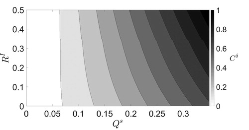
6.1. Determining the optimal C^s

Before using the SKF, we first need to approximate the matrix ${\mathrm{C}}^s$ (see Table 1). To find the optimal value of ${\mathrm{C}}^s$ over the whole assimilation window we carry out numerical experiments for a range of values of ${\mathrm{R}}^I$ and ${\mathrm{Q}}^s.$ Both of these parameters will affect the magnitude of the true large-scale analysis error variance. For each $({\mathrm{R}}^I, {\mathrm{Q}}^s)$ parameter pair, we test a number of values of ${\mathrm{C}}^s$ to determine the value of ${\mathrm{C}}^s$ which gives the smallest true large-scale analysis error variance at the final assimilated observation. As we are calculating the variances only, the calculation is deterministic and the choice of noise realisation is irrelevant. For this experiment, we assimilate 15 observations. We start with ${\mathrm{C}}^s=0$ and increase ${\mathrm{C}}^s$ in steps of $\Delta {\mathrm{C}}^s=0.001$ until ${\mathrm{C}}^s=1.$

The optimal values of ${\mathrm{C}}^s$ that produce the minimum large-scale analysis error variance for the SKF at the final time-step are shown in Fig. 1. The optimal value of ${\mathrm{C}}^s$ increases as both ${\mathrm{R}}^I$ and ${\mathrm{Q}}^s$ increase. In particular, the optimal value of ${\mathrm{C}}^s$ is most sensitive to any increase in ${\mathrm{Q}}^s$ as the error due to unresolved scales is primarily determined by this error variance in our model. While not as sensitive, we find that large ${\mathrm{R}}^I$ also affects the optimal value of ${\mathrm{C}}^s.$ This is because the optimal value of ${\mathrm{C}}^s$ is a function of ${\mathrm{R}}^I$ and ${\mathrm{Q}}^l$ after the initial time. We also find that for small ${\mathrm{R}}^I$ and ${\mathrm{Q}}^s$ the optimal value of ${\mathrm{C}}^s$ over the whole assimilation window is similar to ${\tilde{\mathrm{P}}}^{ss}$ given by equation (5.5)(5.5) $${\tilde{\mathrm{P}}}_k^{ss}=e^{-k}{\tilde{\mathrm{P}}}_0^{ss}+\frac{1-e^{-k}}{1-e^{-1}}{\tilde{\mathrm{Q}}}^s.$$(5.5) for the final time-step. 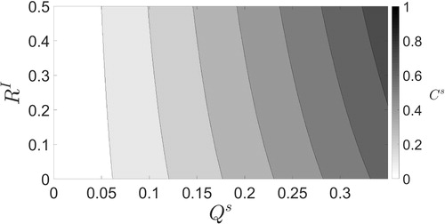For large ${\mathrm{R}}^I$ and ${\mathrm{Q}}^s,$ the optimal value of ${\mathrm{C}}^s$ is approximately 1.4 times larger than ${\tilde{\mathrm{P}}}^{ss}$ evaluated at the final time-step.

Fig. 1. Contour plot of the values of ${\mathrm{C}}^s$ that give the minimum true large-scale analysis error variance at the final assimilated observation for the SKF for different ratios of ${\mathrm{Q}}^s$ and ${\mathrm{R}}^I.$

In operational settings we would not be able to optimise ${\mathrm{C}}^s$ in this way. However, it may be possible to approximate part of the representation error covariance using high resolution observations (Oke and Sakov, 2008) or model data (Waller et al., 2014) and use these approximate representation error values to guide the choice of ${\mathrm{C}}^s.$ To mimic this situation in our experiments, we create an ensemble of 50,000 realizations of x^s for the length of the assimilation windows using the random walk model (5.1)(5.1) $$\begin{array}{c}{\left(\begin{array}{c}{x}^l\\ x^s\end{array}\right)}_{k+1}=\left(\begin{array}{cc}1& 0\\ {\mathrm{M}}^{sl}\mathrm{ }& \hspace{0.17em}\text{exp}\hspace{0.17em}(-1/2)\end{array}\right){\left(\begin{array}{c}{x}^l\\ x^s\end{array}\right)}_k-{\left(\begin{array}{c}{\eta }^l\\ {\eta }^s\end{array}\right)}_k,\\ y_k=\left(\begin{array}{cc}1& 1\end{array}\right){\left(\begin{array}{c}{x}^l\\ x^s\end{array}\right)}_k+{ϵ}_k,\end{array}$$(5.1) and calculate the variance, averaged over the whole ensemble and time. The variance of this ensemble will be denoted $\mathrm{S}$. The variance, $\mathrm{S}$, represents an approximation to the total small-scale variability over the assimilation window. We now compare the values of ${\mathrm{C}}^s$ computed in Fig. 1 with the values of S.

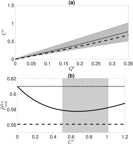
Figure 2(a) shows the optimal ${\mathrm{C}}^s$ values when ${\mathrm{R}}^I=0.1$ (dashed line) and ${\mathrm{R}}^I=0.5$ (dotted line) for different values of ${\mathrm{Q}}^s.$ The grey region shows all points between $\mathrm{S}$ and 2S. As ${\mathrm{Q}}^s$ is increased the variance $\mathrm{S}$ also increases. Both optimal ${\mathrm{C}}^s$ lines lie within the shaded region for nearly all ${\mathrm{Q}}^s.$ We note that when there is little small-scale variability (i.e. ${\mathrm{Q}}^s\approx 0$) the optimal ${\mathrm{C}}^s$ values are less than $\mathrm{S}$ but both are close to zero. Figure 2(b) shows the effect of changing ${\mathrm{C}}^s$ on the SKF true large-scale analysis error variance (solid line) when ${\mathrm{R}}^I=0.1$ and ${\mathrm{Q}}^s=0.35$ in comparison to the true large scale analysis error variances for the RKF and OKF. Thus, for these experiments, a reasonable rule of thumb to avoid areas where the SKF under- or overcompensates for the error due to unresolved scales, is to choose $\mathrm{S}<{\mathrm{C}}^s<2\mathrm{S}.$

Fig. 2. (a): The optimal ${\mathrm{C}}^s$ values when ${\mathrm{R}}^I=0.1$ (dashed line) and ${\mathrm{R}}^I=0.5$ (dotted line) as functions of ${\mathrm{Q}}^s.$ The grey region shows all points between S (lower edge) and 2S (upper edge) for different values of ${\mathrm{Q}}^s.$ (b): The effect of changing ${\mathrm{C}}^s$ on the final true large-scale analysis error covariance for the SKF (solid line) when ${\mathrm{Q}}^s=0.35$ and ${\mathrm{R}}^I=0.1.$ Also shown are the OKF and RKF true large-scale analysis error variance (lower dashed line and upper dotted line respectively). The grey region shows all points between ${\mathrm{C}}^s=\mathrm{S}$ (left edge) and ${\mathrm{C}}^s=2\mathrm{S}$ (right edge). The optimal value of ${\mathrm{C}}^s$ (i.e. the minimum of the solid line) lies in this region.

6.2. Comparison of the SKF with the RKF and OKF

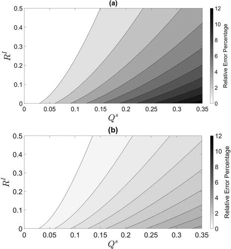
Using the optimal values of ${\mathrm{C}}^s$ calculated in Fig. 1, we now carry out experiments comparing the SKF and RKF for a range of values of ${\mathrm{R}}^I$ and ${\mathrm{Q}}^s$ relative to the OKF. The results are illustrated in terms of relative error percentage for the RKF in Fig. 3a and the SKF in Fig. 3b. The relative error percentage is defined as (6.1) $$\text{relative}\mathrm{ }\text{error}\mathrm{ }\text{percentage}=\frac{\left|{\tilde{\mathrm{P}}}_{\mathit{RKF}/\mathit{SKF}}^{ll,a}-{\tilde{\mathrm{P}}}_{\mathit{OKF}}^{ll,a}\right|}{{\tilde{\mathrm{P}}}_{\mathit{OKF}}^{ll,a}}\times 100\%,$$(6.1) where $|·|$ indicates the absolute value and each term is evaluated at the end of the assimilation window. In these experiments, the SKF always has a true analysis error variance smaller than or equal to the RKF. When there is no error due to unresolved scales (i.e. ${\mathrm{Q}}^s=0$) we have that ${\mathrm{C}}^s=0$ is the optimal value for ${\mathrm{C}}^s$ and the SKF would reduce to the RKF. The largest relative error percentages for both the RKF and SKF occur when there is large uncertainty due to unresolved scales (large ${\mathrm{Q}}^s$) and small ${\mathrm{R}}^I$ and the smallest differences are when ${\mathrm{Q}}^s$ is small. We also find that larger values of ${\mathrm{R}}^I$ limit the difference in performance between the RKF and SKF with the OKF. Therefore, the benefits of using the SKF are most apparent when there is considerable error due to unresolved scales and small instrument error. Comparing Fig. 3a to Fig. 3b we see that, for any fixed value of ${\mathrm{R}}^I,$ as the uncertainty due to unresolved scales is increased the improvement of the SKF over the RKF will also increase.

Fig. 3. (a): Comparison of the RKF to the OKF in terms of relative error percentage given by equation (6.1)(6.1) $$\text{relative}\mathrm{ }\text{error}\mathrm{ }\text{percentage}=\frac{\left|{\tilde{\mathrm{P}}}_{\mathit{RKF}/\mathit{SKF}}^{ll,a}-{\tilde{\mathrm{P}}}_{\mathit{OKF}}^{ll,a}\right|}{{\tilde{\mathrm{P}}}_{\mathit{OKF}}^{ll,a}}\times 100\%,$$(6.1) . (b): Comparison of the SKF with optimal ${\mathrm{C}}^s$ to the OKF at the final time-step in terms of relative error percentage.

To examine the performance perceived by the filter we compare it to the true performance of the filter at the final time-step. Before discussing the results, we note that the SKF perceived analysis error variance will not be a smooth field for the $({\mathrm{R}}^I, {\mathrm{Q}}^s)$ parameter pairs considered. This is because in section 6.1 the optimal value of ${\mathrm{C}}^s$ was calculated to a limited precision of 0.001.

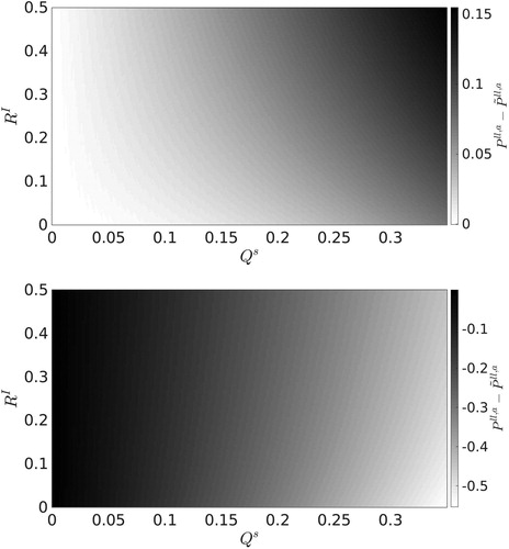
In Fig. 4 we plot the difference between the perceived and true analysis error variance at the final time-step. We note that the magnitude of the difference between the perceived and true error variances is smallest for large ${\mathrm{R}}^I$ and ${\mathrm{Q}}^s.$ Here, the SKF (RKF) perceived error variance is approximately 1.25 (0.5) times the size of the true error variance. The SKF perceived-minus-truth difference shown in panel (a) is always positive for non-negligible representation uncertainty. This shows the SKF is a conservative filtering strategy when compensating for observations exhibiting error due to unresolved scales. As both ${\mathrm{R}}^I$ and ${\mathrm{Q}}^s$ are increased the SKF perceived-minus-truth difference increases. This is due to two reasons. The first reason is because the perceived analysis error variance, ${\mathrm{P}}^{ll,a},$ increases with larger ${\mathrm{C}}^s$ as it is calculated using the short form update (3.2)(3.2) $${\mathbf{P}}_k^a=\left(\mathbf{I}-{\mathbf{K}}_k{\mathbf{H}}_k\right){\mathbf{P}}_k^f,$$(3.2) and the optimal ${\mathrm{C}}^s$ will be larger for higher values of ${\mathrm{R}}^I$ and ${\mathrm{Q}}^s.$ The second reason is because, for non-negligible representation uncertainty, the true analysis error variance, ${\tilde{\mathrm{P}}}^{ll,a},$ will decrease as ${\mathrm{C}}^s$ approaches its optimal value. An illustrative case is provided by Fig. 2b for high representation uncertainty and low instrument uncertainty. Figure 4(b) shows the RKF perceived-minus-truth difference. This is always negative for non-negligible representation uncertainty. This shows the RKF is an overconfident filtering strategy for observations exhibiting error due to unresolved scales. The RKF is most overconfident in regimes of low instrument uncertainty and high representation uncertainty.

Fig. 4. (a): Difference between the perceived and true analysis error variances at the final time-step for the SKF with optimal ${\mathrm{C}}^s.$ (b): Difference between the perceived and true analysis error variances at the final time-step for the RKF.

7. Representation error bias correction through state augmentation

Up to this point we have not considered observation bias in our numerical experiments. However, in operational data assimilation, most observations or their respective observation operators exhibit systematic errors which are referred to as biases. A common approach for correcting observation biases online in a Kalman filter algorithm is to augment the state vector with a bias term (Dee, 2005; Fertig et al., 2009). The bias state will then be estimated and evolved along with the state variables through the data assimilation algorithm (Friedland, 1969).

In section 2.3 we showed that observation errors may exhibit a representation error bias when there is a contribution from the large-scale processes to the small-scale state (i.e., when ${\mathbf{M}}^{sl}\ne {\mathbf{0}}_{N_s\times N_l}$). Throughout the remainder of this manuscript we only consider bias due to unresolved scales which is linked to the state-space representation of the small-scale processes. Since we know the exact form and origin of the observation bias in this study we may treat it as a model bias. Therefore, we consider the augmented state vector x with form (7.1) $$\mathit{x}=\left(\begin{array}{c}{\mathit{x}}^l\\ {\mathit{x}}^{\beta }\end{array}\right),$$(7.1) where ${\mathit{x}}^{\beta }\in {\mathbb{R}}^{N_s}$ is the bias state. Thus, ${\mathit{x}}^{\beta }$ is intended to represent $〈{\mathit{x}}^{s,t}〉$ (cf. (2.13)(2.13) $$〈{\mathbf{H}}^{s,t}{\mathit{x}}_k^{s,t}〉=〈{\mathbf{H}}^{s,t}(\underset{¯}{{\mathbf{M}}^{sl,t}{\mathit{x}}_{k-1}^{l,t}}+{\mathbf{M}}^{s,t}(\underset{¯}{{\mathbf{M}}^{sl,t}{\mathit{x}}_{k-2}^{l,t}}+{\mathbf{M}}^{s,t}(\dots (\underset{¯}{{\mathbf{M}}^{sl,t}{\mathit{x}}_0^{l,t}}+{\mathbf{M}}^{s,t}\left({\mathit{x}}_0^{s,t}\right))\dots )\left)\right)〉,$$(2.13) ). For bias correction through state augmentation we require a prior estimate of the bias and a model to forecast it. Using (2.2)(2.2) $${\left(\begin{array}{c}{\mathit{x}}^{l,t}\\ {\mathit{x}}^{s,t}\end{array}\right)}_k=\left(\begin{array}{cc}{\mathbf{M}}^l& {\mathbf{0}}_{N_l\times N_s}\\ {\mathbf{M}}^{sl}& {\mathbf{M}}^s\end{array}\right){\left(\begin{array}{c}{\mathit{x}}^{l,t}\\ {\mathit{x}}^{s,t}\end{array}\right)}_{k-1}-{\left(\begin{array}{c}{\mathit{\eta }}^l\\ {\mathit{\eta }}^s\end{array}\right)}_k.$$(2.2) , the forecast model for the bias state is given by (7.2) $${\mathit{x}}_k^{\beta }={\mathbf{M}}^{sl}{\mathit{x}}_{k-1}^l+{\mathbf{M}}^s{\mathit{x}}_{k-1}^{\beta },$$(7.2) where we have assumed the model for the bias to be perfect. Random noise can be added to (7.2)(7.2) $${\mathit{x}}_k^{\beta }={\mathbf{M}}^{sl}{\mathit{x}}_{k-1}^l+{\mathbf{M}}^s{\mathit{x}}_{k-1}^{\beta },$$(7.2) to indicate that the bias evolution model is not perfect (Ménard, 2010) but is not explored here. In operational centres the model for individual sources contributing to the bias will be unknown and models describing the total bias will be used instead. These models for the bias will be obtained from assumptions imposed on the bias such as assuming it evolves slowly or is constant in time (e.g., Lea et al., 2008). In cases such as these, the bias estimate will likely be poor as the variation of the bias with the evolution of the large-scale processes will be completely unaccounted for.

We now examine how a bias correction scheme can be implemented in conjunction with the SKF (section 7.1) and the RKF (section 7.2) to correct a bias due to unresolved scales. Table 3 summarizes the components for these two filters which are then substituted into the filter equations detailed in section 3.1.

Table 3. The filter matrices and vectors for the SKFbc and RKFbc. The equations for the the two filters are obtained through substituting these terms into (3.1)(3.1) $${\mathit{x}}_k^a={\mathit{x}}_k^f+{\mathbf{K}}_k{\mathbf{d}}_k^{o,f},$$(3.1) –(3.4)(3.4) $${\mathbf{P}}_{k+1}^f=\mathbf{M}{\mathbf{P}}_k^a{\mathbf{M}}^T+\mathbf{Q},$$(3.4) .

	RKFbc	SKFbc
State: x	$\left(\begin{array}{c}{\mathit{x}}^l\\ {\mathit{x}}^{\beta }\end{array}\right)\in {\mathbb{R}}^{N_t}$	$\left(\begin{array}{c}{\mathit{x}}^l\\ {\mathit{x}}^{\beta }\end{array}\right)\in {\mathbb{R}}^{N_t}$
State error covariance: P	$\left(\begin{array}{cc}{\mathbf{P}}^{ll}& {\mathbf{P}}^{l\beta }\\ {\mathbf{P}}^{\beta l}& {\mathbf{P}}^{\beta \beta }\end{array}\right)\in {\mathbb{R}}^{N_t\times N_t}$	$\left(\begin{array}{ccc}{\mathbf{P}}^{ll}& {\mathbf{P}}^{l\beta }& {\mathbf{P}}^{l\delta }\\ {\mathbf{P}}^{\beta l}& {\mathbf{P}}^{\beta \beta }& {\mathbf{P}}^{\beta \delta }\\ {\mathbf{P}}^{\delta l}& {\mathbf{P}}^{\delta \beta }& {\mathbf{C}}^{\delta }\end{array}\right)\in {\mathbb{R}}^{N_a\times N_a}$
Observation operator: H	$\left(\begin{array}{cc}{\mathbf{H}}^l& {\mathbf{H}}^{\beta }\end{array}\right)\in {\mathbb{R}}^{p\times N_t}$	$\left(\begin{array}{ccc}{\mathbf{H}}^l& {\mathbf{H}}^{\beta }& {\mathbf{H}}^{\delta }\end{array}\right)\in {\mathbb{R}}^{p\times N_a}$
Observation error covariance: R	${\mathbf{R}}^I+{\mathbf{R}}^H\in {\mathbb{R}}^{p\times p}$	${\mathbf{R}}^I+{\mathbf{R}}^G\in {\mathbb{R}}^{p\times p}$
Innovation: ${\mathbf{d}}^{o,f}$	$\mathit{y}-\left(\begin{array}{cc}{\mathbf{H}}^l& {\mathbf{H}}^{\beta }\end{array}\right)\left(\begin{array}{c}{\mathit{x}}^{l,f}\\ {\mathit{x}}^{\beta ,f}\end{array}\right)$	$\mathit{y}-\left(\begin{array}{cc}{\mathbf{H}}^l& {\mathbf{H}}^{\beta }\end{array}\right)\left(\begin{array}{c}{\mathit{x}}^{l,f}\\ {\mathit{x}}^{\beta ,f}\end{array}\right)$
Innovation covariance: D	$\left(\begin{array}{cc}{\mathbf{H}}^l& {\mathbf{H}}^{\beta }\end{array}\right)\left(\begin{array}{cc}{\mathbf{P}}^{ll,f}& {\mathbf{P}}^{l\beta ,f}\\ {\mathbf{P}}^{\beta l,f}& {\mathbf{P}}^{\beta \beta ,f}\end{array}\right)\left(\begin{array}{c}{\left({\mathbf{H}}^l\right)}^T\\ {\left({\mathbf{H}}^{\beta }\right)}^T\end{array}\right)+\mathbf{R}$	$\left(\begin{array}{ccc}{\mathbf{H}}^l& {\mathbf{H}}^{\beta }& {\mathbf{H}}^{\delta }\end{array}\right)\left(\begin{array}{ccc}{\mathbf{P}}^{ll,f}& {\mathbf{P}}^{l\beta ,f}& {\mathbf{P}}^{l\delta ,f}\\ {\mathbf{P}}^{\beta l,f}& {\mathbf{P}}^{\beta \beta ,f}& {\mathbf{P}}^{\beta \delta ,f}\\ {\mathbf{P}}^{\delta l,f}& {\mathbf{P}}^{\delta \beta ,f}& {\mathbf{C}}^{\delta }\end{array}\right)\left(\begin{array}{c}{\left({\mathbf{H}}^l\right)}^T\\ {\left({\mathbf{H}}^{\beta }\right)}^T\\ {\left({\mathbf{H}}^{\delta }\right)}^T\end{array}\right)+\mathbf{R}$
Kalman gain: K	$\left(\begin{array}{c}{\mathbf{K}}^l\\ {\mathbf{K}}^{\beta }\end{array}\right)=\left(\begin{array}{cc}{\mathbf{P}}^{ll,f}& {\mathbf{P}}^{l\beta ,f}\\ {\mathbf{P}}^{\beta l,f}& {\mathbf{P}}^{\beta \beta ,f}\end{array}\right)\left(\begin{array}{c}{\left({\mathbf{H}}^l\right)}^T\\ {\left({\mathbf{H}}^{\beta }\right)}^T\end{array}\right){\mathbf{D}}^{-1}$	$\begin{array}{c}\text{State}\mathrm{ }\text{update}\hfill \\ \left(\begin{array}{c}{\mathbf{K}}^l\\ {\mathbf{K}}^{\beta }\end{array}\right)=\left(\begin{array}{c}{\mathbf{P}}^{ll,f}{\left({\mathbf{H}}^l\right)}^T+{\mathbf{P}}^{l\beta ,f}{\left({\mathbf{H}}^{\beta }\right)}^T+{\mathbf{P}}^{l\delta ,f}{\left({\mathbf{H}}^{\delta }\right)}^T\\ {\mathbf{P}}^{\beta l,f}{\left({\mathbf{H}}^l\right)}^T+{\mathbf{P}}^{\beta \beta ,f}{\left({\mathbf{H}}^{\beta }\right)}^T+{\mathbf{P}}^{\beta \delta ,f}{\left({\mathbf{H}}^{\delta }\right)}^T\end{array}\right){\mathbf{D}}^{-1}\hfill \\ \text{Covariance}\mathrm{ }\text{update}\hfill \\ \left(\begin{array}{c}{\mathbf{K}}^l\\ {\mathbf{K}}^{\beta }\\ {\mathbf{K}}^{\delta }\end{array}\right)=\left(\begin{array}{c}{\mathbf{P}}^{ll,f}{\left({\mathbf{H}}^l\right)}^T+{\mathbf{P}}^{l\beta ,f}{\left({\mathbf{H}}^{\beta }\right)}^T+{\mathbf{P}}^{l\delta ,f}{\left({\mathbf{H}}^{\delta }\right)}^T\\ {\mathbf{P}}^{\beta l,f}{\left({\mathbf{H}}^l\right)}^T+{\mathbf{P}}^{\beta \beta ,f}{\left({\mathbf{H}}^{\beta }\right)}^T+{\mathbf{P}}^{\beta \delta ,f}{\left({\mathbf{H}}^{\delta }\right)}^T\\ {\mathbf{0}}_{N_s\times p}\end{array}\right){\mathbf{D}}^{-1}\hfill \end{array}$
Forecast model: M	$\left(\begin{array}{cc}{\mathbf{M}}^l& {\mathbf{0}}_{N_l\times N_s}\\ {\mathbf{M}}^{sl}& {\mathbf{M}}^s\end{array}\right)\in {\mathbb{R}}^{N_t\times N_t}$	$\begin{array}{c}\text{State}\mathrm{ }\text{update}\\ \left(\begin{array}{cc}{\mathbf{M}}^l& {\mathbf{0}}_{N_l\times N_s}\\ {\mathbf{M}}^{sl}& {\mathbf{M}}^s\end{array}\right)\in {\mathrm{ℝ}}^{N_l\times N_l}\\ \text{Covariance}\mathrm{ }\text{update}\\ \left(\begin{array}{ccc}{\mathbf{M}}^l& {\mathbf{0}}_{N_l\times N_s}& {\mathbf{0}}_{N_l\times N_s}\\ {\mathbf{M}}^{sl}& {\mathbf{M}}^s& {\mathbf{0}}_{N_s\times N_s}\\ {\mathbf{0}}_{N_s\times N_l}& {\mathbf{0}}_{N_s\times N_s}& {\mathbf{M}}^s\end{array}\right)\in {\mathrm{ℝ}}^{N_a\times N_a}\end{array}$
Model error covariance: Q	$\left(\begin{array}{cc}{\mathbf{Q}}^{ll}& {\mathbf{0}}_{N_l\times N_s}\\ {\mathbf{0}}_{N_s\times N_l}& {\mathbf{0}}_{N_s\times N_s}\end{array}\right)\in {\mathbb{R}}^{N_t\times N_t}$	$\left(\begin{array}{ccc}{\mathbf{Q}}^{ll}& {\mathbf{0}}_{N_l\times N_s}& {\mathbf{Q}}^{ls}\\ {\mathbf{0}}_{N_s\times N_l}& {\mathbf{0}}_{N_s\times N_s}& {\mathbf{0}}_{N_s\times N_s}\\ {\mathbf{Q}}^{sl}& {\mathbf{0}}_{N_s\times N_s}& {\mathbf{Q}}^{ss}\end{array}\right)\in {\mathrm{ℝ}}^{N_a\times N_a}$

7.1. The Schmidt-Kalman filter with observational bias correction

Bias correction through state augmentation is a common method used in operational centres but use of a bias correction scheme with the SKF, which will be denoted SKFbc, is novel.

We assume that we have knowledge of the processes for all scales. We further assume that we have a model and prior estimate for the bias. The filtered state vector for the SKFbc is given by equation (7.1)(7.1) $$\mathit{x}=\left(\begin{array}{c}{\mathit{x}}^l\\ {\mathit{x}}^{\beta }\end{array}\right),$$(7.1) and only includes the large-scale state and the bias term. The small-scale state is split into a biased and unbiased component, i.e. (7.3) $${\mathit{x}}^s={\mathit{x}}^{\beta }+{\mathit{x}}^{\delta },$$(7.3) such that $〈{\mathit{x}}^s〉={\mathit{x}}^{\beta }.$ The unbiased small-scale processes, ${\mathit{x}}^{\delta },$ will be accounted for through their statistics. The full observation operator for the SKFbc is given by (7.4) $$\left(\begin{array}{ccc}{\mathbf{H}}^l& {\mathbf{H}}^{\beta }& {\mathbf{H}}^{\delta }\end{array}\right)\in {\mathbb{R}}^{p\times N_a},$$(7.4) where ${\mathbf{H}}^{\beta }\in {\mathbb{R}}^{p\times N_s}$ and ${\mathbf{H}}^{\delta }\in {\mathbb{R}}^{p\times N_s}$ are the linear observation operators which map the bias and unbiased small-scale states into observation space respectively. However, as with the SKF, the analysis update equation (3.1)(3.1) $${\mathit{x}}_k^a={\mathit{x}}_k^f+{\mathbf{K}}_k{\mathbf{d}}_k^{o,f},$$(3.1) uses a forecast innovation that takes no account of the unbiased small-scales, (7.5) $${\mathbf{d}}^{o,f}=\mathit{y}-\left(\begin{array}{cc}{\mathbf{H}}^l& {\mathbf{H}}^{\beta }\end{array}\right)\left(\begin{array}{c}{\mathit{x}}^{l,f}\\ {\mathit{x}}^{\beta ,f}\end{array}\right).$$(7.5)

This innovation is unbiased and hence the large-scale analysis errors are also unbiased. The Kalman gain for the SKFbc consists of a large-scale gain ${\mathbf{K}}^l\in {\mathbb{R}}^{N_l\times p}$ and a bias estimate gain ${\mathbf{K}}^{\beta }\in {\mathbb{R}}^{N_s\times p}$ given by (7.6) $$\left(\begin{array}{c}{\mathbf{K}}^l\\ {\mathbf{K}}^{\beta }\end{array}\right)=\left(\begin{array}{c}{\mathbf{P}}^{ll,f}{({\mathbf{H}}^l)}^T+{\mathbf{P}}^{l\beta ,f}{({\mathbf{H}}^{\beta })}^T+{\mathbf{P}}^{l\delta ,f}{({\mathbf{H}}^{\delta })}^T\\ {\mathbf{P}}^{\beta l,f}{({\mathbf{H}}^l)}^T+{\mathbf{P}}^{\beta \beta ,f}{({\mathbf{H}}^{\beta })}^T+{\mathbf{P}}^{\beta \delta ,f}{({\mathbf{H}}^{\delta })}^T\end{array}\right){\mathbf{D}}^{-1},$$(7.6) where ${\mathbf{P}}^{l\beta }\in {\mathbb{R}}^{N_l\times N_s}$ is the perceived cross-covariance between the large-scale errors and bias estimate errors, ${\mathbf{P}}^{l\delta }\in {\mathbb{R}}^{N_l\times N_s}$ is the perceived cross-covariance between the large-scale errors and unbiased small-scale errors, ${\mathbf{P}}^{\beta \beta }\in {\mathbb{R}}^{N_s\times N_s}$ is the perceived covariance of the bias estimate errors and ${\mathbf{P}}^{\beta \delta }\in {\mathbb{R}}^{N_s\times N_s}$ is the perceived cross-covariance between the bias estimate errors and unbiased small-scale errors. The perceived augmented innovation covariance D is given in Table 3. This increases the uncertainty the filter attributes to the forecast innovation compared with the standard SKF. The additional uncertainty is a result of the errors accrued in the estimation of the bias. The term ${\mathbf{H}}^s{\mathbf{C}}^{\delta }{({\mathbf{H}}^s)}^T$ in the SKFbc innovation error covariance corresponds to the variability of the unbiased small-scale processes.

The SKFbc equations are obtained from augmenting the large-scale terms with bias terms and defining the cross-covariance terms appropriately. The analysis state update for the SKFbc is then (7.7) $${\left(\begin{array}{c}{\mathit{x}}^{l,a}\\ {\mathit{x}}^{\beta ,a}\end{array}\right)}_k={\left(\begin{array}{c}{\mathit{x}}^{l,f}\\ {\mathit{x}}^{\beta ,f}\end{array}\right)}_k+{\left(\begin{array}{c}{\mathbf{K}}^l\\ {\mathbf{K}}^{\beta }\end{array}\right)}_k\left({\mathit{y}}_k-{\left(\begin{array}{cc}{\mathbf{H}}^l& {\mathbf{H}}^{\beta }\end{array}\right)}_k{\left(\begin{array}{c}{\mathit{x}}^{l,f}\\ {\mathit{x}}^{\beta ,f}\end{array}\right)}_k\right).$$(7.7)

To obtain the analysis error covariance update we augment the gain (7.6)(7.6) $$\left(\begin{array}{c}{\mathbf{K}}^l\\ {\mathbf{K}}^{\beta }\end{array}\right)=\left(\begin{array}{c}{\mathbf{P}}^{ll,f}{({\mathbf{H}}^l)}^T+{\mathbf{P}}^{l\beta ,f}{({\mathbf{H}}^{\beta })}^T+{\mathbf{P}}^{l\delta ,f}{({\mathbf{H}}^{\delta })}^T\\ {\mathbf{P}}^{\beta l,f}{({\mathbf{H}}^l)}^T+{\mathbf{P}}^{\beta \beta ,f}{({\mathbf{H}}^{\beta })}^T+{\mathbf{P}}^{\beta \delta ,f}{({\mathbf{H}}^{\delta })}^T\end{array}\right){\mathbf{D}}^{-1},$$(7.6) with ${\mathbf{K}}^{\delta }={\mathbf{0}}_{N_s\times p}$ and substitute into the short-form analysis error covariance update (3.2)(3.2) $${\mathbf{P}}_k^a=\left(\mathbf{I}-{\mathbf{K}}_k{\mathbf{H}}_k\right){\mathbf{P}}_k^f,$$(3.2) . To mirror the SKF analysis error covariance update equations (3.12)-(3.14), we express the SKFbc analysis error covariance update equations as (7.8) $${\left(\begin{array}{cc}{\mathbf{P}}^{ll,a}& {\mathbf{P}}^{l\beta ,a}\\ {\mathbf{P}}^{\beta l,a}& {\mathbf{P}}^{\beta \beta ,a}\end{array}\right)}_k={\left(\begin{array}{cc}{\mathbf{I}}_{N_l}-{\mathbf{K}}^l{\mathbf{H}}^l& -{\mathbf{K}}^l{\mathbf{H}}^{\beta }\\ -{\mathbf{K}}^{\beta }{\mathbf{H}}^l& {\mathbf{I}}_{N_s}-{\mathbf{K}}^{\beta }{\mathbf{H}}^{\beta }\end{array}\right)}_k{\left(\begin{array}{cc}{\mathbf{P}}^{ll,f}& {\mathbf{P}}^{l\beta ,f}\\ {\mathbf{P}}^{\beta l,f}& {\mathbf{P}}^{\beta \beta ,f}\end{array}\right)}_k-{\left(\begin{array}{cc}{\mathbf{K}}^l{\mathbf{H}}^{\delta }{\mathbf{P}}^{\delta l,f}& {\mathbf{K}}^l{\mathbf{H}}^{\delta }{\mathbf{P}}^{\delta \beta ,f}\\ {\mathbf{K}}^{\beta }{\mathbf{H}}^{\delta }{\mathbf{P}}^{\delta l,f}& {\mathbf{K}}^{\beta }{\mathbf{H}}^{\delta }{\mathbf{P}}^{\delta \beta ,f}\end{array}\right)}_k,$$(7.8) (7.9) $${\left(\begin{array}{c}{\mathbf{P}}^{l\delta ,a}\\ {\mathbf{P}}^{\beta \delta ,a}\end{array}\right)}_k={\left(\begin{array}{cc}{\mathbf{I}}_{N_l}-{\mathbf{K}}^l{\mathbf{H}}^l& -{\mathbf{K}}^l{\mathbf{H}}^{\beta }\\ -{\mathbf{K}}^{\beta }{\mathbf{H}}^l& {\mathbf{I}}_{N_s}-{\mathbf{K}}^{\beta }{\mathbf{H}}^{\beta }\end{array}\right)}_k{\left(\begin{array}{c}{\mathbf{P}}^{l\delta ,f}\\ {\mathbf{P}}^{\beta \delta ,f}\end{array}\right)}_k-{\left(\begin{array}{c}{\mathbf{K}}^l{\mathbf{H}}^{\delta }{\mathbf{C}}^{\delta }\\ {\mathbf{K}}^{\beta }{\mathbf{H}}^{\delta }{\mathbf{C}}^{\delta }\end{array}\right)}_k,$$(7.9) (7.10) $${\left(\begin{array}{cc}{\mathbf{P}}^{\delta l,a}& {\mathbf{P}}^{\delta \beta ,a}\end{array}\right)}_k={\left(\begin{array}{cc}{\left({\mathbf{P}}^{l\delta ,a}\right)}^T& {\left({\mathbf{P}}^{\beta \delta ,a}\right)}^T\end{array}\right)}_k.$$(7.10)

Since in the context of the SKFbc the complete model evolving all scales is assumed to be known, it is appropriate to update the bias term using this model (7.2)(7.2) $${\mathit{x}}_k^{\beta }={\mathbf{M}}^{sl}{\mathit{x}}_{k-1}^l+{\mathbf{M}}^s{\mathit{x}}_{k-1}^{\beta },$$(7.2) . Thus, the forecast state update is given by (7.11) $${\left(\begin{array}{c}{\mathit{x}}^{l,f}\\ {\mathit{x}}^{\beta ,f}\end{array}\right)}_{k+1}=\left(\begin{array}{cc}{\mathbf{M}}^l& {\mathbf{0}}_{N_l\times N_s}\\ {\mathbf{M}}^{sl}& {\mathbf{M}}^s\end{array}\right){\left(\begin{array}{c}{\mathit{x}}^{l,a}\\ {\mathit{x}}^{\beta ,a}\end{array}\right)}_k.$$(7.11)

For the forecast error covariance we need the model for the unbiased small-scale processes. To determine this model we use the definition (7.3)(7.3) $${\mathit{x}}^s={\mathit{x}}^{\beta }+{\mathit{x}}^{\delta },$$(7.3) together with the bias evolution equation (7.2)(7.2) $${\mathit{x}}_k^{\beta }={\mathbf{M}}^{sl}{\mathit{x}}_{k-1}^l+{\mathbf{M}}^s{\mathit{x}}_{k-1}^{\beta },$$(7.2) , to give (7.12) $${\mathit{x}}_k^{\delta }={\mathbf{M}}^s{\mathit{x}}_{k-1}^{\delta }+{\mathit{\eta }}_k^s.$$(7.12)

Note that the small-scale model error ${\mathit{\eta }}_{}^s$ is assumed to be unbiased. To mirror the SKF forecast error covariance update equations (3.16)-(3.18), we express the SKFbc forecast error covariance updates as (7.13) $${\left(\begin{array}{cc}{\mathbf{P}}^{ll,f}& {\mathbf{P}}^{l\beta ,f}\\ {\mathbf{P}}^{\beta l,f}& {\mathbf{P}}^{\beta \beta ,f}\end{array}\right)}_{k+1}=\left(\begin{array}{cc}{\mathbf{M}}^l& {\mathbf{0}}_{N_l\times N_s}\\ {\mathbf{M}}^{sl}& {\mathbf{M}}^s\end{array}\right){\left(\begin{array}{cc}{\mathbf{P}}^{ll,a}& {\mathbf{P}}^{l\beta ,a}\\ {\mathbf{P}}^{\beta l,a}& {\mathbf{P}}^{\beta \beta ,a}\end{array}\right)}_k{\left(\begin{array}{cc}{\mathbf{M}}^l& {\mathbf{0}}_{N_l\times N_s}\\ {\mathbf{M}}^{sl}& {\mathbf{M}}^s\end{array}\right)}^T+\left(\begin{array}{cc}{\mathbf{Q}}^{ll}& {\mathbf{0}}_{N_l\times N_s}\\ {\mathbf{0}}_{N_s\times N_l}& {\mathbf{0}}_{N_s\times N_s}\end{array}\right),$$(7.13) (7.14) $${\left(\begin{array}{c}{\mathbf{P}}^{l\delta ,f}\\ {\mathbf{P}}^{\beta \delta ,f}\end{array}\right)}_{k+1}=\left(\begin{array}{cc}{\mathbf{M}}^l& {\mathbf{0}}_{N_l\times N_s}\\ {\mathbf{M}}^{sl}& {\mathbf{M}}^s\end{array}\right){\left(\begin{array}{c}{\mathbf{P}}^{l\delta ,a}\\ {\mathbf{P}}^{\beta \delta ,a}\end{array}\right)}_k{\left({\mathbf{M}}^s\right)}^T,$$(7.14) (7.15) $${\left(\begin{array}{cc}{\mathbf{P}}^{\delta l,f}& {\mathbf{P}}^{\delta \beta ,f}\end{array}\right)}_{k+1}={\left(\begin{array}{c}{\mathbf{P}}^{l\delta ,f}\\ {\mathbf{P}}^{\beta \delta ,f}\end{array}\right)}_{k+1}^T.$$(7.15)

The prescribed unbiased small-scale error covariance ${\mathbf{C}}^{\delta }$ is assumed constant in time and is not updated.

The SKFbc allows us to correct biases due to unresolved scales and consider the effects of the unbiased small-scale processes on the large-scale state. A key advantage in this method is that the cross-correlations between the large-scale errors and small-scale errors are retained. However, the SKF is a computationally expensive procedure. This issue is exacerbated by the use of state augmentation for bias correction.

7.2. The reduced-state Kalman filter with observation bias correction

To save on the computational expense incurred by the SKFbc we can disregard the unbiased small-scale processes to obtain the reduced-state Kalman filter with bias correction (RKFbc). As before, we augment the large scale state vector with a bias term, so that the estimated state is given by (7.1)(7.1) $$\mathit{x}=\left(\begin{array}{c}{\mathit{x}}^l\\ {\mathit{x}}^{\beta }\end{array}\right),$$(7.1) . The observation operator is also augmented and takes the form, (7.16) $$\mathbf{H}=\left(\begin{array}{cc}{\mathbf{H}}^l& {\mathbf{H}}^{\beta }\end{array}\right).$$(7.16)

As with the SKFbc, the forecast innovation (7.5)(7.5) $${\mathbf{d}}^{o,f}=\mathit{y}-\left(\begin{array}{cc}{\mathbf{H}}^l& {\mathbf{H}}^{\beta }\end{array}\right)\left(\begin{array}{c}{\mathit{x}}^{l,f}\\ {\mathit{x}}^{\beta ,f}\end{array}\right).$$(7.5) used in the analysis update (3.1)(3.1) $${\mathit{x}}_k^a={\mathit{x}}_k^f+{\mathbf{K}}_k{\mathbf{d}}_k^{o,f},$$(3.1) takes no account of unbiased small scale error. Therefore, a properly specified observation error covariance for the RKFbc contains both instrument error and representation error (i.e. $\mathbf{R}={\mathbf{R}}^I+{\mathbf{R}}^H$).

Similarly to the SKFbc, the Kalman gain for the RKFbc consists of a large-scale gain ${\mathbf{K}}^l\in {\mathbb{R}}^{N_l\times p}$ and a bias estimate gain ${\mathbf{K}}^{\beta }\in {\mathbb{R}}^{N_s\times p}$ given by (7.17) $$\left(\begin{array}{c}{\mathbf{K}}^l\\ {\mathbf{K}}^{\beta }\end{array}\right)=\left(\begin{array}{c}{\mathbf{P}}^{ll,f}{({\mathbf{H}}^l)}^T+{\mathbf{P}}^{l\beta ,f}{({\mathbf{H}}^{\beta })}^T\\ {\mathbf{P}}^{\beta l,f}{({\mathbf{H}}^l)}^T+{\mathbf{P}}^{\beta \beta ,f}{({\mathbf{H}}^{\beta })}^T\end{array}\right){\mathbf{D}}^{-1},$$(7.17) where the perceived innovation covariance $\mathbf{D}\in {\mathbb{R}}^{p\times p}$ is given in Table 3. Thus, the analysis state update for the RKFbc is obtained through substitution of the gain matrix (7.17)(7.17) $$\left(\begin{array}{c}{\mathbf{K}}^l\\ {\mathbf{K}}^{\beta }\end{array}\right)=\left(\begin{array}{c}{\mathbf{P}}^{ll,f}{({\mathbf{H}}^l)}^T+{\mathbf{P}}^{l\beta ,f}{({\mathbf{H}}^{\beta })}^T\\ {\mathbf{P}}^{\beta l,f}{({\mathbf{H}}^l)}^T+{\mathbf{P}}^{\beta \beta ,f}{({\mathbf{H}}^{\beta })}^T\end{array}\right){\mathbf{D}}^{-1},$$(7.17) and forecast innovation (7.5)(7.5) $${\mathbf{d}}^{o,f}=\mathit{y}-\left(\begin{array}{cc}{\mathbf{H}}^l& {\mathbf{H}}^{\beta }\end{array}\right)\left(\begin{array}{c}{\mathit{x}}^{l,f}\\ {\mathit{x}}^{\beta ,f}\end{array}\right).$$(7.5) into the linear filter analysis state update equation (3.1)(3.1) $${\mathit{x}}_k^a={\mathit{x}}_k^f+{\mathbf{K}}_k{\mathbf{d}}_k^{o,f},$$(3.1) . Likewise, the analysis error covariance update equation is obtained through substitution of the gain matrix (7.17)(7.17) $$\left(\begin{array}{c}{\mathbf{K}}^l\\ {\mathbf{K}}^{\beta }\end{array}\right)=\left(\begin{array}{c}{\mathbf{P}}^{ll,f}{({\mathbf{H}}^l)}^T+{\mathbf{P}}^{l\beta ,f}{({\mathbf{H}}^{\beta })}^T\\ {\mathbf{P}}^{\beta l,f}{({\mathbf{H}}^l)}^T+{\mathbf{P}}^{\beta \beta ,f}{({\mathbf{H}}^{\beta })}^T\end{array}\right){\mathbf{D}}^{-1},$$(7.17) into the short form analysis error covariance update (3.2)(3.2) $${\mathbf{P}}_k^a=\left(\mathbf{I}-{\mathbf{K}}_k{\mathbf{H}}_k\right){\mathbf{P}}_k^f,$$(3.2) along with the observation operator (7.16)(7.16) $$\mathbf{H}=\left(\begin{array}{cc}{\mathbf{H}}^l& {\mathbf{H}}^{\beta }\end{array}\right).$$(7.16) .

For the RKF we assumed knowledge of the large-scale processes only. Hence, the model for the bias due to unresolved scales would be unknown and further assumptions required for the observation bias correction scheme. Nevertheless, to provide a direct comparison we will use the same model as the SKFbc (7.11)(7.11) $${\left(\begin{array}{c}{\mathit{x}}^{l,f}\\ {\mathit{x}}^{\beta ,f}\end{array}\right)}_{k+1}=\left(\begin{array}{cc}{\mathbf{M}}^l& {\mathbf{0}}_{N_l\times N_s}\\ {\mathbf{M}}^{sl}& {\mathbf{M}}^s\end{array}\right){\left(\begin{array}{c}{\mathit{x}}^{l,a}\\ {\mathit{x}}^{\beta ,a}\end{array}\right)}_k.$$(7.11) for the forecast state update. This model and a consistent model error covariance matrix (see Table 3) are used for the augmented analysis error covariance update (3.2)(3.2) $${\mathbf{P}}_k^a=\left(\mathbf{I}-{\mathbf{K}}_k{\mathbf{H}}_k\right){\mathbf{P}}_k^f,$$(3.2) .

Comparison of the OKF column in table 1 and the RKFbc column in table 3 shows the two filters have similar components as a result of the bias correction through state augmentation approach. The key difference between the two filters is the model error covariance expressions. The OKF accounts for the uncertainty in all scales and so uses the full model error covariance. The RKFbc accounts for the uncertainty in the large-scales and the estimate of the bias. Since the model for the bias (7.2)(7.2) $${\mathit{x}}_k^{\beta }={\mathbf{M}}^{sl}{\mathit{x}}_{k-1}^l+{\mathbf{M}}^s{\mathit{x}}_{k-1}^{\beta },$$(7.2) has been assumed perfect the RKFbc will only account for large-scale model error. We note that, as no knowledge of the small-scale processes is assumed for the RKFbc, the forecast model will differ in practice from that of the OKF as the RKFbc bias forecast model would come from additional assumptions placed on the bias.

The RKFbc is a computationally cheaper alternative to the SKFbc for online bias correction that takes no account of unbiased small-scale errors, except through the choice of observation error covariance.

7.3. True analysis error equations for bias correcting filters

The true analysis error equation for the SKFbc and RKFbc will differ from the case 2 true analysis error equation (4.4)(4.4) $${\mathbf{e}}_k^{l,a}\equiv {\mathit{x}}_k^{l,a}-{\mathit{x}}_k^{l,t}\mathrm{ }=\left(\begin{array}{c}{\mathbf{I}}_{N_l}-{\mathbf{K}}_k^l{\mathbf{H}}_k^l\end{array}\right){\mathbf{M}}^l{\mathbf{e}}_{k-1}^{l,a}+\left(\begin{array}{c}{\mathbf{I}}_{N_l}-{\mathbf{K}}_k^l{\mathbf{H}}_k^l\end{array}\right){\mathit{\eta }}_k^l+{\mathbf{K}}_k^l({\mathit{ϵ}}_k+{\mathit{\gamma }}_k^l+{\mathbf{H}}_k^{s,t}{\mathit{x}}_k^{s,t}).$$(4.4) due to the innovation (7.5)(7.5) $${\mathbf{d}}^{o,f}=\mathit{y}-\left(\begin{array}{cc}{\mathbf{H}}^l& {\mathbf{H}}^{\beta }\end{array}\right)\left(\begin{array}{c}{\mathit{x}}^{l,f}\\ {\mathit{x}}^{\beta ,f}\end{array}\right).$$(7.5) . The change will only be in the large-scale part of the true analysis error equations as the small-scale state is not analysed by either filter. The large-scale true analysis error equation for the bias correction filters is obtained from subtracting ${\mathbf{K}}_k^l{\mathbf{H}}^{\beta }{\mathit{x}}_k^{\beta ,f}$ from the case 2 true analysis error equation (4.4)(4.4) $${\mathbf{e}}_k^{l,a}\equiv {\mathit{x}}_k^{l,a}-{\mathit{x}}_k^{l,t}\mathrm{ }=\left(\begin{array}{c}{\mathbf{I}}_{N_l}-{\mathbf{K}}_k^l{\mathbf{H}}_k^l\end{array}\right){\mathbf{M}}^l{\mathbf{e}}_{k-1}^{l,a}+\left(\begin{array}{c}{\mathbf{I}}_{N_l}-{\mathbf{K}}_k^l{\mathbf{H}}_k^l\end{array}\right){\mathit{\eta }}_k^l+{\mathbf{K}}_k^l({\mathit{ϵ}}_k+{\mathit{\gamma }}_k^l+{\mathbf{H}}_k^{s,t}{\mathit{x}}_k^{s,t}).$$(4.4) which produces (7.18) $${\mathbf{e}}_k^{l,a}=\left(\begin{array}{c}{\mathbf{I}}_{N_l}-{\mathbf{K}}_k^l{\mathbf{H}}_k^l\end{array}\right){\mathbf{M}}^l{\mathbf{e}}_{k-1}^{l,a}+\left(\begin{array}{c}{\mathbf{I}}_{N_l}-{\mathbf{K}}_k^l{\mathbf{H}}_k^l\end{array}\right){\mathit{\eta }}_k^l+{\mathbf{K}}_k^l({\mathit{ϵ}}_k+{\mathit{\gamma }}_k^l+{\mathbf{H}}_k^{s,t}{\mathit{x}}_k^{s,t}-{\mathbf{H}}_k^{\beta }{\mathit{x}}_k^{\beta ,f}).$$(7.18)

The true large-scale analysis error covariance for the bias correcting filters is then given by (7.19) $$\begin{array}{c}{\tilde{\mathbf{P}}}_k^{ll,a}=\left({\mathbf{I}}_{N_l}-{\mathbf{K}}_k^l{\mathbf{H}}_k^l\right){\tilde{\mathbf{P}}}_k^{ll,f}{\left({\mathbf{I}}_{N_l}-{\mathbf{K}}_k^l{\mathbf{H}}_k^l\right)}^T\\ \mathrm{\hspace{1em}}\mathrm{\hspace{1em}}+{\mathbf{K}}_k^l\left({\tilde{\mathbf{R}}}_k^I+\left({\mathbf{H}}_k^{s,t}{\mathit{x}}_k^{s,t}-{\mathbf{H}}_k^{\beta }{\mathit{x}}_k^{\beta ,f}\right){\left({\mathbf{H}}_k^{s,t}{\mathit{x}}_k^{s,t}-{\mathbf{H}}_k^{\beta }{\mathit{x}}_k^{\beta ,f}\right)}^T\right){\left({\mathbf{K}}_k^l\right)}^T.\end{array}$$(7.19)

The difference between the true analysis error covariance for the non-bias correcting filters and (7.19)(7.19) $$\begin{array}{c}{\tilde{\mathbf{P}}}_k^{ll,a}=\left({\mathbf{I}}_{N_l}-{\mathbf{K}}_k^l{\mathbf{H}}_k^l\right){\tilde{\mathbf{P}}}_k^{ll,f}{\left({\mathbf{I}}_{N_l}-{\mathbf{K}}_k^l{\mathbf{H}}_k^l\right)}^T\\ \mathrm{\hspace{1em}}\mathrm{\hspace{1em}}+{\mathbf{K}}_k^l\left({\tilde{\mathbf{R}}}_k^I+\left({\mathbf{H}}_k^{s,t}{\mathit{x}}_k^{s,t}-{\mathbf{H}}_k^{\beta }{\mathit{x}}_k^{\beta ,f}\right){\left({\mathbf{H}}_k^{s,t}{\mathit{x}}_k^{s,t}-{\mathbf{H}}_k^{\beta }{\mathit{x}}_k^{\beta ,f}\right)}^T\right){\left({\mathbf{K}}_k^l\right)}^T.\end{array}$$(7.19) is that ${\tilde{\mathbf{R}}}_k^H$ has been replaced with $({\mathbf{H}}_k^{s,t}{\mathit{x}}_k^{s,t}-{\mathbf{H}}_k^{\beta }{\mathit{x}}_k^{\beta ,f}){({\mathbf{H}}_k^{s,t}{\mathit{x}}_k^{s,t}-{\mathbf{H}}_k^{\beta }{\mathit{x}}_k^{\beta ,f})}^T$ which corresponds to the uncertainty due to unresolved scales and the uncertainty in the estimate of the bias. Similarly to (4.5)(4.5) $${\tilde{\mathbf{P}}}_k^{ll,a}\equiv 〈{\mathbf{e}}_k^{l,a}{({\mathbf{e}}_k^{l,a})}^T〉=\left({\mathbf{I}}_{N_l}-{\mathbf{K}}_k^l{\mathbf{H}}_k^l\right){\tilde{\mathbf{P}}}_k^{ll,f}{\left({\mathbf{I}}_{N_l}-{\mathbf{K}}_k^l{\mathbf{H}}_k^l\right)}^T+{\mathbf{K}}_k^l\left({\tilde{\mathbf{R}}}_k^I+{\tilde{\mathbf{R}}}_k^H\right){\left({\mathbf{K}}_k^l\right)}^T.$$(4.5) , equation (7.19)(7.19) $$\begin{array}{c}{\tilde{\mathbf{P}}}_k^{ll,a}=\left({\mathbf{I}}_{N_l}-{\mathbf{K}}_k^l{\mathbf{H}}_k^l\right){\tilde{\mathbf{P}}}_k^{ll,f}{\left({\mathbf{I}}_{N_l}-{\mathbf{K}}_k^l{\mathbf{H}}_k^l\right)}^T\\ \mathrm{\hspace{1em}}\mathrm{\hspace{1em}}+{\mathbf{K}}_k^l\left({\tilde{\mathbf{R}}}_k^I+\left({\mathbf{H}}_k^{s,t}{\mathit{x}}_k^{s,t}-{\mathbf{H}}_k^{\beta }{\mathit{x}}_k^{\beta ,f}\right){\left({\mathbf{H}}_k^{s,t}{\mathit{x}}_k^{s,t}-{\mathbf{H}}_k^{\beta }{\mathit{x}}_k^{\beta ,f}\right)}^T\right){\left({\mathbf{K}}_k^l\right)}^T.\end{array}$$(7.19) is still dependent on ${\mathit{x}}^{s,t}$ and so a different form may be more suitable.

Using the definitions of the small-scale observation operator error (2.9)(2.9) $$\begin{array}{c}{\mathbf{e}}^o=\left(\begin{array}{cc}{\mathbf{H}}^{l,t}& {\mathbf{H}}^{s,t}\end{array}\right)\left(\begin{array}{c}{\mathit{x}}^{l,t}\\ {\mathit{x}}^{s,t}\end{array}\right)+\mathit{ϵ}-\left(\begin{array}{cc}{\mathbf{H}}^l& {\mathbf{H}}^s\end{array}\right)\left(\begin{array}{c}{\mathit{x}}^{l,t}\\ {\mathit{x}}^{s,t}\end{array}\right),\\ =({\mathbf{H}}^{l,t}-{\mathbf{H}}^l){\mathit{x}}^{l,t}+({\mathbf{H}}^{s,t}-{\mathbf{H}}^s){\mathit{x}}^{s,t}+\mathit{ϵ},\\ ={\mathit{\gamma }}^l+{\mathit{\gamma }}^s+\mathit{ϵ},\end{array}$$(2.9) , the error due to unresolved scales (2.11)(2.11) $${\mathbf{e}}^o={\mathit{\gamma }}^l+{\mathbf{H}}^{s,t}{\mathit{x}}^{s,t}+\mathit{ϵ}.$$(2.11) , the small-scale forecast error (3.9)(3.9) $${\mathbf{d}}^{o,f}=\mathit{ϵ}+{\mathit{\gamma }}^l+{\mathit{\gamma }}^s+\left(\begin{array}{cc}{\mathbf{H}}^l& {\mathbf{H}}^s\end{array}\right)\left(\begin{array}{c}-{\mathbf{e}}^{l,f}\\ {\mathit{x}}^{s,t}\end{array}\right).$$(3.9) and the identity (4.8)(4.8) $${\mathbf{H}}^{s,t}{\mathit{x}}_k^{s,t}+{\mathbf{H}}^s{\mathbf{e}}_k^{s,f}={\mathit{\gamma }}_k^s+{\mathbf{H}}^s{\mathit{x}}_k^{s,f}.$$(4.8) we can rewrite (7.18)(7.18) $${\mathbf{e}}_k^{l,a}=\left(\begin{array}{c}{\mathbf{I}}_{N_l}-{\mathbf{K}}_k^l{\mathbf{H}}_k^l\end{array}\right){\mathbf{M}}^l{\mathbf{e}}_{k-1}^{l,a}+\left(\begin{array}{c}{\mathbf{I}}_{N_l}-{\mathbf{K}}_k^l{\mathbf{H}}_k^l\end{array}\right){\mathit{\eta }}_k^l+{\mathbf{K}}_k^l({\mathit{ϵ}}_k+{\mathit{\gamma }}_k^l+{\mathbf{H}}_k^{s,t}{\mathit{x}}_k^{s,t}-{\mathbf{H}}_k^{\beta }{\mathit{x}}_k^{\beta ,f}).$$(7.18) as (7.20) $${\left(\begin{array}{c}{\mathbf{e}}^{l,a}\\ {\mathbf{e}}^{s,a}\end{array}\right)}_k=({\mathbf{I}}_{N_t}-\left(\begin{array}{c}{\mathbf{K}}_k^l\\ {\mathbf{0}}_{N_s\times p}\end{array}\right)\left(\begin{array}{cc}{\mathbf{H}}^l& {\mathbf{H}}^s\end{array}\right)){\left(\begin{array}{c}{\mathbf{e}}^{l,f}\\ {\mathbf{e}}^{s,f}\end{array}\right)}_k+\left(\begin{array}{c}{\mathbf{K}}_k^l\\ {\mathbf{0}}_{N_s\times p}\end{array}\right)({\mathit{ϵ}}_{\mathbf{k}}+{\mathit{\gamma }}_k^l+{\mathit{\gamma }}_k^s+{\mathbf{H}}_k^s{\mathit{x}}_k^{s,f}-{\mathbf{H}}_k^{\beta }{\mathit{x}}_k^{\beta ,f}),$$(7.20) which is analogous to (4.9)(4.9) $${\left(\begin{array}{c}{\mathbf{e}}^{l,a}\\ {\mathbf{e}}^{s,a}\end{array}\right)}_k\mathrm{ }=({\mathbf{I}}_{N_t}-\left(\begin{array}{c}{\mathbf{K}}_k^l\\ {\mathbf{0}}_{N_s\times p}\end{array}\right)\left(\begin{array}{cc}{\mathbf{H}}^l& {\mathbf{H}}^s\end{array}\right)){\left(\begin{array}{c}{\mathbf{e}}^{l,f}\\ {\mathbf{e}}^{s,f}\end{array}\right)}_k+\left(\begin{array}{c}{\mathbf{K}}_k^l\\ {\mathbf{0}}_{N_s\times p}\end{array}\right)({\mathit{ϵ}}_k+{\mathit{\gamma }}_k^l+{\mathit{\gamma }}_k^s+{\mathbf{H}}^s{\mathit{x}}_k^{s,f}).$$(4.9) . In order to use (7.20)(7.20) $${\left(\begin{array}{c}{\mathbf{e}}^{l,a}\\ {\mathbf{e}}^{s,a}\end{array}\right)}_k=({\mathbf{I}}_{N_t}-\left(\begin{array}{c}{\mathbf{K}}_k^l\\ {\mathbf{0}}_{N_s\times p}\end{array}\right)\left(\begin{array}{cc}{\mathbf{H}}^l& {\mathbf{H}}^s\end{array}\right)){\left(\begin{array}{c}{\mathbf{e}}^{l,f}\\ {\mathbf{e}}^{s,f}\end{array}\right)}_k+\left(\begin{array}{c}{\mathbf{K}}_k^l\\ {\mathbf{0}}_{N_s\times p}\end{array}\right)({\mathit{ϵ}}_{\mathbf{k}}+{\mathit{\gamma }}_k^l+{\mathit{\gamma }}_k^s+{\mathbf{H}}_k^s{\mathit{x}}_k^{s,f}-{\mathbf{H}}_k^{\beta }{\mathit{x}}_k^{\beta ,f}),$$(7.20) to obtain the true error statistics the correlations between ${\mathbf{e}}_k^{s,f}$ and ${\mathbf{H}}_k^s{\mathit{x}}_k^{s,f}-{\mathbf{H}}_k^{\beta }{\mathit{x}}_k^{\beta ,f}$ must be considered.

8. Experimental methodology for bias correcting filters

8.1. Gaussian random walk model

To investigate the performance of the SKFbc and the RKFbc we will apply them to the random walk model detailed in section 5.1. To introduce a bias into the observations we will set the contribution from the large-scale processes to the small-scale state ${\mathrm{M}}^{sl}$ to be nonzero in (5.1)(5.1) $$\begin{array}{c}{\left(\begin{array}{c}{x}^l\\ x^s\end{array}\right)}_{k+1}=\left(\begin{array}{cc}1& 0\\ {\mathrm{M}}^{sl}\mathrm{ }& \hspace{0.17em}\text{exp}\hspace{0.17em}(-1/2)\end{array}\right){\left(\begin{array}{c}{x}^l\\ x^s\end{array}\right)}_k-{\left(\begin{array}{c}{\eta }^l\\ {\eta }^s\end{array}\right)}_k,\\ y_k=\left(\begin{array}{cc}1& 1\end{array}\right){\left(\begin{array}{c}{x}^l\\ x^s\end{array}\right)}_k+{ϵ}_k,\end{array}$$(5.1) . As in (5.1)(5.1) $$\begin{array}{c}{\left(\begin{array}{c}{x}^l\\ x^s\end{array}\right)}_{k+1}=\left(\begin{array}{cc}1& 0\\ {\mathrm{M}}^{sl}\mathrm{ }& \hspace{0.17em}\text{exp}\hspace{0.17em}(-1/2)\end{array}\right){\left(\begin{array}{c}{x}^l\\ x^s\end{array}\right)}_k-{\left(\begin{array}{c}{\eta }^l\\ {\eta }^s\end{array}\right)}_k,\\ y_k=\left(\begin{array}{cc}1& 1\end{array}\right){\left(\begin{array}{c}{x}^l\\ x^s\end{array}\right)}_k+{ϵ}_k,\end{array}$$(5.1) , the true observation operator for the large- and small-scale states is $\mathbf{H}=(\begin{array}{cc}1& 1\end{array})$ and consequently the observation operator for the bias state ${\mathrm{H}}^{\beta }=1$ and the unbiased small-scale state ${\mathrm{H}}^{\delta }=1.$

To calculate the true large-scale analysis error variance of the RKFbc and SKFbc we proceed as discussed in section 7.3. Noting that $x_0^{s,f}$ and $x_0^{\beta ,f}$ are forecast by the same equation and tend to the same bias for large times we may neglect the variance of $x_k^{s,f}-x_k^{\beta ,f}$ and the correlations between $x_k^{s,f}-x_k^{\beta ,f}$ and ${\mathrm{e}}_k^{s,f}$ as they will be small at the end of the assimilation window.

8.2. Initial conditions and filter parameters

The random walk model with ${\mathrm{M}}^{sl}=0.05$ is used to create a reference or truth trajectory for the large- and small-scale states. For our experiments we set $x_0^{l,t}=10$ and $x_0^{s,t}={\mathrm{M}}^{sl}{x}_0^{l,t}/(1-\hspace{0.17em}\text{exp}\hspace{0.17em}(-1/2\left)\right).$ This choice for the small-scale truth is the limit of $x^{s,t}$ for the deterministic version of the random walk model (i.e. (5.1)(5.1) $$\begin{array}{c}{\left(\begin{array}{c}{x}^l\\ x^s\end{array}\right)}_{k+1}=\left(\begin{array}{cc}1& 0\\ {\mathrm{M}}^{sl}\mathrm{ }& \hspace{0.17em}\text{exp}\hspace{0.17em}(-1/2)\end{array}\right){\left(\begin{array}{c}{x}^l\\ x^s\end{array}\right)}_k-{\left(\begin{array}{c}{\eta }^l\\ {\eta }^s\end{array}\right)}_k,\\ y_k=\left(\begin{array}{cc}1& 1\end{array}\right){\left(\begin{array}{c}{x}^l\\ x^s\end{array}\right)}_k+{ϵ}_k,\end{array}$$(5.1) with no model noise). Using these initial conditions, the model equivalent of the observations will be biased at each time-step. The initial prior large- and small-scale estimates are set as (8.1) $$\left(\begin{array}{c}{x}_0^{l,f}\\ x_0^{s,f}\end{array}\right)=\left(\begin{array}{c}{x}_0^{l,t}+{\alpha }^l\\ x_0^{s,t}+{\alpha }^s\end{array}\right),$$(8.1) where ${\alpha }^l\sim \mathcal{N}(0, {\mathrm{P}}_0^{ll,f})$ and ${\alpha }^s\sim \mathcal{N}(0, {\mathrm{P}}_0^{ss,f})$ where we take ${\mathrm{P}}_0^{ll,f}=1$ and ${\mathrm{P}}_0^{ss,f}=0.1.$ Similarly, we set the initial prior bias estimate as $x_0^{\beta ,f}=x_0^{s,t}+{\alpha }^{\beta }$ where ${\alpha }^{\beta }\sim \mathcal{N}(0, {\mathrm{P}}_0^{ss,f}).$ We take the initial cross-covariances between the forecast errors for the large-scale and bias state errors to be zero. The modelled unbiased small-scale error variance ${\mathrm{C}}^{\delta }$ for the SKFbc will be varied for our experiments. We also take the unbiased small-scale errors to be initially uncorrelated with large-scale and bias estimate forecast errors. We set the large-scale model error variance as ${\mathrm{Q}}^l=1$ throughout our experiments while ${\mathrm{Q}}^s$ will be varied. Unless otherwise specified, the instrument error variance will be set to ${\mathrm{R}}^I=0.1.$ For the RKFbc, we set ${\mathrm{R}}^H=0$ so that the filter completely ignores the unbiased small-scale processes.

9. Numerical experiments with bias correcting filters

9.1. Comparison between bias correcting filters and non-bias correcting filters

We now consider the case of assimilating biased observations with standard and bias correcting filters. Figure 5 shows the analyses created by the SKF and SKFbc when assimilating biased observations for a single realization of the background, observation and model errors where ${\mathrm{Q}}^s=0.3.$ As optimal modelled small-scale error variances have not been calculated for the random walk model with ${\mathrm{M}}^{sl}\ne 0,$ we set ${\mathrm{C}}^{\delta }={\mathrm{C}}^s=0.1.$ These are suboptimal choices for both filters which results in a small difference in the true analysis error variances between the SKFbc (SKF) and RKFbc (RKF). Panel (a) shows an almost constant offset between the solutions of the bias-correcting and non-bias correcting schemes. Furthermore, calculating the time average of the squared analysis errors we find the SKF error is over four times larger than the SKFbc error.

Fig. 5. (a): The large-scale analysis for the SKFbc (square markers) and SKF (diamond markers) obtained through assimilation of biased observations to recreate the true large-scale state (grey dashed line). For this realization the large-scale analysis mean-square-error for the SKFbc is 0.29 and for the SKF is 1.53. (b): The SKFbc bias analysis estimate (square markers) and the true small-scale state (grey dashed line) for the same realization as panel (a).

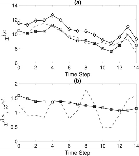
For this realization, the time average of the squared analysis errors for the RKFbc and the SKFbc are the same to two decimal places. However, the SKFbc does have a smaller true large-scale analysis error variance than the RKFbc and the difference increases more as ${\mathrm{C}}^{\delta }$ is more optimally chosen. The same is true for the RKF and SKF with modelled variance ${\mathrm{C}}^s.$

In Fig. 5b we see the bias value estimated by the SKFbc and the small-scale true model solution for a particular realization, which is dominated by noise. The bias state $x_k^{\beta ,a}$ is intended to estimate the expected value of the small-scale state evolved with the filter forecast model such that it is unaffected by small-scale noise (see (7.3)(7.3) $${\mathit{x}}^s={\mathit{x}}^{\beta }+{\mathit{x}}^{\delta },$$(7.3) ). Using (2.2)(2.2) $${\left(\begin{array}{c}{\mathit{x}}^{l,t}\\ {\mathit{x}}^{s,t}\end{array}\right)}_k=\left(\begin{array}{cc}{\mathbf{M}}^l& {\mathbf{0}}_{N_l\times N_s}\\ {\mathbf{M}}^{sl}& {\mathbf{M}}^s\end{array}\right){\left(\begin{array}{c}{\mathit{x}}^{l,t}\\ {\mathit{x}}^{s,t}\end{array}\right)}_{k-1}-{\left(\begin{array}{c}{\mathit{\eta }}^l\\ {\mathit{\eta }}^s\end{array}\right)}_k.$$(2.2) we see that $〈{\mathit{x}}_k^{s,t}〉=〈{\mathbf{M}}^{sl}{\mathit{x}}_{k-1}^{l,t}+{\mathbf{M}}^s{\mathit{x}}_{k-1}^{s,t}+{\mathit{\eta }}_k^s〉$ where the angular brackets indicate the mathematical expectation over the distribution of the small-scale model errors. Here, we have plotted $x_k^{s,t}$ which is dependent on the large-scale noise and small-scale noise (cf. (2.2)(2.2) $${\left(\begin{array}{c}{\mathit{x}}^{l,t}\\ {\mathit{x}}^{s,t}\end{array}\right)}_k=\left(\begin{array}{cc}{\mathbf{M}}^l& {\mathbf{0}}_{N_l\times N_s}\\ {\mathbf{M}}^{sl}& {\mathbf{M}}^s\end{array}\right){\left(\begin{array}{c}{\mathit{x}}^{l,t}\\ {\mathit{x}}^{s,t}\end{array}\right)}_{k-1}-{\left(\begin{array}{c}{\mathit{\eta }}^l\\ {\mathit{\eta }}^s\end{array}\right)}_k.$$(2.2) ). From this panel we see that the bias estimate is consistent with the small-scale true model solution.

Additional experiments using persistence as the forecast model for the bias state with the SKFbc have been carried out. We find that the time average of the SKFbc squared analysis errors is approximately three times smaller than the time average of the SKF squared analysis errors without bias correction. Nevertheless, the mean-square analysis errors for the SKFbc with the persistence bias model are more than 50% larger than when using (7.2)(7.2) $${\mathit{x}}_k^{\beta }={\mathbf{M}}^{sl}{\mathit{x}}_{k-1}^l+{\mathbf{M}}^s{\mathit{x}}_{k-1}^{\beta },$$(7.2) . Additionally, when using persistence as the forecast model for the bias state in the RKFbc we find the time average of the squared analysis errors is also approximately three times less than the SKF error. Hence, for this system it is more important to treat the bias due to unresolved scales than compensate for the unbiased error due to unresolved scales.

9.2. Determining the optimal ${\mathrm{C}}^{\delta }$ over the assimilation window

In this section we determine the optimal ${\mathrm{C}}^{\delta }$ over the whole assimilation window.

For the SKF, we found that the choice of ${\mathrm{C}}^s$ was key to the performance of the filter. We follow a similar procedure to section 6.1 to find the optimal values of the unbiased small-scale error covariance ${\mathrm{C}}^{\delta }.$ Our experiments have an assimilation window of 15 time-steps with an observation assimilated at each time-step. To find the optimal ${\mathrm{C}}^{\delta }$ for given parameter values for ${\mathrm{R}}^I$ and ${\mathrm{Q}}^s,$ we calculate the true large-scale analysis error variance of the SKFbc for ${\mathrm{C}}^{\delta }$ ranging from 0 to 1 in steps of $\Delta {\mathrm{C}}^{\delta }=0.001$ and save the value that produces the smallest variance at the final time-step.

Figure 6 shows the optimal ${\mathrm{C}}^{\delta }$ for different values of ${\mathrm{Q}}^s$ and ${\mathrm{R}}^I.$ The behaviour is qualitatively similar to ${\mathrm{C}}^s$ with the SKF shown in Fig. 1 but numerical comparison is not meaningful as a different model is used. In particular, the size of ${\mathrm{C}}^{\delta }$ is primarily determined by the magnitude of ${\mathrm{Q}}^s.$ However, we find that an increase in ${\mathrm{R}}^I$ can also result in a larger ${\mathrm{C}}^{\delta }$ being optimal. If ${\mathrm{M}}^{sl}$ is increased, the optimal ${\mathrm{C}}^{\delta }$ decreases as the uncertainty caused by the contribution from the large-scale processes to the small-scale state becomes more important.

Fig. 6. The values of ${\mathrm{C}}^{\delta }$ which give the minimum true large-scale analysis error variance at the end of the assimilation window for the SKFbc.

9.3. Comparison of the bias correction filters

In this section we evaluate the performance of the SKFbc and RKFbc relative to the OKF and examine their perceived error variances.

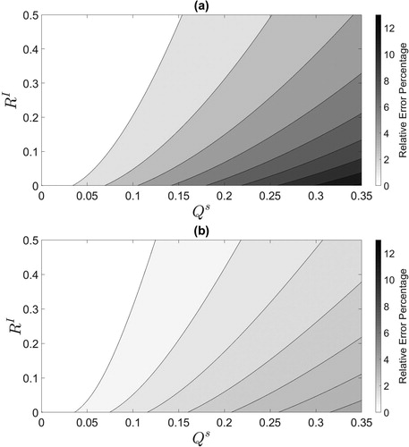
We now compare the SKFbc and RKFbc with the OKF in terms of relative error percentage (6.1)(6.1) $$\text{relative}\mathrm{ }\text{error}\mathrm{ }\text{percentage}=\frac{\left|{\tilde{\mathrm{P}}}_{\mathit{RKF}/\mathit{SKF}}^{ll,a}-{\tilde{\mathrm{P}}}_{\mathit{OKF}}^{ll,a}\right|}{{\tilde{\mathrm{P}}}_{\mathit{OKF}}^{ll,a}}\times 100\%,$$(6.1) , plotted in Fig. 7. The SKFbc provides most improvement over the RKFbc for large ${\mathrm{Q}}^s$ and small ${\mathrm{R}}^I.$ This behaviour is qualitatively similar to the comparison between the RKF and SKF with the OKF shown in Fig. 3. We have also examined the perceived and true analysis error variances for the RKFbc and SKFbc (not plotted). The results are qualitatively similar to those given in section 6.2 for the RKF and SKF. Indeed, for non-negligible representation uncertainty the SKFbc (RKFbc) is a conservative (overconfident) filtering strategy as the perceived-minus-truth difference is positive (negative).

Fig. 7. (a): Comparison of the RKFbc to the OKF in terms of relative error percentage given by equation (6.1)(6.1) $$\text{relative}\mathrm{ }\text{error}\mathrm{ }\text{percentage}=\frac{\left|{\tilde{\mathrm{P}}}_{\mathit{RKF}/\mathit{SKF}}^{ll,a}-{\tilde{\mathrm{P}}}_{\mathit{OKF}}^{ll,a}\right|}{{\tilde{\mathrm{P}}}_{\mathit{OKF}}^{ll,a}}\times 100\%,$$(6.1) . (b): Comparison of the SKFbc with optimal ${\mathrm{C}}^{\delta }$ to the OKF at the final time-step in terms of relative error percentage.

10. Summary and conclusion

Observations of the atmospheric state may contain information on spatio-temporal scales unable to be represented by a numerical model. The resulting error caused by this scale mismatch between the observations and numerical model is known as the error due to unresolved scales. To obtain accurate analyses from assimilation of these observations requires that the data assimilation algorithm correctly account for this error.

In this work we have considered the ability of linear filters to compensate for the error due to unresolved scales. We considered a finite dimensional true state which could be partitioned into a large-scale state resolved by a numerical model and a small-scale state unresolved by a numerical model. The representation error was defined in this framework and a bias due to unresolved scales was shown to occur when there is a contribution from the large-scale processes to the small-scale state.

For our experiments we considered three filters: the Schmidt-Kalman filter (Janjić and Cohn, 2006) that analyses the large-scales but models the uncertainty on all scales; the optimal Kalman filter, which analyses all scales, and a reduced-state Kalman filter, which completely disregards the small-scale processes.

The three filters were tested numerically on a random walk model with one variable for the large-scale processes and one variable for the small-scale processes. The observations were taken to be the sum of the large- and small-scale states with added noise to simulate instrument error. To obtain the best performance from the Schmidt-Kalman filter we had to tune the modelled small-scale error covariance to compensate for the variability of the small-scale processes which grew over the first half of the assimilation window. The Schmidt-Kalman filter works best in regimes of high error due to unresolved scales and low instrument error provided a suitable approximate small-scale error covariance is used. Examination of the perceived error variances revealed the analysis uncertainty calculated by the Schmidt-Kalman filter is greater than the true analysis uncertainty when accounting for error due to unresolved scales.

The novel use of the Schmidt-Kalman filter with an observation bias correction scheme was introduced as a means to correct the bias due to unresolved scales. The Schmidt-Kalman filter with a bias correction scheme proved to be a suitable method to treat observation biases and compensate for due to unresolved scales. In our experiments we found it was more important to treat an observation bias than to compensate for an unbiased error due to unresolved scales.

An important note to make regarding these experiments was that we had complete knowledge of the small-scale processes. This allowed for minimal approximations to be made to implement the Schmidt-Kalman filter and to tune the modelled error variances. In an operational setting, where all the small-scale processes are likely to be unknown, further approximations would be required. Additionally, the Schmidt-Kalman filter is a computationally expensive method due to the augmentation and propagation of the state error covariances. This must also be addressed before the filter could be considered for large problems.

Disclosure statement

No potential conflict of interest was reported by the authors.

Additional information

Funding

Z.

Bell was supported by a University of Reading PhD studentship. S. L. Dance and J. A. Waller were supported in part by UK EPSRC grant EP/P002331/1 (DARE). We would also like to thank two anonymous referees whose comments have helped improve the quality of this paper.

References

- Aravéquia, J. A., Szunyogh, I., Fertig, E. J., Kalnay, E., Kuhl, D. and co-authors. 2011. Evaluation of a strategy for the assimilation of satellite radiance observations with the local ensemble transform Kalman filter. Mon. Weather Rev. 139, 1932–1951. doi:10.1175/2010MWR3515.1
- Asher, R. B., Herring, K. D. and Ryles, J. C. 1976. Bias, variance, and estimation error in reduced order filters. Automatica 12, 589–600. doi:10.1016/0005-1098(76)90040-6
- Asher, R. B. and Reeves, R. M. 1975. Performance evaluation of suboptimal filters. IEEE Trans. Aerosp. Electron. Syst. AES-11, 400–405. doi:10.1109/TAES.1975.308092
- Brown, R. G. and Hwang, P. Y. 2012. Introduction to Random Signals and Applied Kalman Filtering. John Wiley & Sons, Hoboken, NJ, p. 192, Chapter 5.
- Brown, R. and Sage, A. 1971. Analysis of modeling and bias errors in discrete-time state estimation. IEEE Trans. Aerosp. Electron. Syst. AES-7, 340–354. doi:10.1109/TAES.1971.310375
- Cordoba, M., Dance, S. L., Kelly, G. A., Nichols, N. K. and Waller, J. A. 2017. Diagnosing atmospheric motion vector observation errors for an operational high-resolution data assimilation system. Q. Meteorol. Soc. 143, 333–341. doi:10.1002/qj.2925
- Daley, R. 1993. Estimating observation error statistics for atmospheric data assimilation. Ann. Geophysicae 11, 634–647.
- Dee, D. P. 2005. Bias and data assimilation. Q. J. R. Meteorol. Soc. 131, 3323–3343. doi:10.1256/qj.05.137
- Dee, D. 2004. Variational bias correction of radiance data in the ECMWF system. In: Proceedings of the ECMWF Workshop on Assimilation of High Spectral Resolution Sounders in NWP, Reading, UK, ECMWF.
- Derber, J. C. and Wu, W.-S. 1998. The use of TOVS cloud-cleared radiances in the NCEP SSI analysis system. Mon. Wea. Rev. 126, 2287–2299. doi:10.1175/1520-0493(1998)126<2287:TUOTCC>2.0.CO;2
- Desroziers, G., Berre, L., Chapnik, B. and Poli, P. 2005. Diagnosis of observation, background and analysis-error statistics in observation space. Q. J. R. Meteorol. Soc. 131, 3385–3396. doi:10.1256/qj.05.108
- Eyre, J. 2016. Observation bias correction schemes in data assimilation systems: a theoretical study of some of their properties. Q. J. R. Meteorol. Soc. 142, 2284–2291. doi:10.1002/qj.2819
- Fertig, E., Baek, S.-J., Hunt, B., Ott, E., Szunyogh, I. and co-authors. 2009. Observation bias correction with an ensemble Kalman filter. Tellus A: Dyn. Meteorol. Oceanogr. 61, 210–226. doi:10.1111/j.1600-0870.2008.00378.x
- Fielding, M. and Stiller, O. 2019. Characterizing the representativity error of cloud profiling observations for data assimilation. J. Geophys. Res. Atmos. 124, 4086–4103. doi:10.1029/2018JD029949
- Friedland, B. 1969. Treatment of bias in recursive filtering. IEEE Trans. Automat. Contr. 14, 359–367. doi:10.1109/TAC.1969.1099223
- Gelb, A. 1974. Applied Optimal Estimation. MIT Press, Cambridge, MA, and London, UK, Chapter 8, pp. 305–306.
- Grooms, I., Lee, Y. and Majda, A. J. 2014. Ensemble Kalman filters for dynamical systems with unresolved turbulence. Comput. Phys. 273, 435–452. doi:10.1016/j.jcp.2014.05.037
- Hodyss, D. and Satterfield, E. 2016. Mathematical concepts of data assimilation. In: Data Assimilation for Atmospheric, Oceanic and Hydrologic Applications (eds. S. K. Park and L. Xu) Vol. 3. Springer, Berlin, pp. 177–194.
- Ignagni, M. 1981. An alternate derivation and extension of Friendland’s two-stage Kalman estimator. IEEE Trans. Automat. Contr. 26, 746–750. doi:10.1109/TAC.1981.1102697
- Janjić, T., Bormann, N., Bocquet, M., Carton, J., Cohn, S. and co-authors. 2018. On the representation error in data assimilation. Q. J. R. Meteorol. Soc. 144, 1257–1278. doi:10.1002/qj.3130
- Janjić, T. and Cohn, S. E. 2006. Treatment of observation error due to unresolved scales in atmospheric data assimilation. Mon. Weather Rev. 134, 2900–2915. doi:10.1175/MWR3229.1
- Jazwinski, A. H. 1970. Stochastic Processes and Filtering Theory. Academic Press, New York, NY, Chapter 7, p. 212.
- Kalman, R. E. 1960. A new approach to linear filtering and prediction problems. Journal of Basic Engineering 82, 35–45. doi:10.1115/1.3662552
- Karspeck, A. R. 2016. An ensemble approach for the estimation of observational error illustrated for a nominal 1° global ocean model. Mon. Wea. Rev. 144, 1713–1728. doi:10.1175/MWR-D-14-00336.1
- Lea, D., Drecourt, J.-P., Haines, K. and Martin, M. 2008. Ocean altimeter assimilation with observational-and model-bias correction. Q. J. R. Meteorol. Soc. 134, 1761–1774. doi:10.1002/qj.320
- Liu, Z.-Q. and Rabier, F. 2002. The interaction between model resolution, observation resolution and observation density in data assimilation: A one-dimensional study. Q J. R Meteorol. Soc. 128, 1367–1386. doi:10.1256/003590002320373337
- Ménard, R. 2010. Bias estimation. In: Data Assimilation: making Sense of Observations (eds. W. Lahoz, B. Khattatov and R. Menard). Springer, Berlin, pp. 113–135.
- Miyoshi, T., Sato, Y. and Kadowaki, T. 2010. Ensemble Kalman filter and 4D-Var intercomparison with the Japanese operational global analysis and prediction system. Mon. Weather Rev. 138, 2846–2866. doi:10.1175/2010MWR3209.1
- Moodey, A. J. 2013. Instability and regularization for data assimilation. PhD thesis, University of Reading.
- Nichols, N. 2010. Mathematical concepts of data assimilation. In: Data Assimilation: making Sense of Observations (eds. W. Lahoz, B. Khattatov and R. Menard). Springer, Berlin, pp. 13–39.
- Oke, P. R. and Sakov, P. 2008. Representation error of oceanic observations for data assimilation. J. Atmos. Oceanic Technol. 25, 1004–1017. doi:10.1175/2007JTECHO558.1
- Satterfield, E., Hodyss, D., Kuhl, D. D. and Bishop, C. H. 2017. Investigating the use of ensemble variance to predict observation error of representation. Mon. Weather Rev. 145, 653–667. doi:10.1175/MWR-D-16-0299.1
- Schmidt, S. F. 1966. Application of state-space methods to navigation problems. In: Advances in Control Systems (ed. C. T. Leondes) Vol. 3. Elsevier, Amsterdam, pp. 293–340.
- Schutgens, N. A., Gryspeerdt, E., Weigum, N., Tsyro, S., Goto, D. and co-authors. 2016. Will a perfect model agree with perfect observations? The impact of spatial sampling. Atmos. Chem. Phys. 16, 6335–6353. doi:10.5194/acp-16-6335-2016
- Simon, D. 2006. Optimal State Estimation: Kalman, H Infinity, and Nonlinear Approaches. Wiley-Blackwell, Hoboken, NJ, pp. 309–312, Chapter 10.
- Stewart, L. M., Dance, S. L., Nichols, N. K., Eyre, J. R. and Cameron, J. 2014. Estimating interchannel observation-error correlations for IASI radiance data in the Met Office system. Q. J. R. Meteorol. Soc. 140, 1236–1244. doi:10.1002/qj.2211
- Todling, R. and Cohn, S. E. 1994. Suboptimal schemes for atmospheric data assimilation based on the Kalman filter. Mon. Wea. Rev. 122, 2530–2557. doi:10.1175/1520-0493(1994)122<2530:SSFADA>2.0.CO;2
- Waller, J. A., Ballard, S. P., Dance, S. L., Kelly, G., Nichols, N. K. and co-authors. 2016a. Diagnosing horizontal and inter-channel observation error correlations for SEVIRI observations using observation-minus-background and observation-minus-analysis statistics. Remote Sens. 8, 581. doi:10.3390/rs8070581
- Waller, J. A., Dance, S. L., Lawless, A. S., Nichols, N. K. and Eyre, J. 2014. Representativity error for temperature and humidity using the Met Office high-resolution model. Q. J. R. Meteorol. Soc. 140, 1189–1197. doi:10.1002/qj.2207
- Waller, J. A., Simonin, D., Dance, S. L., Nichols, N. K. and Ballard, S. P. 2016b. Diagnosing observation error correlations for Doppler radar radial winds in the Met Office UKV model using observation-minus-background and observation-minus-analysis statistics. Mon. Wea. Rev. 144, 3533–3551. doi:10.1175/MWR-D-15-0340.1
- Zhu, Y., Derber, J., Collard, A., Dee, D., Treadon, R. and co-authors. 2014. Enhanced radiance bias correction in the National Centers for Environmental Prediction’s gridpoint statistical interpolation data assimilation system. Q. J. R. Meteorol. Soc. 140, 1479–1492. doi:10.1002/qj.2233