Adding CO₂ channel 16 to AHI data assimilation over land further improves short-range rainfall forecasts

Abstract

The new generation of geostationary environmental operational satellite imager, the Himawari-8 Advanced Himawari Imager (AHI), adds two more water vapour channels and four more other channels than its predecessor, MTSAT-2. But except for the three water vapour channels, AHI channels are often not assimilated over land due to large uncertainty in surface parameters. Using the relative adjoint sensitivity analysis method, we show that the brightness temperature of AHI channel 16 is much more sensitive to the low-tropospheric atmosphere than to the surface emissivity, similar to those high-level water vapour channels. We thus assimilated AHI channel 16 brightness temperature observations together with AHI water vapour channels over land, and assessed the added benefits on short-range quantitative precipitation forecasts for several convection-induced rainfall cases. Results show that adding channel 16 over land to AHI data assimilation further improves short-range rainfall forecasts. Assimilation of AHI channel 16 improves the upstream near surface atmospheric temperature analysis and influences the development of downstream precipitating weather systems.

Keywords:

• data assimilation
• geostationary satellite
• AHI
• land

1. Introduction

Accurate initial conditions are important for obtaining accurate numerical weather forecasts. With the growing demand for numerical weather forecasts and the increasing variety of meteorological observation means, more and more observations are incorporated into data assimilation systems to produce accurate initial conditions of numerical weather forecasting models. Among many types of meteorological observations, satellite observations already become the absolute majority, accounting for about 98% of meteorological observations (Kelly and Thepaut, 2007). Therefore, the potential for satellite observation assimilation is especially important for the above purposes.

In the 1990s, direct assimilation of satellite radiance observations in the framework of variational data assimilation brought the applications of satellite data in numerical weather prediction into a new era (Eyre et al., 1993). Many studies have proved that the direct assimilation of satellite radiance observations significantly improved numerical weather prediction (Andersson et al., 1994; Derber and Wu, 1998; English et al., 2000; Bouttier and Kelly, 2001; Eyre, 2007; Fertig et al., 2009; Miyoshi et al., 2010). Meteorological satellites mainly move in either polar-orbiting or geostationary tracks. Polar-orbiting operational environmental satellite observations have global coverage and various microwave and infra-red spectral bands, have been assimilated in operational data assimilation systems globally for nearly a decade earlier than observations of geostationary satellites. However, with improvement in both the spectral resolution of observations of geostationary satellites and the spatial resolution of numerical weather prediction models, more attention has been paid to assimilating geostationary satellites data, which have high spatial and temporal resolutions. Although the spectral resolution of imagers of geostationary satellites is usually lower than remote-sensing instruments onboard on polar orbit satellites, their high spatial and temporal resolutions provide more abundant observation information about mesoscale and convective scale weather systems. The launch of the new generation of geostationary satellites from Japan, the United States and China has further promoted the data assimilation research of geostationary satellites. Following the successful launches of Meteosat Second Generation (MSG) developed by the European Space Agency (ESA) and by European Organisation for the Exploitation of Meteorological Satellites (EUMETSAT) carrying the Spinning Enhanced Visible and Infrared Imager (SEVIRI) (Schmetz et al., 2002), Japan Himawari-8/9 carrying the Advanced Himawari Imager (AHI) (Bessho et al., 2016), the GOES-R (The Geostationary Operational Environmental Satellite-R Series) of the United States carrying the Advanced baseline imager (ABI) (Schmit et al., 2017), China FY-4A (Feng-Yun-4A) carrying the Advanced Geostationary Radiation Imager (AGRI) (Yang et al., 2017) and Korean GEO-KOMPSAT-2A carrying the Advanced Meteorological Imager (AMI) (Choi and Ho, 2015), assimilation of infra-red channels from these geostationary satellites imagers has played and will continue to play a significant role for improving the numerical weather prediction skill.

Scientists assessed the impacts of assimilating infra-red channels of geostationary satellites imagers in the global (Köpken et al., 2004; Szyndel et al., 2005; Ma et al., 2017) and regional (Montmerle et al., 2007; Stengel et al., 2009; Zou et al., 2011; Qin et al, 2013, 2017; Qin and Zou, 2018) weather forecasting systems. Improvements on numerical forecasts of high impact weathers such as typhoons were demonstrated by Zou et al. (2015), Zhang et al. (2016), Minamide and Zhang (2018), Honda, Miyoshi et al. (2018) and Honda, Kotsuki et al. (2018). At present, imagers infra-red channels of geostationary satellites have been successfully assimilated in the operational data assimilation system of NCEP (Derber, 2003), the Canadian data assimilation system (Garand and Wagneur, 2002) and the ECMWF (European Center for Medium Range Weather Forecast) (Köpken et al., 2003; Szyndel et al., 2005). The new generation of imagers AHI and ABI have already been assimilated by the operational data assimilation systems in Japan (Kazumori, 2016) and United States (Ma et al., 2017).

Most of data assimilation researches of geostationary satellites focussed on water-vapour sounding channels, such as channel 2 (6.2 µm) and channel 3 (7.3 µm) of SEVIRI, which was carried on the geostationary satellite Meteosat-8 in the early stage (Montmerle et al., 2007; Kelly, 2008). Zhang et al. (2016) and Jones et al. (2018) assimilated the GOES-13/15 infra-red channel 3 (6.5 µm). Only the AHI water-vapour channel 9 was assimilated in Honda, Miyoshi et al. (2018) and Honda, Kotsuki et al. (2018). Zhang et al. (2018) assimilated the ABI channel 10, while and Zhang et al. (2016), Ma et al. (2017) and Wang et al. (2018) assimilated all three AHI or ABI water-vapour sounding channels 8, 9 and 10. Stengel et al. (2013) improved cloudy radiance data assimilation of SEVIRI by introducing a simplified cloud diagnosis algorithm, Zhang et al. (2016), Honda, Miyoshi et al. (2018) and Honda, Kotsuki et al. (2018) included cloudy data in the assimilation by adjusting observation errors adaptively.

There were studies on assimilation of other imager infra-red channels besides those water vapour channels over the oceans. Stengel et al. (2009, 2010) assimilated the data of 13.4 µm channel of SEVIRI over the ocean, and Qin et al. (2017) and Qin and Zou (2018) assimilated all surface-sensitive infra-red channels of AHI and ABI over oceans. The assimilation of surface-sensitive channels over land faces many difficulties due to large uncertainty in the descriptions of land surface emissivity and land surface temperature (Guedj et al., 2011). By introducing a satellite-based surface temperature retrieval method, Guedj et al. (2011) made an effort to assimilate the three infra-red surface-sensitive channels (8.7, 12.0 and 13.4 µm) of SEVIRI. Although some improvements were obtained for precipitation forecasts in the southern Europe, daily and seasonal variations of the surface temperature retrieval accuracy, the reuse of background information, and the dependence on the accuracy of surface emissivity data set remain to be challenging problems (Zheng et al., 2009).

This study explores a possibility of assimilating some AHI surface-sensitive channels over land, in addition to the three AHI water-vapour sounding channels. An adjoint relative sensitivity study shows that the brightness temperatures of AHI channel 16 (13.3 µm) are more sensitive to the atmospheric temperature in the lower troposphere than to the land surface emissivity, suggesting a possibility to include channel 16 in AHI data assimilation over land. Section 2 provides a brief description of AHI data characteristics and experiment design. Section 3 presents some statistical results on the differences between AHI observations and simulations over land and ocean. Using an adjoint sensitivity analysis method, section 4 discusses the relative sensitivity of AHI brightness temperatures at different channels to atmospheric temperature, water vapour and surface emissivity. The impacts of the assimilation of all AHI infra-red channels over ocean and only AHI water-vapour sounding channels 8–10 and CO₂ channel 16 over land are presented in section 5. Summary and conclusions are given in section 6.

2. Data and case descriptions

AHI is an imager instrument onboard the Japanese geostationary satellite Himawari-8, which was successfully launched by the Meteorological Satellite Center (MSC) of the Japan Meteorological Agency (JMA) on 7 October 2014 and officially put into operation on 7 July 2015. AHI is able to observe a range of 120 degrees longitude and latitude from the equatorial centre position at 140°E. It has 16 channels, including three visible light channels, three near-infra-red channels and 10 infra-red channels. The specific frequency information can be found in (Bessho et al., 2016). The 10 infra-red channels are employed for AHI data assimilation. Channels 8, 9 and 10 are water vapour sounding channels, with frequencies centred at 6.2, 6.9 and 7.3 µm, respectively. The weight functions of channels 8, 9 and 10 peak at about 377, 457 and 587 hPa, respectively. The weight functions of other seven infra-red channels peak at the surface (see Fig. 1 in Zou et al., 2016). The centre frequencies of channels 7, 11–16 are located at 3.85, 8.60, 9.63, 10.45, 11.20 12.35 and 13.3 μm, respectively. Channel 12 is an ozone sensitive channel and its weighting function has a second peak in the stratosphere. The AHI channel 16 is located within a wing of a strong CO₂ absorption band.

Fig. 1. Spatial distributions of the 24-h accumulative rainfall observations and geopotential height at 500 hPa (a) from 0000 UTC July 1 to 0000 UTC July 2 (case 1), (b) from 0000 UTC July 10 to 0000 UTC July 11 (case 2), and (c) from 1200 UTC July 19 to 1200 UTC July 20, 2016 (case 3).

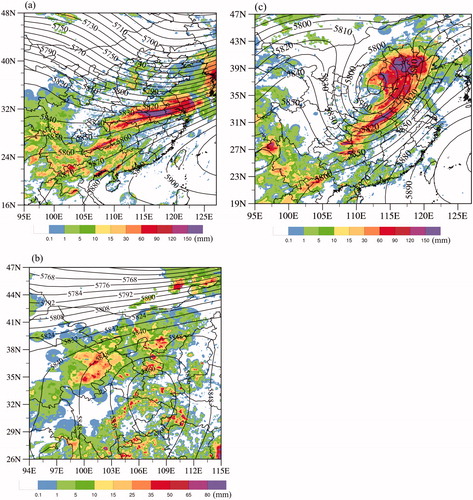
Three precipitation cases that occurred in July 2016 were selected for this study. Case 1 is a heavy rainfall process that occurred during the period from 0000 UTC 1 July to 0000 UTC 2 July 2016 in the middle and lower reaches of the Yangtze River in Hubei, Anhui and Jiangsu provinces in the central China. Case 2 is a weak precipitation event that occurred in Qinghai, Inner Mongolia and Gansu Province in Northwest China from 0000 UTC 10 July 2016 to 0000 UTC 11 July 2016. Case 3 is a strong precipitation process that occurred in Shandong, Shanxi, Hebei, Beijing and Tianjin areas in the northern China from 1200 UTC 19 July 2016 to 1200 UTC 20 July 2016.

Figure 1 shows the spatial distributions of 24-hour accumulated precipitation observations of the above three precipitation cases during the 24-h model forecasting periods, as well as the geopotential height at 500 hPa of FNL (Final Operational Global Analysis) data produced by the Global Data Assimilation System (GDAS) of American NCEP (National Center for Environmental Prediction) in the middle of the three 24-hour periods, i.e. 1200 UTC 1 July, 1200 UTC 10 July and 0000 UTC 20 July 2016. The rainfall observations were obtained from merging hourly rain gauge data at more than 30,000 automatic weather stations in China with the Climate Precipitation Center Morphing (CMORPH) precipitation product using a probability-density-function-based optimal interpolation method (Shen et al. 2014). The case-1 precipitation event was associated with a middle latitude trough and a subtropical high. The cold air from the north brought by the airflow in the back of the trough and the warm wet air advected from the northwest under the influence of the subtropical high met in the Yangtze River Basin where precipitation occurred. Because of a stable maintenance of the subtropical high and the slow eastward movement of the trough, the rainfall in the Yangtze River Basin was quite heavy. The case-2 precipitation distribution was of a small-scale nature and was associated a vortex convective system seen at 500 hPa. The precipitation is located in Qinghai, Inner Mongolia and Ningxia, and some sporadic precipitations occurred in Sichuan and Hubei in the south of the vortex. In case 3, the precipitation is mainly caused by the deep frontal cyclone in the westerly, to its southeast that was a subtropical high. The cyclone moved eastward and the subtropical high stretches northwestward, bringing warm, moist airs into Beijing, Tianjin and Hebei. A heavy rainfall event occurred in Shandong, Shanxi and Henan areas.

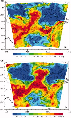
The WRF-ARW (Weather Research and Forecasting/Advanced Research WRF) model and the Gridpoint Spectral Interpolation (GSI) data assimilation system (Shao et al., 2016) are selected in this study. Figure 2 shows the model domain. The horizontal resolution is 6 km, with total model grid points of 600 × 600. The model top is set to 1 hPa, with a total of 61 vertical layers. The WRF single-moment three-class microphysics scheme (Hong and Lim, 2006), and the Yonsei planetary boundary layer scheme (Hong and Dudhia, 2003) are used in the WRF-ARW model. Also shown in Fig. 2 are the spatial distributions of geopotential height and relative humidity at 500 hPa at the starting and ending time of the 24-h data assimilation cycling period of case 3. Seen in this figure is a middle latitude trough intensified during the 24 hours. A high relative humidity band is located ahead of the trough.

Fig. 2. Spatial distributions of 500-hPa geopotential height from the NCEP reanalysis (black curve, contour interval: 20 m) and relative humidity (color shading, unit: %) in the model domain at (a) 1200 UTC 18 July (beginning time of the DA cycling for case 3) and (b) 1200 UTC 19 July (ending time of the DA cycling for case 3), 2016.

GSIV3.3 is used as the data assimilation system in our study, which is a three-dimensional variational assimilation system, which can be well applied to global and regional data assimilation research. The system can well assimilate conventional observation data, radar data, microwave and infra-red radiance data of main polar orbiting satellites, as well as infra-red imagers of geostationary satellites. The system also provides an adjustable background error covariance matrix and a correction scheme of observation error and deviation, which can be adjusted adaptively for specific regions. In the GSI, the background error covariance was constructed using recursive filters (Wu et al., 2002). It is an inhomogeneous and anistrophic background error covariance matrix of streamfunction, unbalanced part of velocity potential, unbalanced part of temperature, unbalanced part of surface pressure, and normalised relative humidity. The fast radiative transfer model used is the community radiative transfer model (CRTM) v2.1.3 (Han et al., 2007). The quality control is carried out based on some parameters associated with cloud, water vapour, and temperatures, surface emissivity, and observation errors, which was described in details by Zou et al. (2013). Bias correction consists of a static bias correction and an air mass bias correction (Zhu et al., 2014; Li et al., 2019). Static scan biases specified by GSI are removed firstly. After that, the air mass bias correction scheme in the GSI is applied. Coefficients for air mass bias correction method are derived from one-month iterative data assimilation experiments. Other details of the GSI satellite data assimilation can be found in Shao et al. (2016).

3. O-B biases of AHI data

Over the land area, model simulations of AHI surface-sensitivity channels are usually much less accurate than the upper-level water vapour channels due to the uncertainty in the land surface emissivity and surface temperature. We may use the hourly AHI observations at 2 km resolution from July 1 to 31, 2016 to show the mean and standard deviations (SD) of the differences between AHI observations and the CRTM (Community Radiative Transfer Model) model simulations (Han et al., 2007).

Hourly forecasts of the WRF-ARW model are taken as the background to evaluate the observational error and bias characteristics of AHI data in ocean and land areas from July 1 to 31, 2016. In order to correspond with real experiments, only the 6–12 hours forecast of WRF-ARW model initialised by the global FNL data are used here.

Figure 3a shows the bias characteristics and observation error of AHI channel 7–11, 13–16 data over land and ocean. The bars in the figure represent the average value of O-B, and the curves represent the result of the SD. Water-vapour channel 9 has the largest positive bias, while surface channel 11 and channel 16 have the most obvious negative bias. This result is similar to that of Zou et al. (2016).

Fig. 3. (a) Mean (bars) and standard deviation (curves) of O-B for AHI channels 7–10 and 11–16 data over land (solid bars and open circles) and ocean (dashed bars and stars) calculated from all data from July 1 to 31, 2016 in the model domain. (b) Standard deviation of O-B varying with terrain height for AHI channels 7–10 and 11–16 calculated from all data from July 1 to 31, 2016 in the model domain.

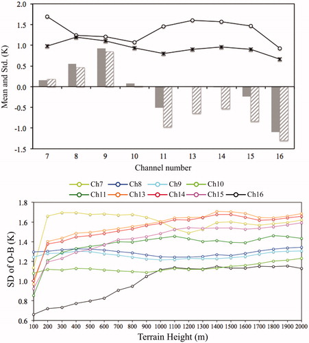
SD has significant differences between land and ocean for those surface channels. It can be seen that the SD of each channel over ocean (the asterisk curve) shows a good consistency, all around 1.0 K. However, the SD of those surface channels increased significantly over land (the hollow circle curve). The SD of channel 7, 11–15 all reached 1.5 K, but the SD of channel 16, which was more sensitive to CO₂, only increased slightly, showing similar characteristics with those water-vapour channels. It may represent that brightness temperature simulation of channel 16 is very little affected by land surface variables (Stengel et al., 2009).

The influence of terrain height on SD of O-B is shown in Fig. 4b. SDs of high-level channels are less affected by the terrain height. However, observation errors of those surface-sensitivity channels are significantly different with the change of terrain height. The observation error of channel 16 increases gradually with the terrain height when the terrain height is less than 1000 m, but for the terrain higher than 100 m, it remains at 1.1 K. For other surface-sensitivity channels, there is an obvious increase in observation errors at the height of 0–200 m, but they increase slowly after 200 m.

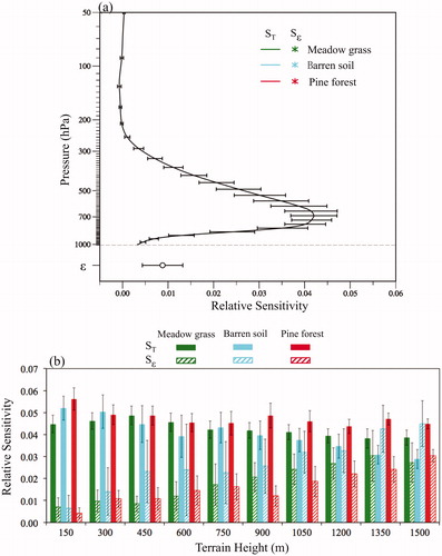
Fig. 4. (a) The mean (curve and open circle) and the one standard deviation (vertical line) of relative sensitivity of channel-16 brightness temperature to air temperature (curve) and surface emissivity (open circle) averaged for all data from July 1 to 31, 2016 in the model domain. (b) The mean (bars) and the one standard deviation (vertical lines) of maximum relative sensitivities of air temperature (solid bars) and surface emissivity (dashed bars) over meadow grass, barren soil and pine forest.

Since the peak of the weighting function of the CO₂ channel is located on the surface, most studies exclude the channel 16 in consideration of the large uncertainty of surface emissivity and surface temperature. From Statistical results of observation errors, we noticed that although the observation error of most surface-sensitivity channels over land will increase significantly, the increase of O-B of channel 16 is not obvious, which urges us to analyse this reason.

4. Relative sensitivity of AHI surface-sensitive channels

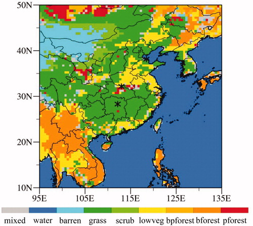
In order to further clarify the reason for the SD differences, we check the sensitivity of brightness temperature to surface variables over land. The most important factor affecting the surface emissivity is the surface types. CRTM includes a surface emissivity model, which can calculate the surface emissivity of each channel on the basis of given surface type. In order to facilitate the analysis of the impact of the surface types, the spatial distribution of the surface types given by Moderate Resolution Imaging Spectroradiometer (MODIS) land use developed by the International Geosphere–Biosphere Programme (IGBP) is also given in Fig. 5. It can be seen that the east of China is mainly characterised by a meadow grass surface, while the northwest region has mainly a bare soil surface. There are more pine forests and broad-leaved forests in the northeast, and irregular low vegetation in the middle of China. The grey areas in Fig. 5 represent a mixed surface type. Asterisks show the spatial locations of three selected data points used below.

Fig. 5. Spatial distribution of the major surface types within 0.5 × 0.5 horizontal grid boxes (>50%) from NPOESS dataset, including water (blue), barren soil (barren, cyan), meadow grass (grass, green), grass shrub land (scrub, light green), irrigated low vegetation (lwbeg, yellow), boardleaf pine forest (bpforest, light orange), boardleaf forest (bforest, orange), pine forest (pforest, red), and mixed (grey, not a single surface exceeds 50%). Asterisks show the spatial locations of three selected data points used below.

The sensitivity of brightness temperature to revelant variables can be evaluated by sensitivity calculated by the adjoint of radiative transfer model, but the sensitivity of different variables cannot be directly compared because of the difference of their units. Therefore, the relative sensitivity analysis method is used to investigate the sensitivity differences of brightness temperatures between channel 16 and other surface-sensitive channels (Carrier et al., 2008; Qin and Zou, 2019).

The nonlinear radiative transfer model can be expressed as $$T_k^b=H_k\left(\mathbf{x}\right)$$ where H is the operator with the input vector $\mathbf{x}$ to produce $T_k^b$ (the brightness temperature at channel $k$_, then the adjoint of radiative transfer model can be expressed as $$\widehat{\mathbf{x}}=H_k^T\left(\mathbf{x}\right){\widehat{T}}_k^b$$ where $H_k^T$ is called the adjoint operator, ${\widehat{T}}_k^b$ is the adjoint variable of brightness temperature.

For a sensitivity of brightness temperature, if we define the response function as: $$R_k\left(\mathbf{x}\right)=T_k^b,$$ then $${\widehat{T}}_k^b=\frac{\partial R_k}{\partial T_k^b}=1$$

The adjoint operator of radiative transfer model is used to obtain the gradient of $R_k$ with respect to the input variable $\mathbf{x},$ so the result after applying the adjoint is the gradient $\widehat{\mathbf{x}}.$ $$\widehat{\mathbf{x}}={\nabla }_x{R}_k$$ $R_k^{\mathit{sens}}$ is the sensitivity of the brightness temperature with respect to the input vector $\mathbf{x},$ it can be calculated by the following equation: $$R_k^{\mathit{sens}}={\left({\nabla }_x{\mathrm{R}}_k\right)}^T\delta x={\left(\widehat{x}\right)}^{\mathit{T}}\delta x$$ where $R_k^{}$ is the response function, it is simply defined as brightness temperature, $k$ is channel number, $\widehat{\mathbf{x}}$ is the gradient of the response function $R_k$ with respect to the input variable $\mathbf{x},$ $\delta x$ is the perturbation of the input variable.

The non-dimensional relative sensitivity $s_k^l$ to the variable l can be calculated as follows: $$s_k^l=\frac{R_k^{\mathit{sens},l}}{R_k}{\left(\frac{\delta x^l}{x^l}\right)}^{-1}\equiv \frac{{\widehat{x}}^l{x}^l}{R_k}$$

Figure 6a shows the temperature and specific humidity profiles at three arbitrarily selected data points over a bare soil, a pine forest and a meadow grass surface, respectively. The spatial locations of the three selected data points are indicated in Fig. 5. The terrain heights of bare soil, grassland and pine forest are 0.6, 118.3 and 3.4 m, respectively. Surface emissivities are 0.96, 0.94 and 0.99, respectively. The lowest atmospheric pressure is 1000.26, 992.0 and 974.60 hPa, respectively.

Fig. 6. (a) Vertical profiles of air temperature (solid curve) and specific humidity (dashed curve) and (b) relative sensitivity of channel-16 brightness temperature to air temperature (solid curve) and surface emissivity (stars) for the three land data points indicated in Fig. 5a (i.e. meadow grass, green; barren soil, cyan; and pine forest, red) at 1200 UTC 18 July 2016. Surface temperature at the meadow grass, barren soil, and pine forest points is 301.8, 300.19 and 303.26 K, respectively.

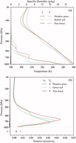
The relative sensitivity results of the channel-16 brightness temperatures to atmospheric temperature and land surface emissivity at these three data points of different surface types are provided in Fig. 6b. We find that the relative sensitivity of the channel-16 brightness temperature to atmospheric temperature is about an order of magnitude larger than that to the land surface emissivity. The peak relative sensitivity of the channel-16 brightness temperature to atmospheric temperature ranges from 0.0425 to 0.054, and the relatively sensitivity to the surface emissivity varies from 0.0025 to 0.007. The largest relative sensitivity is located at the 746-, 666, and 619-hPa pressure levels at the meadow grass, bare soil and pine forest points, respectively. Such results of the relative sensitivity of the channel-16 brightness temperature are significantly different from those of channels 11–15 (Fig. 7). The relative sensitivity of the channels 11–15 brightness temperatures to the surface emissivity is either larger than or similar to their sensitivity to the atmospheric temperatures.

Fig. 7. Same as Fig. 6b except for (a) AHI channel 11 (solid curve and star) and 12 (dashed curve and open circle), (b) channel 13 (solid curve and star) and 14 (dashed curve and open circle).

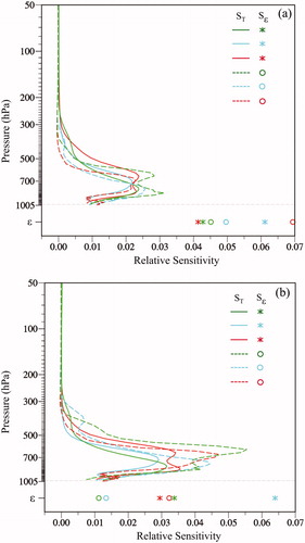
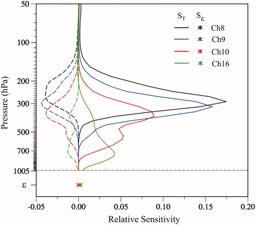
For completeness, we may compare the relative sensitivities of brightness temperatures among channels 8–10 and 16 at the meadow grass point (Fig. 8). The largest relative sensitivity to the atmospheric temperature is located at the 290-, 317, 376 and 746-hPa pressure levels, and the largest relative sensitivity to the specific humidity is located at the 264-, 290-, 346- and 690-hPa pressure levels for channels 8, 9, 10 and 16, respectively. The relative sensitivities to atmospheric temperature and specific humidity around these peak pressure levels are much higher than the relative sensitivities to the surface emissivity.

Fig. 8. Relative sensitivities of brightness temperatures for AHI channels 8 (green), 9 (blue), 10 (red) and 16 (black) to air temperature (solid curve), specific humidity (dashed curve) and surface emissivity (star) at 1200 UTC 18 July 2016 at (a) the pine forest point and (b) the broadleaf point indicated in Fig. 5a.

The mean and standard deviations of the relative sensitivities of the channel-16 brightness temperature simulation for all AHI data from July 1 to 31, 2016 to the temperature and surface emissivity in the entire model domain are provided in Fig. 4a. Figure 4b shows the impact of terrain height on the maximum relative sensitivity of atmospheric temperature and the relative sensitivity of surface emissivity for AHI channel 16. It can be seen that even if the relative sensitivity of surface emissivity increases with the terrain height, but it is still less than the maximum relative sensitivity of atmospheric temperature except for data over bare soil area with terrain higher than 1200 m.

It is thus of interest to examine if further improvements can be obtained by adding channel 16 to AHI data assimilation over land.

5. Impacts of AHI data assimilation on analyses and forecasts

In order to assess the impact of AHI data assimilation on the 24-h model forecasts, AHI data are assimilated together with conventional observations. Three data assimilation experiments are carried out for each case. The first is conventional data only experiment (CONV). The second experiment assimilates conventional data and AHI channel 8–10 data (E3CH). The third experiment is the same as the E3CH except for adding AHI channel 16 (E4CH). Each experiment starts with the 6-hour forecast initialised with the FNL analysis data 6 hours before the beginning of data assimilation cycling. The period of assimilation is 1 day, there are total 5 assimilations over a 6-hour window. For example, for case 1, assimilation is performed at 0000, 0600, 1200, 1800 UTC 1 July and 0000 UTC 2 July 2016, respectively, and then the 24-hour forecast is carried out.

The conventional observations are composed of a global set of surface and upper air reports operationally collected by NCEP. Only clear-sky AHI data are assimilated in E3CH and E4CH. Cloudy data are removed by using the infrared-only cloud detection method developed by Zhuge and Zou (2016). The newly calculated bias in Fig. 3a will be removed before data assimilation, the airmass bias correction method is then applied after the static bias correction. Observation errors for assimilated channels are also specified according to Fig. 3a. There is no additional consideration for the channel correlation of AHI data. In order to reduce a potential impact of spatial correlations of observation errors, the 2-km AHI observations are thinned to 60 km for both E3CH and E4CH. A 60-km equidistant grid is built by the GSI within the model domain, and AHI data closest to any of grid centres will be selected.

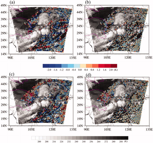
We may use case 3 as an example to compare analysis fields among three data assimilation experiments. Figure 9 shows the spatial distribution of the O-B and O-A of AHI channels 10 and 16 at the analysis time 0000 UTC July 19, 2016. The brightness temperature observations of AHI channel 14 (11.2 μm) are shown in a black/white shading to provide a general idea of cloud distribution at this time. It can be seen that only clear-sky data are assimilated. By comparing O-B and O-A fields, we can see that AHI data assimilation has a reasonably good convergence. The absolute values of O-A are consistently lower than those of O-B.

Fig. 9. Spatial distributions of O-B (left panels) and O-A (right panels) for (a)-(b) AHI channel 10 and (c)-(d) channel 16 at 0000 UTC 19 July 2016 for the experiment E4CH. Black dots represent data rejected by quality control. Black and white shaded represents the brightness temperature of AHI channel 14. The Magenta line shows the Tibet Plateau.

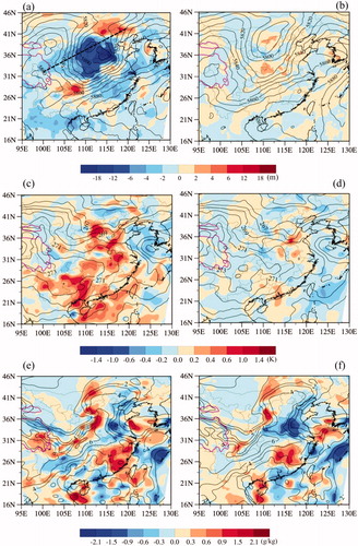
Figure 10 shows the spatial distributions of the geopotential height (Fig. 10a-b), air temperature (Fig. 10c-d) and specific humidity (Fig. 10e-f) analysis fields at 500 hPa and 0600 UTC 19 July 2016, as well as the analysis differences between E4CH and CONV (Fig. 10a, c, e) and those between the E3CH and the CONV (Fig. 10b, d, f). The 500-hPa geopotential field is characterised by a middle latitude cyclone system. The temperature trough lags behind the geopotential height trough, and the specific humidity in the trough area is significantly higher than in the surrounding areas. The cyclone in the E4CH is significantly deeper than that in the E3CH. The geopotential height in the E4CH trough region is more than −18 m lower than CONV (Fig. 10a). The temperature analysis from the E4CH is overall warmer than the CONV analysis (Fig. 10c). Differences of both the geopotential height and temperature analysis between E3CH and CONV are small (Fig. 10b, d). The experiment E3CH only assimilates the three water-vapour channels, which contain information of both the water vapour and temperature in upper and middle troposphere. The AHI data assimilation produces large differences in the specific humidity analysis between E3CH and CONV experiments (Fig. 10f). A positive analysis difference of specific humidity is found downstream of the trough and a negative analysis difference is located to the north of the positive centre. Features in the analysis differences of specific humidity between E4CH and CONV (Fig. 10e) are similar to and slightly larger magnitude than those between E3CH and CONV.

Fig. 10. Spatial distributions of the 500-hPa (a)-(b) geopotential height, (c)-(d) temperature and (e)-(f) specific humidity analyses from E4CH (left panels) and E3CH (right panels) (black curve) and the corresponding differences between E4CH and CONV (left panels) and those between E3CH and CONV (right panels) (color shading) at 0600 UTC 19 July 2016. The magenta curve shows the 2-km terrain height of the Tibet Plateau. The position of the cross sections in Fig. 11 is indicated in Fig. 10a.

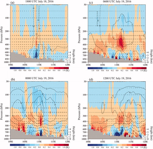
In order to show the analysis differences in the vertical direction between E4CH and E3CH, we show in Fig. 11 four cross sections of the analysis differences of temperature, geopotential height, and wind fields between E4CH and E3CH along a line shown in Fig. 10a at 1800 UTC 18 July, 0000, 0600 and 1200 UTC 19 July 2016. The differences of temperature analysis are seen in all four analysis times near 105°E at 1800 UTC 18 July, where the terrain height is about 3.5 km. The height terrain makes it easy for the assimilation of the AHI CO₂ channel 16 to impact the downstream middle-level atmosphere under the influence of the westerly winds. In fact, the E4CH analyses of temperature in the layer 600–250 hPa are consistently warmer than those of E3CH.

Fig. 11. Cross sections of the analysis differences of temperature (color shading), geopotential height (black contours at interval: 4 m), and wind (black arrow) between E4CH and E3CH (E4CH-E3CH) along the black dashed line in Fig. 10a at 1800 UTC 18 July, 0000, 0600, 1200 UTC 19 July 2016. Grey shaded areas represent the terrain height indicated by the y-axis on the right.

Impacts of the analysis differences among CONV, E3CH and E4CH experiments on the short-range quantitative precipitation forecasts (QPFs) are provided in Figs. 12 and 13. Figure 12 shows the spatial distributions of the 3-h accumulative rainfall observations during 0300–0600 UTC 20 July 2016 (Fig. 12a, case 3), and the 15–18 h model forecasted rainfall amounts CONV, E4CH and E3CH (Fig. 12b-d), valid at the same times as Fig. 12a. The observed precipitation has a cyclone-related comma shape, with the maximum precipitation amount in Beijing and Tianjin, and a narrow band of rainfall affecting many provinces, such as Shandong, Anhui, Henan and Hubei. The second maximum precipitation centre is located north of Henan. All three forecasts captured the comma-shaped precipitation distribution. However, the forecast precipitation patterns from both CONV and E3CH (Fig. 12b, d) are located not as north as the observations (Fig. 12a). The E4CH forecasted precipitation intensity and geographical distribution (Fig. 12c) compares more favourably with observations than both CONV and E3CH, as a result of a deeper cyclone and wetter atmosphere southeast of the cyclone.

Fig. 12. Spatial distributions of (a) the 3-h accumulative rainfall observations during 0300–0600 UTC 20 July 2016, and the 15–18 h model forecasted rainfall amounts by (b) CONV, (c) E4CH and (d) E3CH.

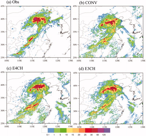
Fig. 13. The equitable threshold scores (ETS) of the 3-h accumulative rainfall at thresholds 10, 15, 20 and 25 mm during from the 24-h model forecasts initialised by the initial conditions of CONV (open cycles), E3CH (stars) and E4CH (solid dots) for case 1 (black), case 2 (red) and case 3 (blue). Grey bars represent the averaged 3-h ETS from CONV (strip), E3CH (twill) and E4CH (solid).

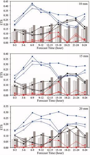
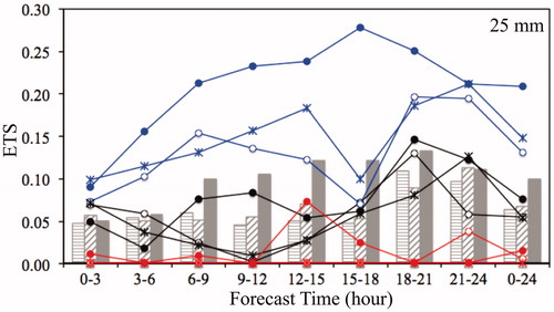
The equitable threat scores (ETSs) (Wilks, 1995) of the 3-h cumulative rainfall at the thresholds 10, 15, 20 and 25 mm for all three cases are provided in Fig. 13. The overall QPF skills are the highest for the large-scale cyclone case 3 (blue curves), second highest for the frontal case 1 (black curves), and the lowest for the small-scale convective case 2 (red curves). The ETSs for all three cases are mostly higher than both CONV and E3CH results, especially at higher thresholds (i.e. 20 and 25 mm) of rainfalls. The ETSs averaged over three cases (grey bars) show that AHI data assimilation of channels 8–10 and 16 produces more significant improvements over the CONV experiment than the assimilation of only channels 8–10 does.

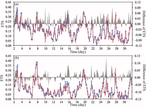
In order to further evaluate the stability of the influence of channel 16 assimilation on precipitation forecast, we also conducted a one-month cycled assimilation and forecast experiment for July 2016. The experimental design is consistent with the three cases. The assimilation starts at 0000 UTC every day, after 1-day of cyclic assimilation, and then makes 24-hour forecast. The ETS results of 3-h precipitation forecast are shown in the Fig. 14. Considering the randomness of heavy rainfall, only comparison results of 3-hour ETS at 1- and 5-mm thresholds are given in the figure, and the verification area is in the middle and lower reaches of the Yangtze River (105–125E, 20–40 N). Red curves represent E3CH, blue curves represent E4CH, and grey shadow represents ETS difference between the two experiments (E4CH-E3CH). It can be seen that in most cases, the score of E4CH is larger than that of E3CH, especially in the second half of July, and the difference is basically positive, which proves that assimilation of channel 16 has a stable improvement effect on precipitation forecast.

Fig. 14. Time series of the 3-h ETS for the E3CH (red) and E4CH (blue) experiments at the (a) 1-, (b) 5-mm thresholds during 2–31 July, 2016. The grey shading represents ETS differences between the two experiments (E4CH-E3CH) on every 3-h.

6. Summary and conclusions

Imager observations of geostationary satellites have high temporal and horizontal resolutions, but a low spectral resolution. The new imagers, such as AHI, have added more water vapour and surface channels, which improves the spectral resolution of geostationary satellite imager observations. Different from other surface-sensitivity channels, the AHI CO₂ channel-16 brightness temperatures are more sensitive to the atmosphere temperature in the lower troposphere than to the surface emissivity. We thus added channel 16 to the AHI data assimilation over land. Numerical data assimilation and forecast results are compared among three experiments: a control experiment without assimilating AHI observations, an experiment assimilating AHI channels 8–10, and an experiment assimilating AHI channels 8–10 and 16. The short-range 24-h QPF skills are significantly further improved by adding AHI channel 16 into AHI data assimilation over land. One-month cycled assimilation experiment also proves that assimilation channel 16 has a stable improvement effect on precipitation forecast.

Adding some other surface-sensitivity channels, such as AHI channels 12 and 14 over bare soil and meadow grass surfaces, including a land-surface data assimilation to obtain an improved surface temperature analysis, assessing added benefits to polar-orbiting environmental satellite observations, selecting clear channels if clouds are confined in low levels, carrying out asymmetric vortex initialisation, and incorporating convective initiation in geostationary satellite data assimilation for numerical weather prediction applications will be our focus of future investigations.

Disclosure statement

No potential conflict of interest was reported by the author.

Additional information

Funding

This research was jointly supported by the National Key R&D Program of China (Grant 2018YFC1507302), and the Nanjing Joint Center of Atmospheric Research Program (Project NJCAR2018ZD01).

References

- Andersson, E., Pailleux, J., Thépaut, J.-N., Eyre, J. R., McNally, A. P. and co-authors. 1994. Use of cloud-cleared radiances in three/four-dimensional variational data assimilation. Q. J. Royal Met. Soc. 120, 627–653. doi:10.1002/qj.49712051707
- Bessho, K., Date, K., Hayashi, M., Ikeda, A., Imai, T. and co-authors. 2016. An introduction to Himawari-8/9—Japan’s new-generation geostationary meteorological satellites. J. Meteorol. Soc. Jpn. 94, 151–183. doi:10.2151/jmsj.2016-009
- Bouttier, F. and Kelly, G. 2001. Observing-system experiments in the ECMWF 4D-Var data assimilation system. Q. J. Royal Met. Soc. 127, 1469–1488. doi:10.1002/qj.49712757419
- Carrier, M. J., Zou, X. and Lapenta, W. M. 2008. Comparing the vertical structures of weighting functions and adjoint sensitivity of radiance and verifying mesocale forecasts using AIRS radiance observations. Mon. Wea. Rev. 136, 1327–1348. doi:10.1175/2007MWR2057.1
- Choi, Y.-S. and Ho, C.-H. 2015. Earth and environmental remote sensing community in South Korea: a review. Remote Sens. Appl. Soc. Environ. 2, 66–76.
- Derber, J. 2003. Enhanced use of radiance data in NCEP data assimilation systems. In: Proceedings of the ITSC XIII, Ste. Adele, Canada.
- Derber, J. C. and Wu, W.-S. 1998. The use of TOVS cloud-cleared radiances in the NCEP SSI analysis system. Mon. Wea. Rev. 126, 2287–2299. doi:10.1175/1520-0493(1998)126<2287:TUOTCC>2.0.CO;2
- English, S. J., Renshaw, R. J., Dibben, P. C., Smith, A. J., Rayer, P. R. and co-authors. 2000. A comparison of the impact of TOVS and ATOVS satellite sounding data on the accuracy of numerical weather forecasts. Q. J. R. Meteorol. Soc. 126, 2911–2932.
- Eyre, J. R. 2007. Progress achieved on assimilation of satellite data in numerical weather prediction over the last 30 years. In: Proceeding of ECMWF Seminar on Recent Developments in of Satellite Observations in Numerical Weather Prediction, ECMWF Publication, Reading UK, 1–27.
- Eyre, J. R., Kelly, G. A., Mcnally, A. P., Andersson, E. and Persson, A. 1993. Assimilation of TOVS radiance information through one dimensional variational analysis. Q. J. Royal Met. Soc. 119, 1427–1463. doi:10.1002/qj.49711951411
- Fertig, E. J., Baek, S.-J., Hunt, B., Ott, E., Szunyogh, I. and co-authors, 2009. Observation bias correction with an ensemble Kalman filter. Tellus 61A, 210–226.
- Garand, L. and Wagneur, N. 2002. Assimilation of GOES imager channels at MSC. In: Proceedings of the ITSC XII, Lorne, Australia.
- Guedj, S., Karbou, F. and Rabier, F. 2011. Land surface temperature estimation to improve the assimilation of SEVIRI radiances over land. J. Geophys. Res. 116, D14107. doi:10.1029/2011JD015776
- Han, Y., Weng, F., Liu, Q. and van Delst, P. 2007. A fast radiative transfer model for SSMIS upper atmosphere sounding channels. J. Geophys. Res. 112, D11121. doi:10.1029/2006JD008208
- Honda, T., Kotsuki, S., Lien, G.-Y., Maejima, Y., Okamoto, K. and co-authors. 2018. Assimilation of Himawari-8 all-sky radiances every 10 minutes: impact on precipitation and flood risk prediction. J. Geophys. Res. Atmos. 123, 965–976. doi:10.1002/2017JD027096
- Honda, T., Miyoshi, T., Lien, G.-Y., Nishizawa, S., Yoshida, R., Adachi, S. A. and co-authors. 2018. Assimilating all-sky Himawari-8 infrared radiances: a case of Typhoon Soudelor (2015). Mon. Wea. Rev. 146, 213–229. doi:10.1175/MWR-D-16-0357.1
- Hong, S.-Y. and Dudhia, J. 2003. Testing of a new non-local boundary layer vertical diffusion scheme in numerical weather prediction applications. In: 20th Conference on Weather Analysis and Forecasting/16th Conference on Numerical Weather Prediction, Seattle, WA.
- Hong, S.-Y. and Lim, J.-O. J. 2006. The WRF singlemoment 6-class microphysics scheme (WSM6). J. Korean Meteor. Soc. 42, 129–151.
- Jones, T. A., Wang, X., Skinner, P., Johnson, A. and Wang, Y. 2018. Assimilation of GOES-13 imager clear-sky water vapor (6.5 mm) radiances into a Warn-on-Forecast system. Mon. Wea. Rev. 146, 1077–1107. doi:10.1175/MWR-D-17-0280.1
- Kazumori, M. 2016. Assimilation of Himawari-8 clear-sky radiance data in JMA’s NWP systems. CAS/JSC WGNE Res. Activ. Atmos. Oceanic Modell. 46, 01.15–01.16.
- Kelly, G. 2008. Preparations and experiments to assimilate satellite image data into high resolution NWP, Tech. Rep. 522, Met Off. Meteorol. Res. and Dev., Exeter, UK.
- Kelly, G. and Thepaut, J.-N. 2007. Evaluation of the impact of the space component of global observing system through observing system experiment, ECMWF publication, Reading UK, 327–346.
- Köpken, C., Kelly, G. and Thépaut, J.-N. 2004. Assimilation of Meteosat radiance data within the 4D-VAR system at ECMWF: assimilation experiments and forecast impact. Q. J. R Meteorol. Soc. 130, 2277–2292. doi:10.1256/qj.02.230
- Köpken, C., Thépaut, J.-N. and Kelly, G. 2003. Assimilation of geostationary WV radiances from GOES and Meteosat at ECMWF. Research report No. 14, EUMETSAT/ECMWF Fellowship programme. ECMWF, Reading, UK.
- Li, X., Zou, X. and Zeng, M. 2019. An alternative bias correction scheme for CrIS data assimilation in a regional model. Mon. Wea. Rev.,147, 809–839.
- Ma, Z., Maddy, E., Zhang, B., Zhu, T. and Boukabara, S. 2017. Impact assessment of Himawari-8 AHI data assimilation in NCEP GDAS/GFS with GSI. J. Atmos. Oceanic Technol. 34, 797–815. doi:10.1175/JTECH-D-16-0136.1
- Minamide, M. and Zhang, F. 2018. Assimilation of all-sky infrared radiances from Himawari-8 and impacts of moisture and hydrometer initialization on convection-permitting tropical cyclone prediction. Mon. Wea. Rev. 146, 3241–3258. doi:10.1175/MWR-D-17-0367.1
- Miyoshi, T., Sato, Y. and Kadowaki, T. 2010. Ensemble Kalman filter and 4D-Var intercomparison with the Japanese operational global analysis and prediction system. Mon. Wea. Rev. 138, 2846–2866. doi:10.1175/2010MWR3209.1
- Montmerle, T., Rabier, F. and Fischer, C. 2007. Relative impact of polar-orbiting and geostationary satellite radiances in the Aladin/France numerical weather prediction system. Q. J. R. Meteorol. Soc. 133, 655–671. doi:10.1002/qj.34
- Qin, Z. and Zou, X. 2018. Direct assimilation of ABI infrared radiances in NWP models. IEEE J. Sel. Top. Appl. Earth Observ. Remote Sens. 11, 2022–2033. doi:10.1109/JSTARS.2018.2803810
- Qin, Z. and Zou, X. 2019. Impact of AMSU-A data assimilation over high terrains on QPFs downstream of the Tibetan Plateau. J. Meteorol. Soc. Jpn. 97, 1137–1154. doi:10.2151/jmsj.2019-064
- Qin, Z., Zou, X. and Weng, F. 2013. Evaluating added benefits of assimilating GOES imager radiance data in GSI for coastal QPFs. Mon. Wea. Rev. 141, 75–92. doi:10.1175/MWR-D-12-00079.1
- Qin, Z., Zou, X. and Weng, F. 2017. Impacts of assimilating all or GOES-like AHI infrared channels radiances on QPFs over Eastern China. Tellus A Dynam. Meteorol. Oceanogr. 69, 1345265. doi:10.1080/16000870.2017.1345265
- Schmit, T. J., Griffith, P., Gunshor, M. M., Daniels, J. M., Goodman, S. J. and co-authors. 2017. A closer look at the ABI on the GOES-R series. Bull. Am. Meteor. Soc. 98, 681–698. doi:10.1175/BAMS-D-15-00230.1
- Shao, H., Derber, J., Huang, X.-Y., Hu, M., Newman, K. and co-authors. 2016. Bridging research to operations transitions: status and plans of community GSI. Bull. Amer. Meteor. Soc. 97, 1427–1440. doi:10.1175/BAMS-D-13-00245.1
- Shen, Y., Zhao, P., Pan, Y. and Yu, J. 2014. A high spatiotemporal gaugesatellite merged precipitation analysis over China. J. Geophys. Res. Atmos. 119, 3063–3075. doi:10.1002/2013JD020686
- Stengel, M., Lindskog, M., Undén, P. and Gustafsson, N. 2013. The impact of cloud-affected IR radiances on forecast accuracy of a limited-area NWP model. Q. J. R. Meteorol. Soc. 139, 2081–2096. doi:10.1002/qj.2102
- Stengel, M., Lindskog, M., Undén, P., Gustafsson, N. and Bennartz, R. 2010. An extended observation operator in HIRLAM 4D-VAR for the assimilation of cloud-affected satellite radiances. Q. J. R. Meteorol. Soc. 136, 1064–1074. doi:10.1002/qj.621
- Stengel, M., Undén, P., Lindskog, M., Dahlgren, P., Gustafsson, N. and co-authors. 2009. Assimilation of SEVIRI infrared radiances with HIRLAM 4D-Var. Q. J. R. Meteorol. Soc. 135, 2100–2109. doi:10.1002/qj.501
- Schmetz, J., Pili, J., Tjemkes, S., Just, D., Kerkmann, J. and co-authors. 2002. An introduction to Meteosat Second Generation (MSG). Bull. Am. Meteorol. Soc. 83, 977–992. doi:10.1175/BAMS-83-7-Schmetz-2
- Szyndel, M., Kelly, G. and Thépaut, J.-N. 2005. Evaluation of potential benefit of assimilation of SEVIRI water vapor radiances data from Meteosat-8 into global numerical weather prediction analyses. Atmos. Sci. Lett. 6, 105–111. doi:10.1002/asl.98
- Wang, Y., Liu, Z., Yang, S., Min, J., Chen, L. and co-authors. 2018. Added value of assimilating Himawari-8 AHI water vapor radiances on analyses and forecasts for "7.19" severe storm over north China. J. Geophys. Res. 123, 3374–3394. doi:10.1002/2017JD027697
- Wilks, D. S. 1995. Statistical Methods in the Atmospheric Sciences: An Introduction. Academic, San Francisco, CA, p. 467.
- Wu, W.-S.,Purser, R. J. andAndparrish, D. F. 2002. Three-dimensional variational analysis with spatially inhomogeneous covariances. Mon. Wea. Rev 130, 2905–2916.
- Yang, J., Zhang, Z., Wei, C., Lu, F. and Guo, Q. 2017. Introducing the new generation of Chinese geostationary weather satellites, Fengyun-4. Bull. Am. Meteor. Soc. 98, 1637–1658. doi:10.1175/BAMS-D-16-0065.1
- Zhang, F., Minamide, M. and Clothiaux, E. E. 2016. Potential impacts of assimilating all-sky infrared satellite radiance from GOES-R on convection-permitting analysis and prediction of tropical cyclones. Geophys. Res. Lett. 43, 2954–2963. doi:10.1002/2016GL068468
- Zhang, Y., Zhang, F. and Stensrud, D. 2018. Assimilating all-sky infrared radiancefrom GOES-16 ABI using an ensemble Kalman filter for convection-allowing severe thunderstorms prediction. Mon. Wea. Rev. 146, 3363–3381. doi:10.1175/MWR-D-18-0062.1
- Zheng, W., Wei, H., Meng, J., Ek, M., Mitchell, K. and co-authors. 2009. Improvement of land surface skin temperature in NCEP operational, paper presented at 23rd Conference on Weather Analysis and Forecasting/19th Conference on Numerical Weather Prediction, Am. Meteorol. Soc., Omaha, NE.
- Zhu, Y.,Derber, J.,Collard, A.,Dee, D.,Treadon, R. and co-authors. 2014. Enhanced radiance bias correction in the National Centers for Environmental Prediction's Gridpoint Statistical Interpolation data assimilation system. QJR. Meteorol. Soc. 140, 1479–1492. doi:10.1002/qj.2233
- Zhuge, X. and Zou, X. 2016. Test of a modified infrared only ABI cloud mask algorithm for AHI radiance observations. J. App. Meteor. Climatol. 55, 2529–2546. doi:10.1175/JAMC-D-16-0254.1
- Zou, X., Qin, Z. and Weng, F. 2011. Improved coastal precipitation forecasts with direct assimilation of GOES 11/12 imager radiances. Mon. Wea. Rev. 139, 3711–3729. doi:10.1175/MWR-D-10-05040.1
- Zou, X., Qin, Z. and Zheng, Y. 2015. Improved tropical storm forecasts with GOES-13/15 imager radiance assimilation and asymmetric vortex initialization in HWRF. Mon. Wea. Rev. 143, 2485–2505. doi:10.1175/MWR-D-14-00223.1
- Zou, X., Weng, F., Zhang, B., Lin, L., Qin, Z. and Tallapragada, V. 2013. Impacts of assimilation of ATMS data in HWRF on track and intensity forecasts of 2012 four landfall hurricanes. J. Geophys. Res. Atmos., 118, 11558–11576. doi:10.1002/2013JD020405
- Zou, X., Zhuge, X. and Weng, F. 2016. Characterization of bias of advanced Himawari Imager observations from NWP background simulations using CRTM and RTTOV. J. Atmos. Oceanic Technol. 33, 2553–2567. doi:10.1175/JTECH-D-16-0105.1