Designing and evaluating regional climate simulations for high latitude land use land cover change studies

Abstract

High latitude regions are undergoing substantial land use and land cover change (LULCC) arising partly from a changing climate (e.g. greening of the Arctic) and climate mitigation policies (e.g. afforestation). Despite these ongoing changes, the impacts of LULCC in high latitudes are poorly understood. Studies to reduce this knowledge deficit primarily deploy regional climate models (RCMs) as observations of key variables for LULCC studies are scarce in high latitude regions. As such it is important to understand the limitations of RCMs and identify best practices for designing regional climate modelling experiments for LULCC studies at high latitudes. In this study, twelve 10-year simulations are performed over the Scandinavian Peninsula; six at convection permitting scales (dx ∼ 3 km) and six at non-convection permitting scales (dx ∼ 15 km). Two of the convection permitting simulations model the present and future climate conditions over the Scandinavian Peninsula. The present-day simulation is comprehensively evaluated for multiple variables (e.g. surface air temperature at 2 m, precipitation) using multiple sources of observations (stations, reanalysis & blended satellite products) where available. Results from the model evaluation points to the need for further model improvement in simulating precipitation and related snow processes as well as the need for observations of surface energy fluxes at high latitudes for evaluation. The remaining eight simulations differ in terms of grid spacing, background climate state (present or future climate), and land cover (conversion of grasslands to evergreen needleleaf or mixed forest). Our study highlights the strengths and limitations of common RCM design considerations, such as simulation length (single year vs. multi-years), background climate state (present vs. future climate) and model resolution (convection permitting vs. non-convection permitting). A key recommendation is that high-latitude modeling studies of LULCC should prioritize computational resources for multi-decadal and ensemble simulations over short, single experiment simulations at convection permitting scales.

Keywords:

• land use change
• land cover change
• land-atmosphere interactions
• WRF model
• convection permitting
• high-latitudes

1. Introduction

It is now widely accepted that land use and land cover change (LULCC) exert substantial impact on the climate system (Pielke et al., 2011; Mahmood et al., 2014). This impact occurs through biogeophysical and biogeochemical processes. Specifically, LULCC can impact regional atmospheric circulation, moisture budgets, surface fluxes, precipitation and temperatures (Mahmood et al., 2014). Such studies emphasize that the effects of LULCC, especially at high latitudes, are poorly understood as most research has focused on the tropical and temperate zone. There is growing interest in LULCC impacts in high latitude ecosystems under current projections of climate change. Some of these include the latitudinal and altitudinal expansion of treeline, the natural succession of historically open landscapes (Bartsch et al., 2016), and afforestation as a climate mitigation action (Bastin et al., 2019).

LULCC affects climate at various scales, ranging from local to regional to sub-continental and global scales. While globally, biogeochemical effects from LULCC are considered larger than biogeophysical effects (Findell et al., 2007), regionally, biogeophysical effects play a more important role (de Noblet-Ducoudré et al., 2012). Recent studies emphasize that biogeophysical effects are primarily responsible for the LULCC impact on the regional climate at high latitudes where snow cover controls albedo (Davin et al., 2020).

There are some observational studies on the impact of LULCC on the regional climate at high latitudes, e.g. those obtained with flux towers (Lee et al., 2011) or remote sensing data (Bright et al., 2017). Such observation-based studies often rely on space-for-time substitution (e.g. open landscape compared to different stages of forest growth nearby). Unfortunately, it is often difficult to isolate LULCC signals in observational data mixed among with climatic factors, particularly when the climatic conditions across the comparisons are not identical (Chen and Dirmeyer, 2020). In addition, observational methods cannot provide quantitative assessments of the feedbacks and processes associated with LULCC and the climate. Therefore, regional climate modeling (RCM) studies are crucial to understanding the effects of LULCC on the climate system.

However, there are emerging issues in the design of regional climate modelling experiments to understand LULCC at high latitudes, e.g. model resolution. Regional climate modelling studies at the so-called ‘convection permitting’ scales (i.e. dx < 4 km) are becoming more widespread. However, they are very expensive computationally and this necessitates certain assumptions in the design of regional modelling experiments of LULCC and climate. For example, some studies assume that a simulation duration of 1-year (Qu et al., 2013; Cao et al., 2015; Laux et al., 2017; Wagner et al., 2017) or grid spacing of 50 km is sufficient to ascertain the LULCC impact, while others assume that assessing LULCC impacts under current climate conditions will also apply under future climate conditions (e.g. Georgescu et al., 2009; Wang et al., 2018; Hu et al., 2019; Davin et al. 2020). While there are clear benefits of going to these very high resolutions for studying precipitation and extreme events, no previous study has identified the benefits of these scales for LULCC studies at high latitudes. This raises the important question of whether or not convection-permitting scales are necessary for modelling studies on LULCC and climate at high latitudes where surface albedo is the key factor in land-atmosphere interactions.

In this study, we explore the best practices in regional climate modelling for studying the impacts of high latitude LULCC on the regional climate. We focus on addressing 1) limitations for evaluating RCM simulations at high latitudes, 2) the relevance of convection permitting scales in high latitude LULCC studies, and 3) the importance of simulation length. We choose surface temperature as the key variable since previous studies (e.g. Breil et al., 2020) have demonstrated that this variable exhibits the clearest LULCC. Precipitation and climate extremes were also investigated, but no statistically significant LULCC impact was found and as such the results are not shown here.

2. Methods

2.1. Model configuration

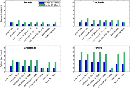
The European Centre for Medium Range Weather Forecasting Interim Reanalysis (ERA-Interim) is downscaled over the period 1996–2005 with the Advanced Research Weather Research and Forecasting (WRF) model version 3.9.1.1 (Skamarock et al., 2008). The WRF model has been widely used in regional climate modeling studies (e.g. Mooney et al., 2013, 2016; Katragkou et al., 2015; Bruyere et al., 2017). The domains used in this study are shown in Fig. 1. The outer domain has 347 × 266 (east-west x north-south) grid points and uses a grid spacing of 15 km, while the inner domain has 466 × 601 grid points and a grid spacing of 3 km. The model has 51 vertical levels and a model top of 50 hPa. This study uses the sigma coordinate system described in Skamarock et al. (2008). Based on the Mooney et al. (2013) assessment of WRF physical parameterizations for regional climates over Europe, the following physical parameterizations were used in the WRF model: the Thompson microphysics (Thompson et al., 2008), RRTMG longwave and shortwave radiation schemes (Iacono et al., 2008), Yonsei University planetary boundary layer scheme (Hong et al., 2006), the revised Monin-Obukhov surface layer scheme (Jimenez et al., 2012), the Kain-Fritsch cumulus scheme (Kain, 2004; on the 15 km domain only), and the Noah Multi-Physics (Noah-MP; Niu et al., 2011) land surface model. In order to properly initialize the Noah-MP land surface model (LSM), it is run repeatedly for the year 1995 until soil-state variables reach their equilibrium state. Following Chen et al. (2016), equilibrium is reached when the difference between the annual mean of two consecutive years is less than 0.1%. The number of years required for the soil to reach this equilibrium state is often referred to as the ‘spin-up’ period. Figure 2 shows the length of the model spinup period for both the 15 km and 3 km domains for important land-atmosphere variables such as soil temperature, soil moisture, latent heat fluxes and sensible heat fluxes. The analysis averages the values for each variable for all grid boxes in different land use categories, e.g. grasslands or tundra. Forests and croplands have the shortest spin-up periods of 2 to 3 years and there is very little difference in the spin-up period between the different resolutions. However, grasslands require a longer spin-up period of 2–5 years depending on the variable for the domain with a 15 km grid spacing while the 3 km domain needs between 2–6 years depending on the variable of interest. Tundra regions require a substantially longer time to spin-up compared to the other land use categories with spin-up times usually needing 4–6 years for the 15 km domain and typically 9–10 years for the 3 km domain. Based on this analysis, a spin-up period of 10 years is used in this study for all simulations.

Fig. 1. (a) Domains used in the WRF simulations. The outer domain is simulated at a grid spacing of 15 km while the inner domain is simulated at 3 km. (b) Enlarged image of the 3-km domain shown in (a) and marked here in red. (c) the USGS land cover for the 15-km domain over the area of interest - Scandinavian Peninsula. (d) Same as (c) except for the 3 km domain. (e) Grid boxes with land cover changed to either evergreen needleleaf (Afforestation simulation) or mixed forest (Natural Succession). (f) Same as (e) except for the 3 km domain.

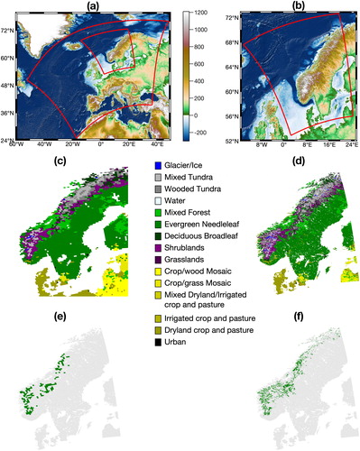
Fig. 2. Number of years required for surface spinup over (a) forested areas, (b) croplands, (c) grasslands, and (d) tundra regions.

2.2. Experiment design

Limited by the computational demand for a large domain (52^oN to 72^oN and 3^oE to 22^oE) at very high resolution for a 10-year period, twelve simulations were performed to explore the possible impacts of current afforestation policies under consideration in Norway on the local and regional climate (Haugland et al., 2013). The twelve simulations consist of three different land use land cover changes, two different climate scenarios, and two different resolutions. The current policy considers the conversion of existing open spaces to forested regions by active afforestation with evergreen needleleaf trees. Alternatively, abandonment of historically open landscapes due to urbanization leads to natural succession dominated by mixed broadleaf deciduous and needleleaf evergreen trees.

Six simulations which differ by grid spacing and land cover are performed under historical climate conditions and six similar simulations are performed under a future climate scenario which is designed to represent the climate in the middle of the century under the 8.5 Representative Concentration Pathway RCP8.5; this is described in more detail in the next section. The first set of simulations (hereafter called Control-historical or Control-RCP8.5 depending on the background climate) uses present day land cover as described by the United States Geological Survey (Fig. 1c,d). This simulation serves two purposes. Firstly, it provides the basis for our evaluation of the model’s ability to simulate the regional climate and secondly, it serves as the reference climate for the two quasi-idealized land cover scenarios. In the quasi-idealized simulations, the land cover currently identified as grasslands and shrublands in the USGS land cover data (Fig. 1e,f) were replaced with forests; this amounted to a total of 3998 grid boxes changing to forests in the 3 km simulations and 156 in the 15 km simulations. Grasslands and Shrublands above timberline (approximated to 1,100 m based on Odland (2015)) were excluded from the conversion. The two quasi-idealized simulations differ by the type of forest. One simulation uses evergreen needleleaf to represent active afforestation (hereafter called Afforest-historical or Afforest-RCP8.5 depending on the background climate) and the other simulation uses mixed forest to represent the natural succession of open spaces to forests (hereafter called Natural-historical or Natural-RCP8.5 depending on the background climate). The results for the Afforest- and Natural- simulations are almost identical. As such only the Afforest-historical and Afforest-RCP8.5 results are presented in the main manuscript with corresponding figures for Natural-historical and Natural-RCP8.5 presented in the Supplementary Material (Figures S1–S3). The analysis of two types of simulations which differ only by surface properties (e.g. surface roughness and albedo) increases the robustness of our findings.

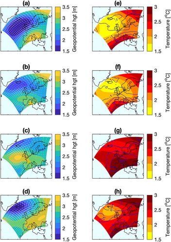
Fig. 3. Pseudo-Global Warming delta for the 700 hPa geopotential height (colours) and the 700 hPa winds (arrows) in Winter (a), Spring (b), Summer (c) and Autumn (d). Pseudo Global Warming delta for temperature (colours) and relative humidity (contours) at 700 hPa for Winter (e) and Spring (f), Summer (g) and Autumn (h).

2.3. Pseudo global warming (PGW) method

A pseudo-global warming technique similar to the approach applied in Liu et al. (2017) and Parker et al. (2018) is used to create a future climate simulation. The 10-year future simulation was forced with 6 hourly ERA-Interim data that was perturbed by the addition of a monthly change in the climate between a future 30-year period (2035–2065) and a reference 30-year period (1975–2005). The future period uses RCP8.5 centred on the middle of this century which corresponds to approximately 1.5 °C warming globally. The perturbed future climate was calculated using the following formula: $$X_{\mathit{PGW}\left(6h\mathit{rly}\right)}=X_{\mathit{ERAI}\left(6h\mathit{rly}\right)}+\Delta {\overline{X}}_{\mathit{GCM}\mathit{,}mon}$$ where X represents one of the following perturbed variables: horizontal winds, temperature, geopotential, specific humidity, sea surface temperature, soil temperature, sea level pressure and sea ice.

$\Delta {\overline{X}}_{\mathit{GCM},\mathit{mon}}$ is calculated for each month by: $$\Delta {\overline{X}}_{\mathit{GCM}\mathit{,}mon}={\overline{X}}_{2036-2065,mon}-{\overline{X}}_{1976-2005,mon}$$ where ${\overline{X}}_{ ,mon}$ represents the monthly mean of the variable X over the entire 30-year period derived from the ensemble mean of the CMIP5 models listed in Table 1.

Table 1. CMIP5 GCMs used for deriving the climate perturbations for the PGW simulations.

Model name	Grid resolution (lats × lon) [degrees]	No. vert. levels	No. ensemble members from historical simulation	No. ensemble members from RCP8.5 simulation	Ensemble members used	Names of member realisations
ACCESS1-3	1.25 × 1.875	17	3	1	1	r1i1p1
CanESM2	2.79 × 2.81	22	5	5	3	r1i1p1, r2i1p1, r3i1p1
CCSM4	0.94 × 1.25	17	6	6	3	r1i1p1, r2i1p1, r6i1p1
CESM1-CAM5	0.94 × 1.25	17	3	3	3	r1i1p1, r2i1p1, r3i1p1
CMCC-CM	0.75 × 0.75	17	1	1	1	r1i1p1
CNRM-CM5	1.40 × 1.41	17	10	5	3	r2i1p1, r4i1p1, r6i1p1
CSIRO-Mk3-6-0	1.87 × 1.88	18	10	10	3	r1i1p1, r2i1p1, r3i1p1
GFDL-CM3	2.00 × 2.50	23	5	1	1	r1i1p1
GFDL-ESM2M	1.52 × 2.50	17	1	1	1	r1i1p1
GISS-E2-H	2.00 × 2.50	17	5	2	2	r1i1p1, r2i1p1
HadGEM2-CC	1.2 × 1.875	23	3	3	3	r1i1p1, r2i1p1, r3i1p1
HadGEM2-ES	1.25 × 1.875	17	4	4	1	r3i1p1
INM-CM4	1.50 × 2.00	17	1	1	1	r1i1p1
IPSL-CM5A-MR	1.27 × 2.50	17	3	1	1	r1i1p1
MIROC5	1.40 × 1.41	17	4	3	3	r1i1p1, r2i1p1, r3i1p1
MIROC-ESM	2.79 × 2.81	35	3	1	1	r1i1p1
MPI-ESM-LR	1.87 × 1.88	25	3	3	3	r1i1p1, r2i1p1, r3i1p1
MPI-ESM-MR	1.87 × 1.88	25	3	1	1	r1i1p1
MRI-CGCM3	1.12 × 1.12	23	4	1	1	r1i1p1

Figure 3 shows the perturbed climate from the GCM ensemble mean for the geopotential height, winds, and temperature at 700 hPa for each season. The weak changes in wind (<1 m/s) and geopotential (<4 m) indicate that the large-scale circulation remains largely unchanged between 1976–2005 and 2036–2065 for the ensemble mean in this region. Slightly larger perturbations to the 700 hPa winds occur in Winter and Spring. Temperature at 700 hPa is substantially perturbed (1.5–3.5 °C) in all seasons with the largest increases in Summer and Autumn (∼2.0–3.5 °C) compared to Winter and Spring (∼1.5–2.5 °C). Perturbations to the relative humidity at 700 hPa are between −4% and 2%. Similar results are obtained for the winds, geopotential, temperature and relative humidity at the 250 hPa and 850 hPa levels (not shown). Overall, these results show that the future climate perturbation consists primarily of robust temperature and moisture enhancements with only weak changes to the circulation pattern.

2.4. Gridded datasets

The following gridded datasets were used to evaluate model performance against observational data. The climate variables used in model evaluation include surface air temperature at 2 m (T2m), precipitation, snow cover, and snow depth, where available.

2.4.1. Reanalysis data

The European Centre for Medium Range Weather Forecasting’s (ECMWF) interim (ERA-Interim) Re-analysis is used to force the WRF model at the boundaries and for providing initial conditions to WRF. This data was obtained from the ECMWF data server (https://apps.ecmwf.int/datasets/data/interim-full-daily). ERA-Interim data used by the WRF model was obtained on a fixed grid of 0.75° on all available pressure levels along with the necessary surface level data described in the WRF model.

2.4.2. SeNorge

The seNorge2018 version 18.12 high-resolution gridded dataset used in this study was produced by the Norwegian Meteorological Institute (MET Norway) and obtained from http://thredds.met.no/thredds/catalog/senorge/catalog.html. The seNorge daily estimates of precipitation and temperature has a grid spacing of 1 km that covers the period from 1957 to the present day. Further details of the seNorge precipitation product and its methodology are provided in Lussana et al. (2018a, 2018b) while details of the seNorge temperature products can be found in Lussana et al. (2019). A known limitation of the precipitation dataset is the underestimation of precipitation in the high mountainous regions of southern Norway (Lussana et al. 2018a) resulting from the low station density in that region. Lussana et al. (2018a, 2018b) demonstrate that the precision of the estimates for daily temperature varies between 0.8 and 2.4 °C with winter minimum temperature having a bias between 2 °C and 3 °C in data sparse regions (Lussana et al., 2019).

2.4.3. Station data

Station data are obtained from the Norwegian meteorological service, MET Norway. Data is quality checked using ‘buddy checks’, removing unrealistic extremes, and unrealistically long periods with zero precipitation. The analysis includes only those stations where there is less than 10% missing data over the period 1996–2005. Unlike the temperature and snow depth data, the precipitation data is daily accumulated from 0600 UTC to 0600 UTC and the modelled data is processed to match this accumulation period.

2.4.4. Globsnow2 monthly fractional snow cover

The European Space Agency Data User Element GlobSnow2 Snow Extent data used in this study is a satellite based (level 3B) gridded observational product of monthly fractional snow cover derived from the visual-to-thermal part of the electromagnetic spectrum. Since the data are derived from optical sensors, there are no data available for the dark winter months of December and January at these latitudes. The GlobSnow2 Monthly Fractional Snow Cover product covers the northern hemisphere on a 0.01° (∼1 km) grid over the period 1995–2012. GlobSnow2 data used in this study was obtained from http://www.globsnow.info. Further details of this data, including the algorithms and sensors used to produce this data, are provided in Metsämäki et al. (2015).

2.4.5. E-OBS gridded dataset

The E-OBS gridded dataset is an observation based gridded data product over Europe at daily intervals. The version of the data used in this study was v20.0e. The data was obtained on a regular 0.1° (∼10–12 km) grid from https://surfobs.climate.copernicus.eu/dataaccess/access_eobs.php. Further details of the E-OBS gridded dataset and its limitations can be found in Cornes et al. (2018).

3. Results

3.1. Model evaluation

This section presents the results of the evaluation of the WRF model’s ability to simulate the regional climate of Norway during the period 1996–2005 with a focus on key variables for LULCC studies such as temperature and snow. An evaluation of other important variables such as surface energy fluxes and soil temperature are hampered by the lack of observations in this region.

3.1.1. 2m-Air temperature

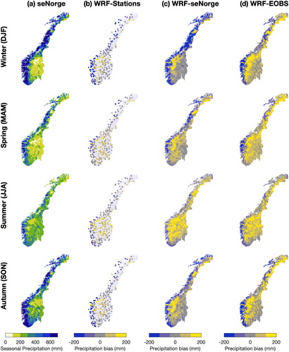
Figure 4 shows the seasonal 2 m-air temperature (T2m) over the 10-year period 1996–2005 from the SeNorge gridded observational product along with the seasonal biases for the Control simulation calculated using three different observational products: station observations, seNorge gridded observations (1 km), and E-OBS gridded observations (∼10–12 km). As Fig. 4 shows, T2m over Norway has a distinct seasonal cycle that varies spatially. The mean summer values for T2m during 1996–2005 range between 10–20 °C in low lying regions with lower values in high mountainous regions. Winter T2m values during this period are much colder and range from −4.8 °C in regions below 800 m to −8.7 °C in regions above 800 m.

Fig. 4. (a) Seasonal surface air temperature at 2 m (T2m) from the gridded observational product seNorge2018. (b) Bias in seasonal simulated T2m based on observed station data. (c) Bias in seasonal simulated T2m based on seNorge2018 gridded observational product. (d) Bias in seasonal simulated T2m based on EOBS gridded observational product.

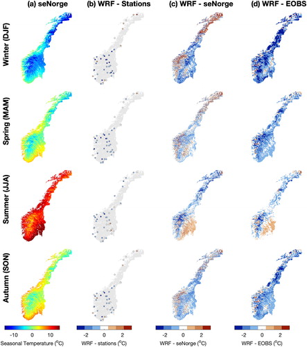
There are strong seasonal variations in the bias. T2m biases in WRF are lowest in spring and autumn with values typically between −1 °C and +1 °C. The strongest biases are in winter and summer, and vary between −2 °C and +2 °C. There are also spatial variations in the temperature biases of winter and summer. In winter, the coldest biases are in the east where they average approximately −0.8 °C and the warmest biases are in the north with an average of approximately 1.0 °C. In summer the coldest biases are to the west (∼−0.6 °C) and the warmest are to the east (∼0.5 °C). These biases lie within the range of precision for the seNorge estimates (Lussana et al., 2019). The model biases when compared to the station data (Fig. 4b) are similar to those obtained in comparison to seNorge. However, the model biases are stronger when compared to E-OBS gridded data. This may be a result of the coarser grid spacing of E-OBS (∼10–12 km).

3.1.2. Precipitation

Figure 5 shows the seasonal precipitation in Norway over the 1996–2005 period based on the seNorge high resolution gridded product. Precipitation in Norway exhibits a strong spatial pattern that is partially due to its long coastline and complex topography. Previous studies (e.g. Barstad and Caroletti, 2013; Sandvik et al., 2018) have highlighted deficiencies in WRF simulations such as the deposition of precipitation of propagating frontal systems too far inland. This leads to an underestimation of observed precipitation along the western coastline and an overestimation of precipitation slightly further inland. Both of these biases are present in our Control simulation (Fig. 5) when compared to both the station observations and the gridded observation products of seNorge and E-OBS. The overestimation of precipitation shown in Fig. 4 does not result exclusively from the aforementioned deficiency in WRF. It is important to recognize that this bias is likely exaggerated by the limitations of the gridded observational product. In this remote region of western Norway where the climate is characterized by high, steep terrain, there are only a few stations and these also suffer from undercatch. This leads to an underestimation of precipitation in the gridded observations (Lussana et al., 2018a, 2018b). As such, biases in this region are likely due to deficiencies in both the observed and the simulated product. The eastern part of southern Norway has the lowest bias in all seasons except summer when precipitation is mostly convective; this is also the season when eastern Norway receives most of its precipitation. These biases in our simulated precipitation are consistent with previous studies on the simulation of precipitation over Norway (Mayer et al., 2015; Pontoppidan et al., 2017; Sandvik et al., 2018). It is beyond the scope of this study, however, to solve this challenge. Regardless of these biases in our WRF simulations, analysis of the impacts of land use changes on temperature is largely unaffected by them.

Fig. 5. Same as Fig. 4 except for precipitation.

3.1.3. Snow cover and depth

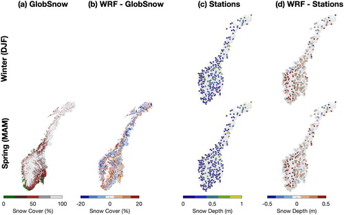
Fractional snow cover over Norway from the GlobSnow satellite product for spring is shown in Fig. 6 along with the bias in the modelled fractional snow cover. Simulated snow cover is reasonably well represented in the model. Model biases range from −20% to +20% which is within the range of one standard deviation of the GlobSnow product. Figure 6 also shows a comparison of the modelled winter and spring snow depth with observations from stations. There are large biases in the modelled snow depths at almost all snow stations. These biases are outside the range of observational uncertainty and likely arise from the over estimation of precipitation by the WRF model shown in Fig. 5.

Fig. 6. (a) Spring fractional snow cover from GlobSnow2. (b) Model bias in the spring fractional snow cover simulated by WRF over the 3 km domain. (c) Winter and spring snow depth at stations. (d) Model bias in snow depth for winter and spring simulated by WRF over the 3 km domain.

3.2. Role of grid spacing, simulation length and background climate in the simulated temperature response

3.2.1. Impact of model resolution

Figure 7 shows the daytime and night-time surface (or skin) temperature response to the aforementioned LULCC in both the 15 km and 3 km domains; only grid boxes that exhibit a statistically significant change at the 95% level are shown. Even in the complex terrains of Norway, the overall patterns were similar in evergreen and mixed forest scenarios (Fig. S1). There is a clear seasonal signal in the surface temperature response to the LULCC. In winter and spring, converting the open spaces to forestry warms the surface, while in Summer the surface cools. Autumn shows no statistically significant response to the LULCC. Qualitatively, Fig. 7 also shows that there is very little difference between the temperature response in the 15 km and 3 km domains. A more quantitative analysis of these differences is presented in Fig. 8.

Fig. 7. Simulated daytime (12 UTC) surface temperature response to converting the land cover from grasslands to evergreen in the 15 km simulation (top row) and in the 3 km simulation (2nd row) for each of the four northern hemisphere seasons (columns) over the historical period (1996–2005). Only grid boxes that exhibit a statistically significant change at the 95% level are shown.

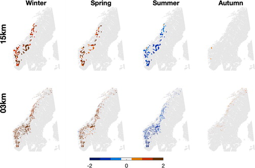
Fig. 8. (a) Spatial mean and variability of the daytime surface temperature response for each season for both the 15 km (red) and 3 km (blue) simulations. (b) Percentage of LULCC grid boxes that show a statistically significant (95% confidence level) surface temperature response to the LULCC during the daytime. (c) and (d) same as (a) and (b) except for night-time.

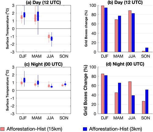
The spatial mean and spatial variation of the daytime surface temperature response for both grid spacings is shown in Fig. 8a for the Afforest-historical simulations while the Natural-historical plots are shown in Fig. S2a. For all forestry types, the 3 km simulations have slightly larger spatial variability and slightly stronger response to the LULCC in all three seasons. Figure 8b shows the percentage of LULCC grid boxes that exhibit a statistically significant temperature response during the day. The percentage varies from season-to-season, but it is not influenced by grid spacing. Figure 8c shows the spatial mean and variability of the surface temperature response at night. There is a weak seasonal signal in the surface temperature response to the LULCC at night. There is very little difference in the mean surface temperature response between the different grid spacings. However, Fig. 8d shows that there are differences in the percentage of LULCC grid boxes whose surface temperature experiences a statistically significant response to the LULCC. In spring and autumn, a greater percentage of grid boxes in the 3 km simulations respond to the LULCC while in winter the 15 km simulations show a greater percentage of grid boxes responding to LULCC.

3.2.2. Impact of length of simulation

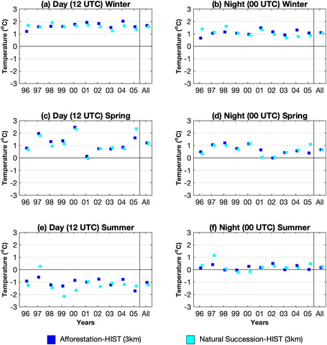
Figure 9 shows the daytime and night-time seasonal surface temperature response to the LULCC for each year of the 15 km and 3 km simulations under the historical climate. All LULCC grid boxes are included in the analysis. Also included is the corresponding values for the entire 10-year period which is labelled as ‘All’ in the x-axis. Year-to-year variability is low in both the daytime and night-time winter values. However, the year-to-year values change considerably in the daytime spring values ranging from approximately 0 °C to 2.7 °C. There is also variability in the night-time spring temperature with values ranging from 0 °C to 1.2 °C for the 3 km simulations. Daytime temperature responses also show a considerable variability from year to year with 1997 showing a value for Natural-Succession experiments of 0.3 °C while most show approximately −1 °C and 1999 showing a temperature response lower than −2 °C. With the exception of daytime winter values, there is considerable variability in the surface temperature response from year-to-year. Another noteworthy observation is that the LULCC temperature response for the Afforestation-Historical simulations sometimes differ by 1 °C or more. This is particularly evident in 1999 where the daytime results suggest that the surface temperature response depends on forest type which contradicts the results in most of the other years.

Fig. 9. (a) Mean daytime surface temperature response to LUC for winter of each year (96 - 05) and for the entire 10-year period (marked ‘All’ on x-axis). (b) same as (a) except for night-time. (c) and (d) Same as (a) and (b) except for spring. (e) and (f) Same as (a) and (b) except for summer.

3.2.3. Impact of background climate state

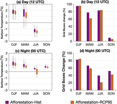
Figure 10 summarizes the surface temperature response to the conversion of grasslands to forest under different background climate states. For this study ‘background climate’ is defined as either ‘historical’ or ‘future’ from CMIP5 (see methods) with their attendant external forcings: greenhouse gas concentrations, aerosols, orbital forcing, etc. Figure 10a shows the spatial mean and variability of the daytime surface temperature response for both types of forestry in the 3 km simulations for the historical and future climates. Simulations of the daytime surface temperature response to the LULCC are only slightly influenced by the background climate. In other words, for the same LULCC, changing the external climate forcing (i.e. historical or future) has minimal effect. In winter and spring the surface temperature response is slightly lower in the future climate simulation compared to the historical climate simulation. This can be understood by the reduced snow cover in the future climate. This effect is also noticed in the percentage of grid boxes that exhibit a statistically significant temperature response (Fig. 10b). In spring, more grid boxes in the historical climate experience a temperature response than in the future climate; this may be a result of earlier snowmelt in the future climate. Night time surface temperatures show a similar pattern (Fig. 10c,d).

Fig. 10. (a) Spatial mean and variability of the daytime surface temperature response from the 3 km simulations for each season for different background climates: historical climate (purple) and Mid-Century RCP8.5 climate (brown). (b) Percentage of LULCC grid boxes that show a statistically significant surface temperature response (95% confidence level) to the LULCC during the day. (c) and (d) same as (a) and (b) except for night-time.

4. Discussion and conclusions

An evaluation framework has been presented for evaluating the performance of regional climate simulations for studies on land-atmosphere interactions over the Scandinavian peninsula. Evaluations of RCMs typically include comparisons of variables such as T2m, precipitation, sea level pressure, upper atmosphere winds and temperature (e.g. at the 850 hPa and 500 hPa level). In RCM applications specifically designed for studies of land-atmosphere interactions, this should be extended to include relevant variables such as surface energy fluxes, soil moisture and soil temperature in low- and mid-latitude regions. In high latitude regions such as Norway, they should also include evaluations of snow as surface albedo is the key driver of the climate response to LULCC at high latitudes. Furthermore, model evaluations should compare the model simulation to multiple sources of observations as outlined in Prein and Gobiet (2017). Despite the clear importance of this type of model evaluation, it is hampered by a lack of high quality, long term observational data of the surface energy budget, soil moisture, soil temperature, and snow cover and depth in many high latitude regions, including Norway.

At high latitudes, the climate response to LULCC is primarily driven by changes in radiative fluxes at the surface due to changes in surface albedo during the snow seasons; this contrasts with lower latitudes where the climate response is driven by changes in the surface sensible and latent heating. We find that simulations of a decade or longer are required to determine a robust temperature response to LULCC, increasing model resolution from 15 km to 3 km only marginally changes the results, and background climate (present day vs. future) may influence the temperature response to LULCC. This gives us an opportunity to make recommendations for future studies.

Analysis of the year-to-year temperature response to LULCC showed considerable variability in spring and summer temperatures. These results suggest that single year experiments are dependent on the year chosen for the experiment and may lead to erroneous conclusions about the impact of LULCC on the regional climate at high latitudes. Many regional climate model simulations have assessed temperature response to LULCC using single year, or ensembles of single year, simulations due to limited computational resources (Qu et al., 2013; Cao et al., 2015; Laux et al., 2017; Wagner et al., 2017). Our results clearly suggest that multi-year and multi-decadal simulations are necessary to capture subsequent variability. Based on these results, single year simulations investigating the impact of LULCC on high-latitude regional climate are likely insufficient as both the direction and magnitude of the surface temperature response are highly dependent on the choice of year. As such, it is strongly recommended that regional climate simulations investigating land-atmosphere interactions at high-latitudes should cover temporal periods of 10–30 years. If computational resources are limited, then resources should be prioritized for increasing the simulation length over increasing the model resolution to convection permitting scales. Alternatively, coordinated efforts such as those undertaken under the auspices of WCRP-CORDEX (www.cordex.org) are a way to spread the effort across multiple modelling centres to obtain more robust results than could ever be obtained by individual efforts (e.g. Jacob et al., 2020).

Results also showed that increasing the model resolution to convection permitting scales only slightly altered the surface temperature response. The key impacts of LULCC in this study remained largely independent of grid spacing i.e., LULCC warmed daytime surface temperature in winter and spring, cooled daytime surface temperatures in summer, and warmed night-time surface temperatures regardless of grid spacing. We note that these results may be different for other regions of the world such as the tropics, sub-tropics and mid-latitudes where the climate response to LULCC is driven by different physical processes.

Similar results were found for the analysis of the background climate state. The temperature response to LULCC under present day climate conditions was comparable to the temperature response under a future climate in the middle of the century for RCP8.5. The slight alterations of the surface temperature response with a warmer background climate suggests a slightly weaker response to LULCC in the future than under present day climate conditions. This suggests that the background climate could become more important towards the end of the century, especially in high-latitude regions where the effects of reduced snow cover become even more pronounced. Previous research (Pitman et al., 2011) with GCMs also suggest this but further research is needed to confirm it at local to regional scales. As such, RCM studies of LULCC impacts should carefully consider the importance of the background climate at high latitudes.

Our results showed that the WRF model can simulate various surface parameters relevant to land-atmosphere interactions, e.g. snow cover, at high-latitudes within the uncertainty ranges of the observations. Precipitation and subsequently snow depth, however, remain a challenge to simulate accurately. As such, further improvements to the representation of snow processes in regional climate models would be immensely beneficial to both the regional climate modelling and LULCC communities in these regions.

From these results four valuable lessons can be learned from this study: (1) high resolution evaluation datasets are necessary to conduct reasonable model performance evaluation, (2) determining a robust temperature response to LUC likely requires simulations of a decade or longer, (3) background climate has a small influence in the temperature response to LUC, and (4) increasing model resolution from 15 km to 3 km only marginally changes the results. We emphasize that these findings are specific to high-latitude regions and that more research is needed to determine whether these lessons hold also for other regions. Also, these results are based on a single regional climate model. Multi-model experiments, such as those currently underway in the CORDEX LUCAS-FPS (Davin et al., 2020), are needed to assess how robust these recommendations are across modeling systems.

Acknowledgements

Simulations were performed on resources provided by UNINETT Sigma2 - the National Infrastructure for High Performance Computing and Data Storage in Norway (NN9280K, NN9486K, NS9599K). The authors are grateful to Kyoko Ikeda (US National Centre for Atmospheric Research) for the processed CMIP5 data used in the PGW method and Asgeir Sorteberg (University of Bergen) for the processed station data used in the evaluation. We acknowledge the E-OBS dataset from the EU-FP6 project UERRA (http://www.uerra.eu) and the Copernicus Climate Change Service, and the data providers in the ECA&D project (https://www.ecad.eu). The WRF ARW model code used in this study can be downloaded from the developers’ user website https://www.doi.org/10.5065/D6MK6B4K.

Disclosure statement

No potential conflict of interest was reported by the authors.

Supplementary Material

Supplemental data for this article can be accessed here.

Additional information

Funding

The authors gratefully acknowledge support from the Research Council of Norway (Grant No. 268243 and 294534).

References

- Barstad, I. and Caroletti, G. N. 2013. Orographic precipitation across an island in southern Norway: model evaluation of time-step precipitation. QJR. Meteorol. Soc. 139, 1555–1565. doi:10.1002/qj.2067
- Bartsch, A., Höfler, A., Kroisleitner, C. and Trofaier, A. M. 2016. Land cover mapping in northern high latitude permafrost regions with satellite data: achievements and remaining challenges. Remote Sensing 8, 979. doi:10.3390/rs8120979
- Bastin, J. F., Finegold, Y., Garcia, C., Mollicone, D., Rezende, M. and co-authors. 2019. The global tree restoration potential. Science 365, 76–79. doi:10.1126/science.aax0848
- Berthou, S., Kendon, E. J., Chan, S. C., Ban, N., Leutwyler, D. and co-authors. 2020. Pan-European climate at convection-permitting scale: a model intercomparison study. Clim. Dyn. 55, 35–59. doi:10.1007/s00382-018-4114-6
- Breil, M., Rechid, D., Davin, E.L., de Noblet-Ducoudré, N., Katragkou, E. and co-authors. 2020. The opposing effects of re/af-forestation on the diurnal temperature cycle at the surface and in the lowest atmospheric model level in the European summer. J. Clim. 33, 9159–9179. doi:10.1175/JCLI-D-19-0624.1
- Bright, R. M., Davin, E., O’Halloran, T., Pongratz, J., Zhao, K. and co-authors. 2017. Local temperature response to land cover and management change driven by non‐radiative processes. Nature Clim. Change 7, 296–302. doi:10.1038/nclimate3250
- Bruyère, C. L., Rasmussen, R., Gutmann, E., Done, J. and Tye, M. and co-authors 2017. Impact of climate change on Gulf of Mexico hurricanes (NCAR Tech. Note NCAR/TN‐535 + STR, 165 pp.).
- Cao, Q., Yu, D., Georgescu, M., Han, Z. and Wu, J. 2015. Impacts of land use and land cover change on regional climate: a case study in the agro-pastoral transitional zone of China. Environ. Res. Lett. 10, 124025. doi:10.1088/1748-9326/10/12/124025
- Chen, L. and Dirmeyer, P. A. 2020. Reconciling the disagreement between observed and simulated temperature responses to deforestation. Nat. Commun. 11, 202. doi:10.1038/s41467-019-14017-0
- Chen, L., Yanping, L., Chen, F., Barr, A., Barlage, M. and co-authors. 2016. The incorporation of an organic soil layer in the Noah-MP land surface model and its evaluation over a boreal aspen forest. Atmos. Chem. Phys. 16, 8375–8387. doi:10.5194/acp-16-8375-2016
- Cornes, R. C., Schrier, G., Besselaar, E. J. M. and Jones, P. D. 2018. An ensemble version of the E‐OBS temperature and precipitation data sets. J. Geophys. Res.: Atmos. 123, 9391–9409. doi:10.1029/2017JD028200
- Davin, E. L., Rechid, D., Breil, M., Cardoso, R. M., Coppola, E. and co-authors. 2020. Biogeophysical impacts of forestation in Europe: first results from the LUCAS (Land Use and Climate Across Scales) regional climate model intercomparison. Earth Syst. Dyn. 11, 183–200. doi:10.5194/esd-11-183-2020
- de Noblet-Ducoudré, N., Boisier, J.-P., Pitman, A., Bonan, G. B., Brovkin, V. and co-authors. 2012. Determining robust impacts of land-use-induced land cover changes on surface climate over North America and Eurasia: results from the first set of LUCID experiments. J. Clim. 25, 3261–3281. doi:10.1175/JCLI-D-11-00338.1
- Findell, K. L., Shevliakova, E., Milly, P. C. D. and Stouffer, R. J. 2007. Modeled impact of anthropogenic land cover change on climate. J. Clim. 20, 3621–3634. doi:10.1175/JCLI4185.1
- Georgescu, M., Lobell, D. B. and Field, C. B. 2009. Potential impact of U.S. biofuels on regional climate. Geophys. Res. Lett. 36, L21806. doi:10.1029/2009GL040477
- Haugland, H., Arnfinnsen, B., Aasen, H., Løbersli, E., Selboe, O. K. and co-authors. 2013. Planting av skog på nye arealer som klimatiltak egnede arealer og miljøkriterier. Rapport Miljødirektoratet, M26-2013, 149s.
- Hong, S.-Y., Noh, Y. and Dudhia, J. 2006. A new vertical diffusion package with an explicit treatment of entrainment processes. Mon. Wea. Rev. 134, 2318–2341. doi:10.1175/MWR3199.1
- Hu, X., Huang, B. and Cherubini, F. 2019. Impacts of idealized land cover changes on climate extremes in Europe. Ecol. Indic. 104, 626–635. doi:10.1016/j.ecolind.2019.05.037
- Iacono, M. J., Delamere, J. S., Mlawer, E. J., Shephard, M. W., Clough, S. A. and co-authors. 2008. Radiative forcing by long-lived greenhouse gases: calculations with the AER radiative transfer models. J. Geophys. Res. 113, D13103. doi:10.1029/2008JD009944
- Jacob, D., Teichmann, C., Sobolowski, S., Katragkou, E., Anders, I. and co-authors. 2020. Regional climate downscaling over Europe: perspectives from the EURO-CORDEX community. Reg. Environ. Change 20, 51. doi: 10.1007/s10113-020-01606-9
- Jimenez, P. A., Dudhia, J., Gonzalez-Rouco, J. F., Navarro, J., Montavez, J. P. and co-authors. 2012. A revised scheme for the WRF surface layer formulation. Mon. Wea. Rev. 140, 898–918. doi:10.1175/MWR-D-11-00056.1
- Kain, J. S. 2004. The Kain-Fritsch convective parameterization: an update. J. Appl. Meteor. 43, 170–181. doi:10.1175/1520-0450(2004)043<0170:TKCPAU>2.0.CO;2
- Katragkou, E., García-Díez, M., Vautard, R., Sobolowski, S., Zanis, P. and co-authors. 2015. Regional climate hindcast simulations within EURO-CORDEX: evaluation of a WRF multi-physics ensemble. Geosci. Model Dev. 8, 603–618. doi:10.5194/gmd-8-603-2015
- Klein Tank, A. M. G., Wijngaard, J. B., Können, G. P., Böhm, R., Demarée, G. and co-authors. 2002. Daily dataset of 20th-century surface air temperature and precipitation series for the European Climate Assessment. Int. J. Climatol. 22, 1441–1453. doi:10.1002/joc.773
- Laux, P., Nguyen, P. N. B., Cullmann, J., Van, T. P. and Kunstmann, H. 2017. How many RCM ensemble members provide confidence in the impact of land‐use land cover change? Int. J. Climatol. 37, 2080–2100. doi:10.1002/joc.4836
- Lee, X., Goulden, M. L., Hollinger, D. Y., Barr, A., Black, T. A. and co-authors. 2011. Observed increase in local cooling effect of deforestation at higher latitudes. Nature 479, 384–387. doi:10.1038/nature10588
- Liu, C., Ikeda, K., Rasmussen, R., Barlage, M., Newman, A. J. and co-authors. 2017. Continental-scale convection-permitting modeling of the current and future climate of North America. Clim. Dyn. 49, 71–95. doi:10.1007/s00382-016-3327-9
- Lussana, C., Saloranta, T., Skaugen, T., Magnusson, J., Tveito, O. E. and co-authors. 2018a. seNorge2 daily precipitation, an observational gridded dataset over Norway from 1957 to the present day. Earth Syst. Sci. Data 10, 235–249. doi:10.5194/essd-10-235-2018
- Lussana, C., Tveito, O. E. and Uboldi, F. 2018b. Three-dimensional spatial interpolation of 2m temperature over Norway. QJR. Meteorol. Soc. 144, 344–364. doi:10.1002/qj.3208
- Lussana, C., Tveito, O. E., Dobler, A. and Tunheim, K. 2019. seNorge2018, daily precipitation and temperature datasets over Norway. Earth Syst. Sci. Data 11, 1531–1551. doi:10.5194/essd-11-1531-2019
- Mahmood, R., Pielke, R. A., Hubbard, K. G., Niyogi, D., Dirmeyer, P. A. and co-authors. 2014. Land cover changes and their biogeophysical effects on climate. Int. J. Climatol. 34, 929–953. doi:10.1002/joc.3736
- Mayer, S., Fox Maule, C., Sobolowski, S. P., Christensen, O. B. and Sørup, H. J. D. and co-authors. 2015. Identifying added value in high-resolution climate simulations over Scandinavia. Tellus Ser. A Dyn. Meteorol. Oceanogr. 67, 1–18.
- Metsämäki, S., Pulliainen, J., Salminen, M., Luojus, K., Wiesmann, A. and co-authors. 2015. Introduction to GlobSnow snow extent products with considerations for accuracy assessment. Remote Sens. Environ. 156, 96–108. doi:10.1016/j.rse.2014.09.018
- Mooney, P. A., Mulligan, F. J. and Broderick, C. 2016. Diurnal cycle of precipitation over the British Isles in a 0.44° WRF multiphysics regional climate ensemble over the period 1990–1995. Clim. Dyn. 47, 3281–3300. doi:10.1007/s00382-016-3026-6
- Mooney, P. A., Mulligan, F. J. and Fealy, R. 2013. Evaluation of the sensitivity of the weather research and forecasting model to parameterization schemes for regional climates of Europe over the period 1990–95. J. Clim. 26, 1002–1017. doi:10.1175/JCLI-D-11-00676.1
- Niu, G.-Y., Yang, Z.-L., Mitchell, K. E., Chen, F., Ek, M. B. and co-authors. 2011. The community Noah land surface model with multi-parameterization options (Noah-MP): 1. Model description and evaluation with local-scale measurements. J. Geophys. Res. 116, D12109. doi:10.1029/2010JD015139
- Odland, A. 2015. Effect of latitude and mountain height on the timberline (Betula pubescens ssp. czerpanovii) elevation along the central Scandinavian mountain range. Fennia – Int. J. Geography 193, 260–270.
- Parker, C. L., Bruyère, C. L., Mooney, P. A. and Lynch, A. H. 2018. The response of land-falling tropical cyclone characteristics to projected climate change in northeast Australia. Clim. Dyn. 51, 3467–3485. doi:10.1007/s00382-018-4091-9
- Pielke, R. A., Pitman, A., Niyogi, D., Mahmood, R., McAlpine, C. and co-authors. 2011. Land use/land cover changes and climate: modeling analysis and observational evidence. Wires. Clim. Change 2, 828–850. doi:10.1002/wcc.144
- Pitman, A. J., Avila, F. B., Abramowitz, G., Wang, Y. P., Phipps, S. J. and co-authors. 2011. Importance of background climate in determining impact of land-cover change on regional climate. Nat. Clim. Change 1, 472–475. doi:10.1038/nclimate1294
- Pontoppidan, M., Reuder, J., Mayer, S. and Kolstad, E. 2017. Downscaling an intense precipitation event in complex terrain: the importance of high grid resolution. Tellus Ser. A Dyn. Meteorol. Oceanogr. 69, 1–15.
- Prein, A. F. and Gobiet, A. 2017. Impacts of uncertainties in European gridded precipitation observations on regional climate analysis. Int. J. Climatol. 37, 305–327. doi:10.1002/joc.4706
- Qu, R. J., Cui, X. L., Yan, H. M., Ma, E. J. and Zhan, J. Y. 2013. Impacts of land cover change on the near‐surface temperature in the North China Plain. Adv. Meteorol. 2013, 1–12. 409302,
- Sandvik, M. I., Sorteberg, A. and Rasmussen, R. 2018. Sensitivity of historical orographically enhanced extreme precipitation events to idealized temperature perturbations. Clim. Dyn. 50, 143–157. doi:10.1007/s00382-017-3593-1
- Skamarock, W. C., Klemp, J. B., Dudhia, J., Gill, D. O. Barker, D. M. and co-authors 2008. A description of the advanced research WRF version 3. (NCAR Technical Note, NCAR/TN-475 + STR, 113p).
- Thompson, G., Field, P. R., Rasmussen, R. M. and Hall, W. D. 2008. Explicit forecasts of winter precipitation using an improved bulk microphysics scheme. Part II: implementation of a new snow parameterization. Mon. Wea. Rev. 136, 5095–5115. doi:10.1175/2008MWR2387.1
- Wagner, M., Wang, M., Miguez‐Macho, G., Miller, J., VanLoocke, A. and co-authors. 2017. A realistic meteorological assessment of perennial biofuel crop deployment: a Southern Great Plains perspective. GCB Bioenergy 9, 1024–1041. doi:10.1111/gcbb.12403
- Wang, L., Lee, X., Feng, D., Fu, C. and Wei, Z. 2018. Impact of large-scale afforestation on surface temperature: a case study in the Kubuqi Desert, Inner Mongolia based on the WRF model. Forests 10, 1–21. doi:10.3390/f10010001