The influence of short-term variability in surface water on modelled air–sea exchange

Abstract

Coastal seas and estuarine systems are highly variable in both time and space and with their heterogeneity difficult to capture with measurements. Models are useful tools in obtaining a better spatiotemporal coverage or, at least, a better understanding of the impacts such heterogeneity has in driving variability in coastal oceans and estuaries. A model-based sensitivity study is constructed in this study in order to examine the effects of short-term variability in surface water p on the annual air–sea exchange in coastal regions. An atmospheric transport model formed the basis of the modelling framework for the study of the Baltic Sea and the Danish inner waters. Several maps of surface water p were employed in the modelling framework. While a monthly Baltic Sea climatology (BSC) had already been developed, the current study further extended this with the addition of an improved near-coastal climatology for the Danish inner waters. Furthermore, daily surface fields of p were obtained from a mixed layer scheme constrained by surface measurements of p (JENA). Short-term variability in surface water p was assessed by calculating monthly mean diurnal cycles from continuous measurements of surface water p, observed at stationary sites within the Baltic Sea. No apparent diurnal cycle was evident in winter, but diurnal cycles (with amplitudes up to 27 atm) were found from April to October. The present study showed that the temporal resolution of surface water p played an influential role on the annual air–sea exchange for the coastal study region. Hence, annual estimates of exchanges are sensitive to variation on much shorter time scales, and this variability should be included for any model study investigating the exchange of across the air–sea interface. Furthermore, the choice of surface p maps also had a crucial influence on the simulated air–sea exchange.

Keywords:

• Air–sea exchange
• carbon dioxide
• coastal zone
• Baltic Sea
• temporal resolution

1. Introduction

The coastal ocean plays a crucial role in the global carbon cycle (Gattuso et al., 1998; Cai, 2011; Chen et al., 2013; Laruelle et al., 2014). However, this role has not been fully resolved in global carbon budget estimations (Borges et al., 2005; Regnier et al., 2013). Coastal oceans provide a link between terrestrial, oceanic and atmospheric carbon, and large variations, both spatially and temporally, are found in these environments. Limited observational data from the coastal zone, in both space and time, has made it difficult to assess its contribution to the global carbon cycle, with any great accuracy (Laruelle et al., 2010; Regnier et al., 2013).

Measurements of surface water p from continental shelf seas and estuaries have shown that temporal variability, over seasonal, daily and hourly time scales, can be substantial. In the Gulf of Maine, Vandemark et al. (2011) measured a seasonal cycle with an amplitude of 300 atm, while in the Neuse River Estuary, North Carolina, Crosswell et al. (2012) found seasonal cycles of up to 1161 atm for the upper part, while the middle and lower parts of the estuary only experienced seasonal variability of 563 atm and 76 atm. Leinweber et al. (2009) found an average diurnal cycle with an amplitude of about 22 atm for August and September at Santa Monica Bay, California, while maximum diurnal amplitudes of 150 atm were observed in May. In the Arkona Sea, within the Baltic Sea, a seasonal amplitude of 180 atm has been measured for 2003-2004 (Kuss et al., 2006). A diurnal variability greater than 150 atm was also measured during several days in July 2005 at the Östgarnsholm site, also located within the Baltic Sea (Norman et al., 2013a). At the same site, changes in the surface water p of 700 atm were measured between June and November (Rutgersson et al., 2008). Mørk et al. (2016) observed a summer maximal diurnal variation of the gradient between the atmospheric and marine p (i.e. p) of 400 atm at the Roskilde Fjord, Denmark, while a seasonal amplitude of approximately 300 atm for p was found at this site.

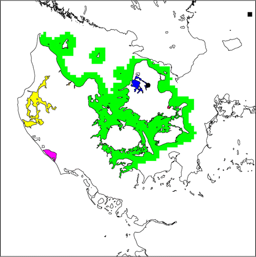
Figure 1. Subdivision for the Danish inner waters and coastal areas. Blue: Roskilde Fjord, 430 km. Green: Danish inner coast, 23,421 km. Yellow: Limfjorden, 1538 km. Orange: Mariager Fjord, 59 km. Red: Præstø Fjord, 15 km. Magenta: Rinkøbing Fjord, 206 km. The Risø site is marked with , while the BY5 site is denoted by .

In order to obtain better spatial coverage of estuaries and coastal seas than what may be obtained by measurement alone, models are developed to investigate various aspects related to biogeochemical properties of the coastal ocean, such as carbon, nutrients and pH. However, short-term variability is not always incorporated in modelling studies. Some marine models ignore short-term variability in the atmospheric concentration, when the air–sea exchange is modelled (Omstedt et al. 2009; Gypens et al., 2011; Kuznetsov and Neumann, 2013; Gustafsson et al., 2015; Valsala and Murtugudde, 2015). Similarly, when the air–sea exchange is studied from an atmospheric perspective, i.e. with atmospheric models simulating atmospheric transport and sources and sinks of , the atmospheric models tend to ignore short-term variability in surface water p and instead use monthly climatologies (Geels et al., 2007; Law et al., 2008; Tolk et al., 2009; Broquet et al., 2011; Kretschmer et al., 2014). Thus, models do not always apply the needed time resolution for simulating natural processes.

As a consequence, questions arise as to whether the estimated influence of the coastal oceans on the regional to global carbon cycle are biased, if short-term temporal variability is ignored in the parameters controlling the exchange of carbon across the air–sea interface. Often the budget is assessed on an annual scale, and short-term variability is not always included. Identifying whether important contributions are lost when ignoring high temporal variability, allows for future recommendation and improvements of models. Therefore, in this study, we systematically investigate the impact of short-term temporal variability of p on the air–sea exchange in a coastal region covering the Baltic Sea and the Danish inner waters. This systematic investigation is carried out as a model sensitivity study, where the model framework is based on an atmospheric transport model including a description of the air–sea exchange. The temporal resolution of p, in both atmosphere and surface waters, is varied over the range of monthly to sub-hourly. It is important to note that a marine process study of what drives the short-term variability in surface water p in coastal areas is not conducted here, rather we focus on investigating the impact of short-term temporal variability on carbon fluxes between atmosphere and coastal oceans. Furthermore, we examine the response of the air–sea exchange to an improved near-coastal (10 km offshore) p representation for the Danish inner waters.

2. Method

2.1. Study area

The present study focused on the Baltic Sea and the Danish inner waters. The Baltic Sea is a semi-enclosed continental shelf sea area receiving a large amount of runoff from the surrounding drainage area. This results in a low salinity outflow of surface water from the area, which in turn is ventilated by a bottom inflow of saline water from the North Sea, which passes through the narrow straits in the Danish inner waters (Bendtsen et al., 2009). Due to the vast amount of terrestrial runoff, large quantities of nutrients and terrestrial carbon are added to the Baltic Sea (Kuliński and Pempkowiak, 2011).

2.2. Surface water p

Several surface maps of p, with varying resolution in time and space, were used in the current study, in order to investigate the importance of both the spatial and temporal variability of surface water p on the air–sea exchange.

Lansø et al. (2015) created a monthly surface water p climatology for the Baltic Sea and Danish inner waters, based on a combination of observed values of p and a number of water chemistry parameters for this area. The Baltic Sea climatology (BSC) has been further developed to also include improved maps of near-coastal p for the Danish inner waters (fjord systems and straits). The coastal region of the Danish inner waters has been defined as reaching up to 10 km offshore from any Danish coastline.

These coastal p values were calculated from discrete monthly samples of alkalinity, pH, water temperature (C) and salinity (psu), using data from the Danish National Aquatic Monitoring and Assessment Program (DNAMAP, Kaas and Markager (1998)), for the period of 2000 to 2011. Calculations of p were performed using the speciation programme, CO2SYS (Lewis and Wallac, 1998), where the seawater scaled was used for pH. Cole et al. (1994) showed that the p values, calculated using this approach, have a strong and unbiased relationship with direct measurements of p (, ).

Samples from 1 m depth were used to measure alkalinity using the Danish Standards or Gran titration (Mackereth et al., 1978; Markager and Fossing, 2015. Likewise, pH were measured on samples collected at a depth of 1 m using a bleeding electrode calibrated to either pH 4 og 7 according to technical guidelines and procedures for the DNAMAP database (Kaas and Markager, 1998). Data on salinity and water temperature at 1 m were extracted from water column conductivity, temperature and depth profiles. Depending on the region, 12 to 46 samples were taken per year. For each region, data were aggregated to create monthly average values.

Six subdivisions of the Danish coastal inner water were constructed in this study. Five of these subdivisions cover individual fjords, where water chemistry has been measured, and the last subdivision is a combination of the Danish inner waters, the near-coastal area and the remaining Danish fjords (Fig. 1). Even though variations can be found within these six areas, this division was made in order to have sufficient amount of observational data to construct the climatology for the individual subdivisions. Like the original p climatology, the calculated near-coastal Danish p has been normalised to the year 2000, assuming an annual growth rate of 1.9 mol yr for in the Baltic region. A clear seasonal cycle is evident in the monthly coastal p climatology, with the highest values in winter and the lowest in spring and summer (Fig. 2). In general, the calculated near-coastal Danish p values were higher than the p values in the BSC climatology (Fig. 3).

Figure 2. Coastal Danish inner waters monthly p climatologies for the six subdivisions:

Roskilde Fjord,

Danish inner Coast,

Limfjorden,

Mariager Fjord,

Præstø Fjord,

Ringkøbing Fjord .

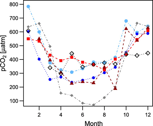
Figure 3. January and July examples of the p maps used for the Danish coastal area. Both are based on the BSC climatology. The left panels also include the improved coastal p for the Danish inner waters.

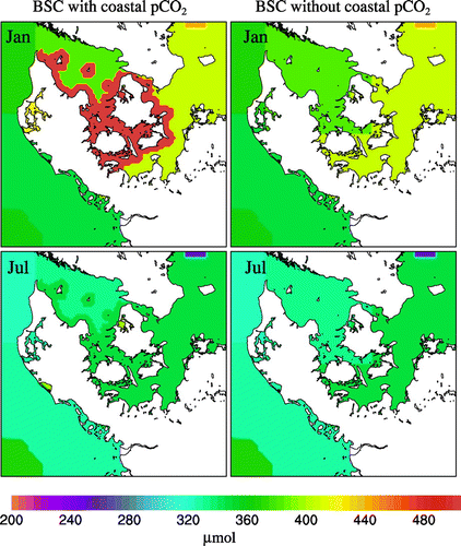
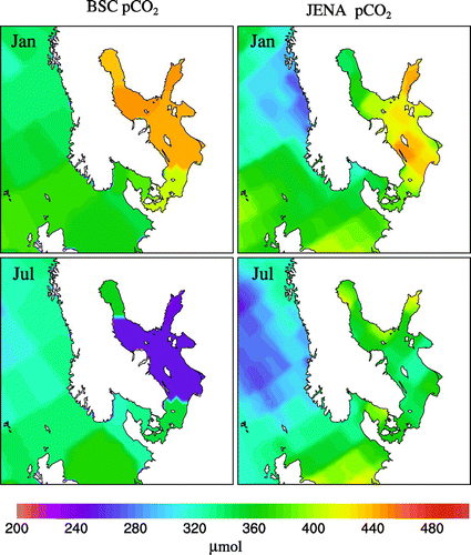
Figure 4. January and July examples of the different p maps used for the Baltic Sea. Left panel contains the BSC, while right panel contains monthly means from the JENA p surface product.

A second surface p data product, developed by Rödenbeck et al. (2013, (2014), was also applied to the current study (hereafter referred to as JENA). This product has daily fields of surface water p, on a grid resolution, from 1985 to 2012 (note the higher resolution than in the original papers). It has been constructed with the use of an observation-driven ocean mixed layer scheme, where a mixed-layer carbon budget equation, within each pixel, is used to calculate the surface p and the air–sea exchange. Hereafter, a cost function minimises the difference between the observed data points of p and the modelled data points corresponding, in space and time, to the observations. Lastly, interpolation is used for areas and times with no observational data coverage. The p observations used to constrain the modelled p have been obtained from the Surface Ocean Atlas (SOCAT), version 2 (Bakker et al., 2014).

For the study area, the same tendency for the seasonal cycle of p was observed for the BSC and JENA maps (Fig. 4, note: monthly means of p for the JENA data product have been conducted for 2011), with the highest p surface values during winter and lower values in summer. However, the seasonal amplitude of the Baltic climatology was 50-100 atm larger than JENA.

2.2.1. Temporal variability of surface water p

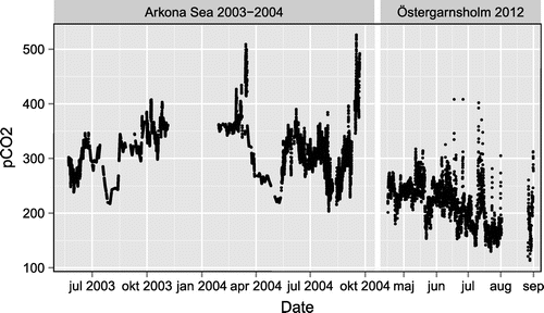
Diurnal variability of surface water p in the Baltic Sea and in the Danish waters was assessed by using the few available, continuous time series of measured surface water p, recorded at stationary sites within the Baltic Sea. It was important that the surface data was obtained from stationary sites, in order to only account for the temporal variability. Of the two sites, one is located in the Arkona Sea on a platform and the other in the Baltic Sea proper, on a small island (Östergarnsholm), off the coast of Gotland. From May 2003 to September 2004, a SAMI- sensor was deployed on a floating monitoring platform in the central Arkona Sea (54N, 1352E) at a depth of 7 m (Kuss et al., 2006). Water depth in this region is 45 m, with surface water typified by an outflow of brackish water from the Baltic Sea, while deeper water is more saline, originating from the North Sea (Weiss et al., 2007). Due to instrumental breakdown, a few data gaps are present in the time series. The Östergarnsholm site (5727N, 1859E) has been in operation since 1995. A SAMI- censor was positioned 1 km southeast of the micro-meteorological site at Östergarnsholm, at a depth of 4 m and was used in periods for continuous measurements (Rutgersson et al., 2008). Upwelling events may occur along the coast, when the wind direction is south to southwest (Norman et al., 2013a). The obtained p from Östergarnsholm spanned the period of April to August, 2012. In the two data-sets, the measured p varied between 140 and 540 atm and short-term variations, of more than 150 atm, were seen over a few days (Fig. 5). The Arkona Sea site may be seen to represent the more open water conditions of the Baltic Sea, while the Östergarnsholm site may be considered to represent more coastal conditions. From April to August the p levels at Östergarnsholm were generally lower than at Arkona Sea. This may possibly have been due to a combination of two things: inter-annual variability, as the measurements at the two sites were from different years, and the site representation of open water vs. coastal areas, as mentioned above.

Both diurnal and meso-scale variability were present in the observed time series of surface water p. These may be linked to changes in both atmospheric and marine system and processes. The focus, in this study, has been placed on the diurnal variability, with the construction of diurnal cycles of p on a monthly basis, i.e. one diurnal cycle was calculated for each month, where data existed at either of the two sites. To calculate the mean diurnal cycles, the approach as in Leinweber et al. (2009) was applied. First the mean monthly diurnal anomaly was obtained by removing a central 24 h running mean from the p time series in the month under investigation. Thereafter, the diurnal cycle was calculated by taking the mean of each hour, every day. In cases where data from the same month existed at both sites, a mean diurnal cycle was calculated from the two obtained diurnal cycles. Sufficient quantities of p were only available for eight months of the year. While no apparent diurnal variability was evident in February (Fig. 6), distinct diurnal variability was observed in the remaining months (April, May, June, July, August, September and October).

The amplitudes of the calculated diurnal cycles were much smaller than the short-term variability seen in the raw data from the two sites. Thus, the calculated monthly diurnal cycles did not capture the potentially much larger variability that may occur. Therefore, one month with a dense data coverage of measured surface p was also examined within the modelling framework. In the selected month (Arkona Sea July 2004), the actual variability of surface p showed (Fig. 7) several episodes where the p changed by more than 50 atm within a day.

2.3. Model setup

2.3.1. Modelling framework

The Danish Eulerian Hemispheric Model (DEHM) was used for the present study. The DEHM model is a three-dimensional atmospheric chemical transport model with 58 chemical species and nine classes of particulate matter (Christensen, 1997; Brandt et al., 2012). A previously developed special version of the DEHM model that only simulates atmospheric transport of has been shown to perform very well (Geels et al., 2002; Geels et al., 2004; Geels et al., 2007). It is this version of DEHM that was used and further developed in the current study. DEHM has 29 vertical layers and covers the Northern Hemisphere with a resolution of and, with increasing resolution in nests, zooms in on Europe (), Northern Europe () and Denmark (). The time step of the DEHM model meets the criteria for stability, and thus depends on both grid size and wind velocity, typically being in the range of 3–20 min.

Figure 5. Continuous measurements of surface water p from the Arkona Sea platform and the Östergarnsholm site.

The meteorological forcing used in DEHM was simulated by the Weather Research and Forecast Model (WRF) (Skamarock et al., 2005), which makes use of the same nests as the DEHM model, and uses the ERA-Interim meteorological data as the outer boundaries (Dee et al., 2011).

Surface fluxes of from NOAAs ESRL Carbon Tracker system, version CT2013b (Peters et al., 2007), were applied in the DEHM model for anthropogenic emissions, wild fire emissions and biospheric fluxes. Here, the optimised biosphere fluxes were used. Their resolution is , with updated values every three hours. However, for Europe, hourly anthropogenic emissions on a 10 km 10 km grid, from the Institute of Energy Economics and the rational Use of Energy (IER) (Pregger et al., 2007) were applied. For the nest over Denmark, these were substituted for emissions with a higher spatial resolution of 1 km 1 km (Plejdrup and Gyldenkærne, 2011). As the European and Danish emission inventories were from 2005 to 2011, the emissions were scaled to the total annual national emissions of fossil fuel and cement production as recorded by EDGAR (Olivier et al., 2014), in order to include the yearly variability in national anthropogenic emissions.

Central to this sensitivity study is the description of the air–sea exchange. In the modelling framework this was simulated by equation:(1)

where K is solubility calculated as in Weiss (1974), is the transfer velocity of normalised to a Schmidt number of 600, and is the difference in partial pressure of between the surface water and the overlying atmosphere. The transfer velocity parameterisation(2)

found by Ho et al. (2006) was used in the present study with denoting the wind speed and Sc the Schmidt number. Calculations of the air–sea exchange occurred at each modelled time step.

2.3.2. Experimental design

In order to investigate the influence of the temporal resolution of p on the air–sea exchange, various model simulations were conducted, where only the temporal resolutions of p in water and atmosphere were changed (Table 1). The temporal resolution of p in simulations with the BSC was either monthly or hourly, where the hourly resolution of the p fields was obtained by imposing the average monthly diurnal cycles onto the corresponding monthly surface field. The diurnal cycles followed the local hour in the DEHM model grids. Due to a lack of data, it was not possible to estimate average diurnal cycles representing the conditions during January, March, November and December, so values from months representing corresponding seasons were applied. Thus January, November and December used the diurnal variability from February, while data from April was used for March. The temporal resolution of atmospheric p was equal to the time step of the model, except for one simulation, where monthly means were applied.

To analyse the effect of daily p fields on the air–sea exchange, simulations with the JENA p surface product were performed. In order to isolate the effect on the air–sea exchange from the time resolution of surface water p, and disregarding the impact of different p surface products, three simulations were conducted with the JENA surface product. One had the original temporal resolution, i.e. daily, for the second simulation monthly means of surface water p from the JENA product was used, and for the last simulation the monthly diurnal cycles were imposed onto the mean daily JENA p fields. Thus, the three JENA simulations allowed for examination of the impact on the air–sea exchange from three different temporal resolutions of surface water p; monthly, daily and diurnal.

A short simulation for the month of July was conducted with real time variability of p, as observed at the Arkona Sea platform in July 2004. The hourly, real time variability was applied to each grid of the July BSC p field and followed the local hour of that specific model grid.

Furthermore, the spatial variability in near-coastal areas was also examined. The p in fjord systems, shallow and near-coastal areas can differ from p of more open waters. This effect on the air–sea exchange was investigated by conducting simulations that included or excluded the improved near-coastal p maps for Danish inner waters. The near-coastal p maps were only included in the inner nest of DEHM (with resolution of 5.6 km 5.6 km), in order to ensure the near-coastal representation. In the other nests of DEHM, the resolution was too coarse to resolve this sufficiently.

All simulations were conducted for year 2011, and model inputs were in accordance with this year.

3. Results

3.1. Temporal resolution

3.1.1. Baltic Sea climatology

Results from the 50 km -pagination 50 km nest were used to examine monthly and annual means for the Baltic Sea and Danish inner waters for the simulations vacm, vavm and cacm (Table 1), which all included the surface fields from BSC. On an annual basis, all three simulations resulted in an release of to the atmosphere for the Baltic Sea and Danish inner waters (Table 3). Comparing the results of the three simulations, using vacm as the reference, it is evident that excluding short-term variability in atmospheric p (cacm) resulted in a lower annual outgassing, while including short-term variability in the surface water p, increased the simulated outgassing by 15% from 448 GgC yr to 514 GgC yr.

A clear seasonal cycle in the air–sea exchange was present in the three simulations, with outgassing in winter and uptake during spring and summer (Table 2). The largest percentage difference between these simulations are found in the transition months between uptake and outgassing of , where atmospheric and oceanic levels of p are close to equilibrium. Differences between vacm and cacm were smallest in the summer season (May to August), and thus ignoring variability in atmospheric , has the greatest impact on the air–sea flux during winter.

Figure 6. Calculated averaged monthly diurnal cycles of surface water p.

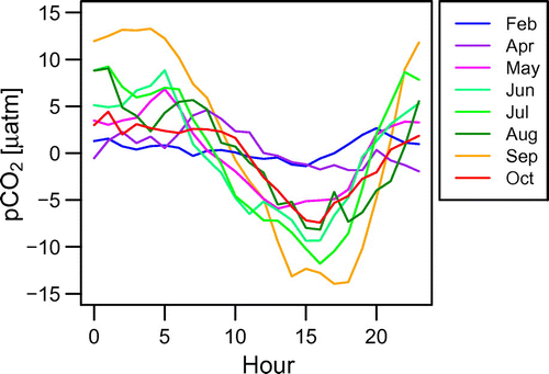
Table 1. List of simulations. Abbreviations are used for the simulation names and refer to the temporal resolution of p: v:variable, c:constant monthly, a:atmosphere, m:marine. BSC is an abbreviation of the Baltic Sea Climatology, while JENA corresponds to the surface p product developed by Rödenbeck et al. (2013) and Rödenbeck et al. (2014).

Simulation name	p map	Sea	Atmosphere
vacm	BSC	Monthly	Sub-hourly
vavm	BSC	Diurnal	Sub-hourly
cacm	BSC	Monthly	Monthly
vavm_noDK	BSC no coastal p	Diurnal	Sub-hourly
RV_vavm	Real var	Hourly	Sub-hourly
jena_mon	JENA	Monthly	Sub-hourly
jena_day	JENA	Daily	Sub-hourly.
jena_dv	JENA	Diurnal	Sub-hourly.

Time series of in both surface water and atmosphere, air–sea exchange and flux difference between simulations for January and July 2011 of the vacm, vavm and cacm runs are shown in Appendix A, Fig. A1 and Fig. A2. The time series were extracted at BY5 (5515N, 1559E), a marine monitoring site in the Baltic Proper (Fig. 1). Short temporal variability were evident in the controlling parameters of the air–sea flux, and the variations in the air–sea fluxes were clearly seen to be linked to variations in wind speed and p, with high wind speeds amplifying the air–sea flux and the differences in the flux between the simulations.

3.1.2. Real variability

For July 2011, a simulation (RV_vavm) with measured variability of surface water p was conducted for the Baltic Sea and Danish inner waters, which simulated monthly uptake for the six sub-basins within this area (Table 4). These monthly RV_vavm fluxes deviated more from vacm and vavm, than what the latter two deviated from each other. In four out of the six sub-basins, the smallest uptake is seen for RV_vavm. Thus, using RV_vavm reduce the marine uptake of atmospheric during July. Numerically, the largest changes were obtained for the Western Baltic and the Baltic Proper – the two sub-basins with the greatest area, while the largest percentage change was obtained for Kattegat. Here, the surface water p was closest to the atmospheric levels.

Figure 7. Actual variability of surface water p measured at the Arkona Sea platform during July 2004.

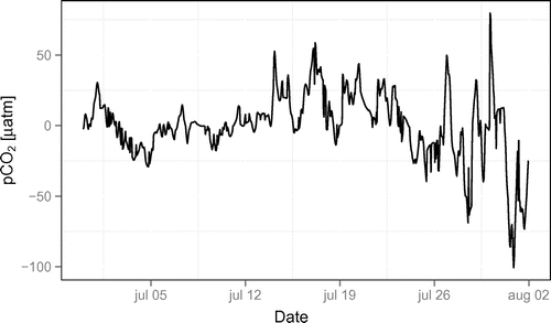
Table 2. Monthly means of the air–sea flux for the Baltic Sea and the Danish inner waters (GgC month). The last column shows the net annual flux (GgC yr). A positive sign indicates the release of from the ocean to the atmosphere, while a negative sign indicates the uptake of atmospheric by the ocean.

	Jan	Feb	Mar	Apr	May	Jun	Jul	Aug	Sep	Oct	Nov	Dec	Ann
vacm	1102	590	42	1314	2154	1336	1587	1218	47	1581	1811	3061	448
vavm	1111	598	34	1308	2153	1340	1586	1217	27	1572	1820	3079	514
cacm	1080	509	73	1334	2172	1341	1594	1227	81	1519	1735	3006	28

Table 3. Annual means, differences and percentage change for the Baltic Sea and Danish Inner waters. Annual means and differences are in GgC yr. Differences and percentage changes are calculated with vacm as the reference.

Simulation	Annual mean	Difference	Percentage
vacm	448
vavm	514	66	15
cacm	28	420	94

Table 4. July monthly means, differences and percentage change for the simulations RV_vavm, vacm and vavm for the six sub-basins within the Baltic Sea and Danish inner waters. Monthly means and differences are in GgC month. The notation of difference and percentage changes are given as vacm, and vavm when indicating the difference and percentage change with respect to RV_vavm, while vacm_vavm is between these two simulations.

	Monthly means				Differences				Percentage change
sub-basins	RV_vavm	vacm	vavm		vacm	vavm	vacm_vavm		vacm	vavm	vacm_vavm
Kattegat	29.14	32.77	32.67		3.63	3.53	0.10		11.08	10.81	0.30
Western Baltic	175.83	186.54	185.99		10.71	10.16	0.55		5.74	5.46	0.30
Baltic Proper	780.23	792.18	792.19		11.95	11.96	0.01		1.51	1.51	0.00
Gulf of Finland	79.31	78.73	78.85		0.57	0.46	0.11		0.73	0.58	0.14
Bothnian Sea	369.47	365.33	365.60		4.14	3.87	0.27		1.13	1.06	0.07
Bay of Bothnia	130.97	131.03	130.91		0.05	0.07	0.12		0.04	0.05	0.09

Short-term variability of the RV_vavm simulation was examined at the Risø site (5541N, 1205E), a coastal site in the Roskilde Fjord, Denmark (Fig. 1). The real time variability used for the surface water p resembled a diurnal cycle (Appendix A, Fig. A3) with diurnal amplitudes up to 80 atm, while the diurnal amplitude in the vavm simulation only amounted to 20 atm for July. At this coastal site, the atmospheric concentration was in phase with the marine p, with high night time values that were lowered during the day. During the growing season, this is typical behaviour for continental atmospheric concentrations, and is known as the rectifier effect (Denning et al., 1996). Boundary layer dynamics works together with plant photosynthesis to lower the atmospheric during the day, while at night together with plant respiration to increase it.

The importance of observed variability in surface water p, as compared to the diurnal cycle used in vavm, may be assessed by the air–sea flux difference between the two simulations (Appendix A, Fig. A3). This flux difference followed the pattern of p from the RV_vavm simulation, and was greatest during time periods with medium to high wind speeds. Episodes with very different surface water p between RD_vavm and vavm, but with low wind speeds, resulted in similar air–sea exchanges, again emphasising the large influence of wind speed.

3.1.3. JENA

Results from the simulations based on JENA were also analysed for the Baltic Sea and Danish inner waters. The total annual flux for the area changed by 96% and 123 %, when the temporal resolution of the surface water p was changed from monthly to daily and diurnal (Table 5). The study region changed from being an annual sink (jena_mon), to an even smaller sink close to neutral (jena_day), and then to a source (jena_dv) of atmospheric . In all three simulations, outgassing was simulated during winter and uptake was simulated from March to September. The largest differences between jena_mon and jena_day or jena_dv are obtained during the winter season when outgassing occurs. Here the release of increased by 4.0 and 4.7%, respectively.

Figure 8. The progression of surface water p during 2011 at the BY5 site for the simulations based on the JENA p product.

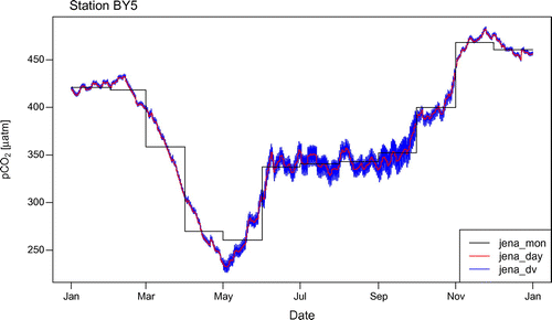
Table 5. Seasonal uptake and release, annual means, differences and percentage change in the Baltic Sea and Danish inner waters for the JENA simulations. Differences and percentage changes are calculated with jena_mon as the reference. The units are in GgC yr.

Simulation	Uptake	Release	Mean	Diff.	%
jena_mon	5187	4945	242
jena_day	5151	5142	9	233	96
jena_dv	5120	5176	56	298	123

Table 6. Annual means, differences and percentage change for the Danish coastal areas using results from nest 4 of the DEHM. Annual means and differences are in GgC yr. Differences and percentage changes are calculated with vacm as the reference.

Simulation	Annual Mean	Difference	Percentage
vacm	996
vavm	999	3	0.3
cacm	973	23	2
vavm_noDK	229	1226	123

The greatest changes in the air–sea exchange between jena_mon and jena_day/jena_dv were obtained in the periods where the surface water p changed rapidly. Annual time series of surface water p for the JENA simulations at BY5 (Fig. 8) showed that these transition periods occurred in two main periods. From February to April, the biological activity during spring resulted in the decrease of surface water p, but in May the strength of the spring bloom subsided, and the p consequently increased. In the months of October and November mineralisation take place, the effect of which results in a rapid increase in surface water p (Wesslander et al., 2010). Changes of up to 100 atm within a month and 50 atm within a week were seen for the jena_day simulation during 2011.

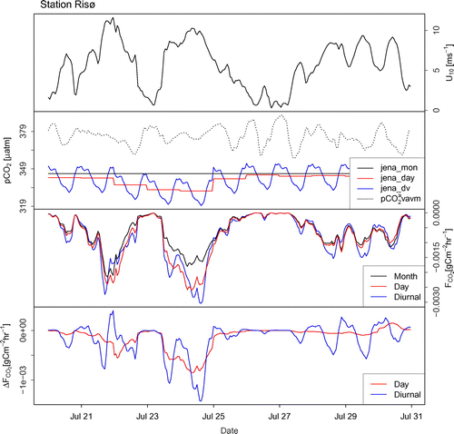
The importance of the different temporal resolutions of surface water p in the JENA simulations were clearly illustrated at the Risø site from 20 to 31 July 2011 (Appendix A, Fig. A4). During this period p of jena_day was below the monthly mean value of jena_mon, while the diurnal variability within jena_dv provided night time p values higher than the monthly mean. The different resolution of p were evident in the simulated air–sea exchange, and even further the short-term variability of jena_day and jena_dv were transferred into the flux differences of jena_mon vs. jena_day, and jena_mon vs. jena_dv.

3.2. Impact of including improved coastal p

Outputs from the inner nest of the DEHM model were used to investigate the influence of an improved near-coastal p climatology in the Danish inner waters. Air–sea fluxes for the Danish coastal inner waters, as simulated in the four different model runs using the BSC data, were compared throughout 2011. Excluding the near-coastal regions in the simulation gave significant changes in the fluxes and on an annual basis changed the region from a source to a sink (Table 6).

Table 7. Monthly mean air–sea fluxes for the Danish coastal areas for the simulation vavm, including the improved coastal p (GgC month). The last column is the annual total flux(GgC yr).

	Jan	Feb	Mar	Apr	May	Jun	Jul	Aug	Sep	Oct	Nov	Dec	Ann
Roskilde Fjord	3.89	3.88	0.01	0.50	0.66	0.23	0.23	0.25	0.68	4.54	2.68	5.97	16.82
Danish inner coast	169.26	266.81	60.77	15.38	43.13	10.59	5.12	28.36	51.50	102.01	192.65	508.73	961.52
Limfjorden	10.16	1.93	5.70	3.66	5.89	3.81	2.69	2.01	0.57	5.18	10.63	20.16	17.34
Mariager Fjord	0.07	0.14	0.05	0.10	0.11	0.10	0.08	0.10	0.08	0.05	0.14	0.24	0.04
Præstø Fjord	0.01	0.07	0.00	0.01	0.03	0.02	0.02	0.00	0.04	0.07	0.04	0.11	0.15
Ringkøbing Fjord	1.55	0.51	0.25	0.49	0.54	0.11	0.04	0.15	0.10	0.77	0.46	1.27	2.75

Table 8. Monthly mean air–sea fluxes for the Danish coastal areas for the simulation vavm, without improved coastal p (GgC month). The last column is the annual total flux(GgC yr).

	Jan	Feb	Mar	Apr	May	Jun	Jul	Aug	Sep	Oct	Nov	Dec	Ann
Roskilde Fjord	0.25	0.04	0.82	1.01	0.93	0.44	0.58	0.35	0.16	0.44	0.53	1.06	1.90
Danish inner coast	23.76	9.13	93.67	77.09	60.31	36.84	49.39	37.68	7.03	16.10	30.70	103.04	212.18
Limfjorden	0.33	2.22	2.99	2.03	2.45	2.08	1.38	1.94	1.34	1.80	1.10	1.19	12.93
Mariager Fjord	0.01	0.01	0.04	0.02	0.01	0.01	0.01	0.02	0.02	0.01	0.00	0.04	0.03
Præstø Fjord	0.01	0.00	0.01	0.03	0.02	0.01	0.01	0.01	0.01	0.01	0.01	0.02	0.04
Ringkøbing Fjord	0.32	0.51	0.32	0.36	0.51	0.32	0.35	0.33	0.40	0.54	0.48	0.72	2.47

Both with and without the near-coastal surface water p climatology a seasonal cycle in the air–sea exchange was apparent for the near-coastal Danish areas (Table 7, Table 8). In simulations, where the improved coastal p was included, the seasonal cycle of the air–sea exchange in the Danish coastal area experienced large outgassing in winter and autumn. Even during summer, outgassing was apparent, albeit to a much smaller extent, with August being an exception and showing an uptake of atmospheric . The total flux for the Danish near-coastal area was dominated by the largest coastal sub-domain (referred to as the Danish inner coast) and contributed approximately with 96 % of the estimated annual flux. In this domain, outgassing was simulated for all months except August, while the remaining fjords/sub-areas generally had uptake during spring and summer. The Roskilde Fjord takes up atmospheric from March to June, which is consistent with Eddy Covariance and Bulk fluxes measured and calculated at the Roskilde Fjord during 2012-2014 (Mørk et al., 2016).

4. Discussion

4.1. Temporal resolution and variability of surface water p

As pointed out by previous studies, biological activity is a governing parameter of the seasonal variability of surface water p in the Baltic Sea (e.g. Kuss et al. (2006); Rutgersson et al. (2008); Wesslander et al. (2010); Löffler et al. (2012); Norman et al. (2013b)). During the season of biological production (i.e. spring and summer), the consumption of has the largest impact on surface water levels of p in the Baltic Sea (Wesslander et al., 2010), while mineralisation and mixing dominates during the autumn and winter. Furthermore, the solubility effect of temperature counteracts both the mineralisation and mixing during the winter period, and the biological production during spring and summer, limiting the seasonal amplitude. The seasonal cycle of p varies within the Baltic Sea, due to the heterogeneity of the region (Rutgersson et al., 2008; Wesslander et al., 2010). The monthly and daily surface maps of p, developed and used in the present study, are in agreement with previous studies, showing similar seasonal patterns of surface water p (Fig. 4)

Diurnal variability has not previously been assessed in detail for the study area. The present study finds from April to October a clear trend in the calculated diurnal cycles of p for the Baltic Sea, with diurnal amplitudes in the range of 7 to 27 atm. The lowest p values are being recorded in the middle of the day and the highest during the night, which indicates that biological productivity and respiration also has a dominant impact on the diurnal cycles in the region (Fig. 6). However, even large short-term variations of hours to days have been noticed within the study area. Norman et al. (2013a) measured diurnal variations in surface water p of 150 atm at Östergarnsholm, in July 2005. Mørk et al. (2016) found short-term variability of 400 atm in p at Roskilde Fjord, which was measured approximately 160 m from the shore. The summer mean diurnal cycle was 180 atm for surface water p, but even during winter, a substantial diurnal cycle of 40 atm has been observed (Mørk, 2015). The monthly averaged diurnal cycles of surface water p, constructed in the present study, are much smaller than what was found for the Roskilde Fjord. However, this seems reasonable, as the Roskilde Fjord is a estuarine system and the p measurements were conducted close to the shore, while the calculated diurnal cycles of p in this study were based on data collected from the more open water areas of the Baltic Sea (Arkona Sea and Östergarnsholm). Thus, the calculated monthly averaged diurnal p cycles may be conservative estimates for some areas within the study region, particularly for the fjords and near-coastal regions.

A summer diurnal amplitude of 22 atm in surface water p was found off the Californian coast at Santa Monica Bay (Leinweber et al., 2009). As in the present study, several weeks of continuous measurements provided a solid base for their estimation of a mean diurnal cycle in p. This coastal up-welling system differs in many aspects from the Baltic Sea system. Temperature, for example, was found to have a larger influence than biology on the diurnal cycle of the surface water p at this site. As similar amplitudes of summer diurnal cycles may be obtained in different coastal systems (upwelling and marginal seas), it does not seem unreasonable that coastal seas experience a diurnal variability of 20 to 25 atm, which is much greater than the diurnal variability observed for the open ocean (DeGrandpre et al., 2004).

The actual variability applied in the RV_vavm simulation is from the Arkona Sea site, and thus represents the more open water conditions of the Baltic Sea. Continuous measurements from Östergarnsholm showed similar variability to that found at the Arkona Sea site, while those from the Roskilde Fjord showed much larger variability. It is, therefore, not unreasonable to use the actual variability found at Arkona Sea as an approximation for the entire Baltic Sea . It might, however, not be realistic to use the same variability in surface water p for the entire Baltic domain simultaneously, due to the heterogeneity of the Baltic Sea. But for the present sensitivity study, the use of actual, real variability in the entire Baltic Sea serves as an excellent method to assess the effect of including realistic short-term variability of surface water p on the air–sea exchange. A feature of the RV_vavm simulation is that variability from meso-scale systems in surface water p is also included. The monthly simulated air–sea flux shows a deviation from the simulation with the idealised calculated diurnal cycle, and reveals the importance of including short-term variability of p on both meso- and diurnal time scales.

4.2. Annual air–sea exchange

The effect of the temporal resolutions of surface water p on the annual air–sea exchange is notable for the study region. For the simulations using the BSC, the annual air–sea exchange increases by 15%, when diurnal variability in surface water p is included, resulting in a simulated larger release of to the atmosphere, for 2011. For the one month simulation using actual variability in surface water p, RV_vavm, the uptake is reduced, compared to the vacm and vavm simulations for this month. This indicates how important the implementation of realistic temporal variability in surface water p is for the air–sea exchange. Simulations using the JENA surface product indicate that a systematic bias is introduced in the annual flux of across the air–sea interface when a lower temporal resolution in the p is used. The marine area even changes from being an annual sink to a source, when the temporal resolution is increased.

Both in summer and winter positive and negative flux differences are obtained among the simulations (Appendix A, Fig. A1–A4). According to Table 2 and Table 5 the largest differences are found in the outgassing season and in particular in the transition months, where the region changes from a source to a sink and vice versa. The main hypothesis to explain this is related to the parameterisation of the transfer velocity that is non-linearly dependent on wind speed. As seen in the time series plots (Appendix A, Fig. A1–A4) the flux differences between the simulations are greatest for high wind speeds. With a tendency of higher wind speed during the winter season, the largest overall flux differences are found here, and the outgassing is amplified when the temporal resolution is increased for both BSC and JENA.

The simulations conducted in the present study show that the annual estimate of the air–sea exchange is sensitive to the temporal resolution of surface water p. Measurement studies come to similar conclusions: episodic variations of p within 30 days can impact the monthly flux estimates by 20-50% during spring and fall in the Gulf of Main (Vandemark et al., 2011), and a storm event in connection with an increase in p has been found to increase the monthly air–sea flux by 66% in the Roskilde Fjord (Mørk et al., 2016). Studying the spatiotemporal resolution in the California current system, Turi et al. (2014) noted that the existing observations for this particular area were sufficient to estimate a mean annual flux, but the observational network needed to be expanded in order to assess the variability around this mean, in time and space. Global estimates of the total coastal air–sea flux also fail to include short-term variability, in particular, due to lack of data. Laruelle et al. (2010) used annual estimates of the air–sea exchange from 62 locations, while Chen et al. (2013) included seasonality in their annual estimations. However, only 28 out of 165 estuaries are represented in all seasons, while 26 out of 87 continental shelves are represented in all seasons.

It is thought that coastal seas and estuaries have a disproportionately large effect on the global air–sea exchange. Global estimates of coastal and estuarine air–sea fluxes are still uncertain and vary from -0.19 PgC yr to -0.45 PgC yr , and 0.1 PgC yr to 0.50 PgC yr (Borges et al., 2005; Borges, 2005; Chen and Borges, 2009; Laruelle et al., 2010; Chen et al., 2013; Laruelle et al., 2014). As seen from these estimates, the air–sea flux for the total coastal area (i.e. coastal seas and estuaries) could potentially be close to zero. Including short-term variability in surface water p adds to the complexity, and is not necessarily averaged out in the estimates of the annual air–sea exchange, as shown by the current sensitivity study. Some of the uncertainties related to the flux estimates might, therefore, be minimised by including short-term variability. On the other hand, however, imposing short-term variability on surface water p introduces uncertainty, especially as short-term variability differs from site to site and continuous data from stationary sites are unable to assess the temporal variability while also validating it. Even though short-term variability in open oceans is less than that found in coastal areas, it could have an impact on the air–sea exchange and its direction for areas with p values close to the atmospheric concentration. Thus, ignoring short-term variability in open oceans could also have a potential effect on the annual global estimate of the air–sea exchange.

4.3. Atmospheric influence

Atmospheric short-term variability of was found to be averaged out and have only a limited impact on the annual air–sea exchange in the Gulf of Main (Vandemark et al., 2011). On the contrary, the present study finds that atmospheric variability has an influence on both the seasonal and annual regional fluxes for the Baltic Sea. Marine models supplying monthly atmospheric boundary conditions in coastal regions, potentially introduce a systematic bias into their flux estimates of flux across the sea surface, when they ignore short-term variability in the atmosphere.

When discussing short-term variability in relation to the air–sea exchange, it is also worth mentioning the importance of wind speed. It has an important impact on the air–sea exchange and, as seen in the present study, large deviations in p between the simulations do not necessarily result in flux differences, unless the wind speed supports it. Therefore, high spatiotemporal resolution of the wind speed should also be included in all modelling studies of the air–sea exchange.

4.4. Importance of the applied surface p

The improved surface p climatology of the near-coastal areas for the Danish inner waters shows greater seasonality than the BSC for this specific area. Only few measurements exist of measured surface water p in Danish near-coastal areas, and the calculated values of the Danish near-coastal climatology is thus difficult to certify. However, the obtained seasonal trends are undoubtedly accurate and mimics that of the Baltic Sea. Measurements of p at the Roskilde Fjord, Limfjorden and Aarhus Bay (comparable to the Danish inner coast) conducted during spring, summer and fall 2012 (Mørk, 2015), show that the calculated surface water values of p for the near-coastal areas of the Danish inner waters, in general, appear to be within the anticipated range, while the calculate spring values for the Roskilde Fjord, and the summer values for Limfjorden, seem too high. These differences are expected due to the different methods used for sampling (directly measured p vs. calculated p based on water chemistry) and time periods (one day transect measurements vs. a monthly climatology). Consistency between measured and calculated values of p was likewise found during the construction of the BSC climatology, which is partly based on measured p and calculated p (see Lansø et al. 2015).

The differences in both monthly and annual air–sea exchange for the Danish coastal areas are substantial when simulations are conducted with and without the Danish near-coastal p climatology. The change of surface water p climatology is more influential than the temporal resolution of surface water p, for this coastal area. This indicates that caution should be taken when global open ocean p is extrapolated to coastal sites, and when the air–sea exchange is assessed for these regions. This has typically been the standard in many atmospheric studies of , where the global open ocean p climatology by Takahashi et al. (2002), Takahashi et al. (2009) and Takahashi et al. (2014) is extrapolated to cover all marine areas (e.g. Geels et al., 2007; Law et al., 2008; Tolk et al., 2009; Broquet et al., 2011; Kretschmer et al., 2014).

For the entire Baltic Sea, the impact of the chosen surface p maps is also clear. The use of the BSC maps results in a simulated annual release of to the atmosphere (Table 3). For the JENA simulations only jena_dv has a small release in 2011, while jena_day is close to neutral and jena_mon shows an uptake (Table 5).

The most realistic model simulation conducted in the present study is the jena_dv. Here, the mean diurnal cycles were imposed onto the daily JENA fields, which provided a more dynamic and reasonable temporal development of surface water p than when the diurnal cycles were imposed onto the monthly fields.

However, the approach of using various maps of surface water p in the present sensitivity study is simplification of reality. A model system containing both a marine, atmospheric and biospheric components, and the coupling between them would be an improvement. Doing so, the linkage between the terrestrial biosphere and Baltic Sea could also be assessed, which for the Baltic Sea is important, as river runoff provides the majority of the dissolved organic carbon to the area (Kuliński and Pempkowiak, 2011). It would be interesting to investigate whether temporal variability in runoff affect the carbon budget of the Baltic Sea, on seasonal or interannual time scale. Such variability in runoff could arise from the impact of extreme weather, such as precipitation events (Bauer et al., 2013) or drought.

5. Conclusion

In the present study, the impact of including short-term variability in surface water p, when making annual budget estimates of air–sea exchange in coastal regions, has been explored. A model-based sensitivity study was constructed where various temporal resolutions of surface water p were applied, ranging from monthly to hourly. Three different surface maps of p were used: the BSC, the BSC with an improved coastal representation, and JENA.

Monthly mean diurnal cycles of surface water p were calculated for the Baltic Sea, based on two observed time series. No clear cycles was seen in winter, but diurnal amplitudes during the boreal summer were found to be between 7 and 27 atm, which is comparable to other coastal studies.

The monthly mean diurnal p cycles were incorporated into the modelling framework and, for the BSC, the annual air–sea exchange for the Baltic Sea and Danish inner waters increased by 15% for 2011, when the resolution of the marine p was changed from monthly to hourly (i.e. to diurnal cycles). Even larger changes in the monthly air–sea exchange were simulated when observed variability of p was imposed onto the July surface fields of surface water p, than when the monthly diurnal cycle was imposed. For the JENA simulations, an increase in the temporal resolution of the surface water p (monthly, daily and hourly) resulted in significant changes in the net yearly air–sea flux. The study area has been estimated to shift from being an annual sink to an annual source of atmospheric in the year of 2011, when the temporal resolution was increased.

The use of an improved Danish near-coastal surface water p climatology in the modelling framework resulted in a simulated annual release of to the atmosphere for the Danish near-coastal area, while excluding it resulted in an apparent annual uptake. The choice of surface p maps was found to have a crucial impact on the air–sea exchange, and better coverage of relevant surface water parameters in coastal areas is needed in order to investigate the net contribution of these areas to the regional or global carbon budget.

Despite the major impact of the chosen p fields on the annual air–sea exchange, this study also showed that the temporal resolution of surface water p is an important factor to include. Likewise, short-term variability in atmospheric p is influential, and we urge marine modellers to incorporate atmospheric variability in future studies.

In order to develop a more comprehensive picture of the temporal variability in coastal waters and its influence on carbon budget estimations, it would be interesting to couple a process-based marine model capable of simulating meso-scale dynamics in the surface waters with an atmospheric transport model. This would allow for high resolution modelling of the air–sea exchange in coastal areas, over both time and space, while also allowing for the ability to assess the impact of short-term variability on annual fluxes in greater detail.

Acknowledgements

Our utmost gratitude to Joachim Kuss, of the Leibniz Institute for Baltic Sea Research, for sharing the surface water p continuous measurements from the Arkona Sea platform. Christian Rödenbeck is appreciatively acknowledged for providing daily global maps of surface water p, for which we also extend our acknowledgement to the SOCAT data base. NOAA ERSL CarbonTracker, version CT2013B, has greatly contributed to this work, as have GLOBALVIEW-CO2, 2013, and EDGAR, IER and Aarhus University for the emissions inventories for fossil fuel emissions. Peter Stæhr and Cordula Göke at Department of Bioscience, Aarhus University, are gratefully thanked for their assistance in creating the near-coastal Danish climatology of surface water p. We are thankful for the very constructive comments from two anonymous reviewers that helped to improve and clarify the manuscript.

Additional information

Funding

This research was carried out as part of a PhD study within the Danish ECOCLIM project. This work was supported by the Danish Strategic Research Council [grant number 10-093901].

Notes

No potential conflict of interest was reported by the authors.

Appendix 1

Time series

Figure A1. January 2011 time series at the BY5 site for the simulations using the BSC. Top panel: wind speed,u applied in all the simulations. Upper middle panel: Marine p and atmospheric p, denoted pCO. Lower middle panel: air–sea exchange, . Bottom panel: Difference in air–sea exchange between the simulations, , calculated with vacm as the reference.

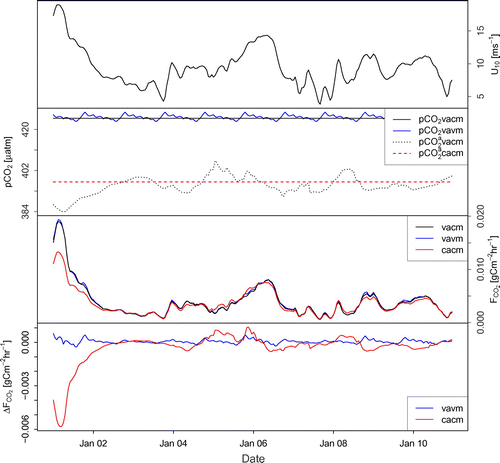
Figure A2. July 2011 time series at the BY5 site for the simulations using the BSC. Top panel: wind speed,u applied in all the simulations. Upper middle panel: Marine p and atmospheric p, denoted pCO. Lower middle panel: air–sea exchange, . Bottom panel: Difference is air–sea exchange between the simulations, , calculated with vacm as the reference.

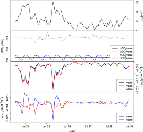
Figure A3. July time series at the Risø site for RD_vavm and vavm. Top panel: wind speed, u applied in all the simulations. Upper middle panel: Marine p and atmospheric p, denoted pCO. Lower middle panel: air–sea exchange, . Bottom panel: Difference in air–sea exchange between the simulations, , calculated as RD_vavm - vavm.

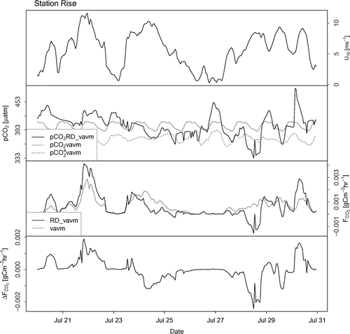
Figure A4. July time series at the Risø site for the JENA simulations. Top panel: wind speed, u applied in all the simulations. Upper middle panel: Marine p and atmospheric p, denoted pCO. Lower middle panel: air–sea exchange, . Bottom panel: Difference in air–sea exchange between the simulations, , calculated with jean_mon as the reference.

References

- Bakker, D. C. E., Pfeil, B., Smith, K., Hankin, S., Olsen, A. and co-authors 2014. An update to the Surface Ocean CO Atlas (SOCAT version 2). Earth Syst. Sci. Data 6(1), 69–90.
- Bauer, J. E., Cai, W.-J., Raymond, P. A., Bianchi, T. S., Hopkinson, C. S. and co-authors. 2013. The changing carbon cycle of the coastal ocean. Nature 504(7478), 61–70.
- Bendtsen, J., Gustafsson, K. E., Söderkvist, J. and Hansen, J. L. S. 2009. Ventilation of bottom water in the North Sea--Baltic Sea transition zone. J. Marine Syst. 75(1–2), 138–149.
- Borges, A., Delille, B. and Frankignoulle, M. 2005. Budgeting sinks and sources of CO in the coastal ocean: diversity of ecosystems counts. Geophys. Res. Lett. 32(14).
- Borges, A. V. 2005. Do we have enough pieces of the jigsaw to integrate CO fluxes in the coastal ocean? Estuaries 28(1), 3–27.
- Brandt, J., Silver, J. D., Frohn, L. M., Geels, C., Gross, A. and co-authors. 2012. An integrated model study for Europe and North America using the Danish Eulerian Hemispheric Model with focus on intercontinental transport of air pollution. Atmos. Environ. 53(SI), 156–176.
- Broquet, G., Chevallier, F., Rayner, P., Aulagnier, C., Pison, I. and co-authors. 2011. A European summertime CO biogenic flux inversion at mesoscale from continuous in situ mixing ratio measurements. J. Geophys. Res.-Atmos. 116, Article ID: D23303.
- Cai, W.-J. 2011. Estuarine and Coastal Ocean Carbon Paradox: CO Sinks or Sites of Terrestrial Carbon Incineration? Annu. Rev. Mar. Sci 3, 123–145.
- Chen, C.-T. A. and Borges, A. V. 2009. Reconciling opposing views on carbon cycling in the coastal ocean: continental shelves as sinks and near-shore ecosystems as sources of atmospheric CO. Deep Sea Res. Pt II 56(8–10), 578–590.
- Chen, C.-T. A., Huang, T.-H., Chen, Y.-C., Bai, Y., He, X. and co-authors. 2013. Air--sea exchanges of CO in the world’s coastal seas. Biogeosciences 10(10), 6509–6544.
- Christensen, J. 1997. The Danish Eulerian hemispheric model -- a three-dimensional air pollution model used for the Arctic. Atmos. Environ. 31(24), 4169–4191.
- Cole, J., Caraco, N., Kling, G. and Kratz, T. 1994. Carbon dioxide supersaturation in the surface waters of lakes. Science 265, 1568–1570.
- Crosswell, J. R., Wetz, M. S., Hales, B. and Paerl, H. W. 2012. Air-water co2 fluxes in the microtidal neuse river estuary, North Carolina. J. Geophys. Res.-Oceans 117(C8), C08017.
- Dee, D. P., Uppala, S. M., Simmons, A. J., Berrisford, P., Poli, P. and co-authors. 2011. The era-interim reanalysis: configuration and performance of the data assimilation system. Q. J. R. Meteorol. Soc. 137(656), 553–597.
- DeGrandpre, M. D., Wanninkhof, R., McGillis, W. R. and Strutton, P. G. 2004. A Lagrangian study of surface pCO dynamics in the eastern equatorial Pacific Ocean. J. Geophys. Res. Oceans 109(C8), C08S07.
- Denning, A., Randall, D., Collatz, G. and Sellers, P. 1996. Simulations of terrestrial carbon metabolism and atmospheric CO in a general circulation model 2 Simulated CO concentrations. Tellus B 48(4), 543–567.
- Gattuso, J., Frankignoulle, M. and Wollast, R. 1998. Carbon and carbonate metabolism in coastal aquatic ecosystems. Annu. Rev. Ecol. syst. 29, 405–434.
- Geels, C., Christensen, J., Hansen, A., Killsholm, S., Larsen, N. and co-authors. 2002. Modeling concentrations and fluxes of atmospheric CO in the North East Atlantic region. Phys. Chem. Earth. 26(10), 763–768.
- Geels, C., Doney, S., Dargaville, R., Brandt, J. and Christensen, J. 2004. Investigating the sources of synoptic variability in atmospheric CO measurements over the Northern Hemisphere continents: a regional model study. Tellus B 56(1), 35–50.
- Geels, C., Gloor, M., Ciais, P., Bousquet, P., Peylin, P. and co-authors. 2007. Comparing atmospheric transport models for future regional inversions over Europe - Part 1: mapping the atmospheric CO signals. Atmos. Chem. Phys. 7(13), 3461–3479.
- Gustafsson, E., Omstedt, A. and Gustafsson, B. G. 2015. The air--water CO exchange of a coastal sea -- a sensitivity study on factors that influence the absorption and outgassing of CO in the Baltic Sea. J. Geophys. Res.-Oceans 120(8), 5342–5357.
- Gypens, N., Lacroix, G., Lancelot, C. and Borges, A. V. 2011. Seasonal and inter-annual variability of air--sea fluxes and seawater carbonate chemistry in the Southern North Sea. Prog. Oceanogr. 88(1–4), 59–77.
- Ho, D. T., Law, C. S., Smith, M. J., Schlosser, P., Harvey, M. and co-author. 2006. Measurements of air--sea gas exchange at high wind speeds in the Southern Ocean: Implications for global parameterizations. Geophys. Res. Lett. 33(16), Article ID: L16611.
- Kaas, H. and Markager, S. 1998. Technical guidelines for marine monitoring. Tech. Rep. National Environmental Institute, Aarhus University, Denmark.
- Kretschmer, R., Gerbig, C., Karstens, U., Biavati, G., Vermeulen, A. and co-authors. 2014. Impact of optimized mixing heights on simulated regional atmospheric transport of CO. Atmos. Chem. Phys. 14(14), 7149–7172.
- Kuliński, K. and Pempkowiak, J. 2011. The carbon budget of the Baltic Sea. Biogeosciences 8(11), 3219–3230.
- Kuss, J., Roeder, W., Wlost, K.-P. and DeGrandpre, M. D. 2006. Time-series of surface water CO and oxygen measurements on a platform in the central Arkona Sea (Baltic Sea): seasonality of uptake and release. Mar. Chem. 101(3–4), 220–232.
- Kuznetsov, I. and Neumann, T. 2013. Simulation of carbon dynamics in the Baltic Sea with a 3D model. J. Marine Syst. 111, 167–174.
- Lansø, A. S., Bendtsen, J., Christensen, J. H., Sørensen, L. L., Chen, H. and co-authors. 2015. Sensitivity of the air--sea CO exchange in the Baltic Sea and Danish inner waters to atmospheric short-term variability. Biogeosciences 12(9), 2753–2772.
- Laruelle, G. G., Düurr, H. H., Slomp, C. P. and Borges, A. V. 2010. Evaluation of sinks and sources of CO in the global coastal ocean using a spatially-explicit typology of estuaries and continental shelves. Geophys. Res. Lett. 37, Article ID: L15607.
- Laruelle, G. G., Lauerwald, R., Pfeil, B. and Regnier, P. 2014. Regionalized global budget of the CO exchange at the air--water interface in continental shelf seas. Global Biogeochem. Cy. 28(11), 1199–1214.
- Law, R. M., Peters, W., Rödenbeck, C., Aulagnier, C., Baker, I., and\pagination{\break} co-authors. 2008. TransCom model simulations of hourly atmospheric CO: Experimental overview and diurnal cycle results for 2002. Global Biogeochem. Cy. 22(3), Article ID: GB3009.
- Leinweber, A., Gruber, N., Frenzel, H., Friederich, G. E. and Chavez, F. P. 2009. Diurnal carbon cycling in the surface ocean and lower atmosphere of Santa Monica Bay. California. Geophys. Res. Lett. 36, Article ID: L08601.
- Lewis, E. and Wallac, D. W. R. 1998. Program Developed for CO System Calculations Lab. Oak Ridge, Tenn, Technical report, Carbon dioxide Information Analysis Center, Oak Ridge Natl.
- Löffler, A., Schneider, B., Perttilä, M. and Rehder, G. 2012. Air--sea CO exchange in the Gulf of Bothnia, Baltic Sea. Cont. Shelf. Res. 37, 46–56.
- Mackereth, F., Heron, J. and Talling, J. 1978. Water analysis: some revised methods for limnologists Freshwater Biological Association.
- Markager, S. and Fossing, H. 2015. Primærproduktion. Tech. Rep. National Environmental Institute, Aarhus University.
- Mørk, E. T. 2015. Air--Sea exchange of in coastal waters. PhD thesis Aarhus University, Department of Bioscience, Denmark.
- Mørk, E. T., Sejr, M. K., Stæhr, P. A. and Sørensen, L. L. 2016. Temporal variability of air--sea exchange in a low-emission estuary. Estuar. Coast. Shelf. S. 176, 1–11.
- Norman, M., Parampil, S. R., Rutgersson, A. and Sahlée, E. 2013a. Influence of coastal upwelling on the air--sea gas exchange of in a Baltic Sea Basin. Tellus B 65, Article ID: 21831.
- Norman, M., Rutgersson, A. and Sahlée, E. 2013b. Impact of improved air--sea gas transfer velocity on fluxes and water chemistry in a Baltic Sea model. J. Marine Syst. 111, 175–188.
- Olivier, J., Janssens-Maenhout, G., Muntean, M. and Peters, J. 2014. Trends in global emissions: 2014 report PBL Netherlands Environmental Assessment Agency, The Hague.
- Omstedt, A., Gustafsson, E. and Wesslander, K. 2009. Modelling the uptake and release of carbon dioxide in the Baltic Sea surface water. Cont. Shelf. Res. 29(7), 870–885.
- Peters, W., Jacobson, A., Sweeney, C., Andrews, A., Conway, T. and co-authors. 2007. An atmospheric perspective on North American carbon dioxide exchange: CarbonTracker. PNAS 104, 18925–18930.
- Plejdrup, M. and Gyldenkærne, S. 2011. Spatial distribution of emissions to air - te spread model. Rep. National Environmental Institute, Aarhus University.
- Pregger, T., Scholz, Y. and Friedrich, R. 2007. Documentation of the Anthropogenic GHG Emission Data for Europe Provided in the Frame of CarboEurope and CarboEurope IP. Rep. University of Stuttgart, IER -- Institute of Energy Economics and the Rational Use of Energy.
- Regnier, P., Friedlingstein, P., Ciais, P., Mackenzie, F. T., Gruber, N., and co-authors. 2013. Anthropogenic perturbation of the carbon fluxes from land to ocean. Nat. Geosci. 6(8), 597–607.
- Rödenbeck, C., Bakker, D. C. E., Metzl, N., Olsen, A., Sabine, C. and co-authors. 2014. Interannual sea--air CO flux variability from an observation-driven ocean mixed-layer scheme. Biogeosciences 11(17), 4599–4613.
- Rödenbeck, C., Keeling, R. F., Bakker, D. C. E., Metzl, N., Olsen, A. and co-authors. 2013. Global surface-ocean pCO and sea--air CO flux variability from an observation-driven ocean mixed-layer scheme. Ocean Sci. 9(2), 193–216.
- Rutgersson, A., Norman, M., Schneider, B., Pettersson, H. and Sahlée, E. 2008. The annual cycle of carbon dioxide and parameters influencing the air--sea carbon exchange in the Baltic proper. J. Marine Syst. 74(1–2), 381–394.
- Skamarock, W. C., Klemp, J. B., Dudhia, J., Gill, D. O., Barker, D. M. and co-authors. 2005. A Description of the Advanced Research WRF Version 2 Report, NCAR.
- Takahashi, T., Sutherland, S., Chipman, D., Goddard, J., Ho, C. and co-authors. 2014. Climatological distributions of pH, p, total , alkalinity, and CaCO3 saturation in the global surface ocean, and temporal changes at selected locations. Mar. Chem. 164, 95–125.
- Takahashi, T., Sutherland, S. C., Sweeney, C., Poisson, A., Metzl, N. and co-authors. 2002. Global sea--air flux based on climatological surface ocean p, and seasonal biological and temperature effects. Deep-Sea Res. Pt. II 49(9–10), 1601–1622.
- Takahashi, T., Sutherland, S. C., Wanninkhof, R., Sweeney, C., Feely, R. A. and co-authors. 2009. Climatological mean and decadal change in surface ocean p, and net sea--air flux over the global oceans. Deep-Sea Res. Pt. II 56(8–10), 554–577.
- Tolk, L. F., Peters, W., Meesters, A. G. C. A., Groenendijk, M., Vermeulen, A. T. and co-authors. 2009. Modelling regional scale surface fluxes, meteorology and mixing ratios for the Cabauw tower in the Netherlands. Biogeosciences 6(10), 2265–2280.
- Turi, G., Lachkar, Z. and Gruber, N. 2014. Spatiotemporal variability and drivers of pCO and air--sea CO fluxes in the California Current System: an eddy-resolving modeling study. Biogeosciences 11(3), 671–690.
- Valsala, V. and Murtugudde, R. 2015. Mesoscale and intraseasonal air-sea exchanges in the western Arabian Sea during boreal summer. Deep-Sea Res. Pt. I 103, 101–113.
- Vandemark, D., Salisbury, J. E., Hunt, C. W., Shellito, S. M., Irish, J. D. and co-authors. 2011. Temporal and spatial dynamics of air--sea flux in the Gulf of Maine. J. Geophys. Res.-Oceans 116(C1), C01012.
- Weiss, A., Kuss, J., Peters, G. and Schneider, B. 2007. Evaluating transfer velocity--wind speed relationship using a long-term series of direct eddy correlation flux measurements. J. Marine Syst. 66(1–4), 130–139.
- Weiss, R. F. 1974. Carbon dioxide in seawater: the solubility of non-ideal gas. Mar. Chem 2, 203–215.
- Wesslander, K., Omstedt, A. and Schneider, B. 2010. Inter-annual and seasonal variations in the air--sea balance in the central Baltic Sea and the Kattegat. Cont. Shelf. Res. 30(14), 1511–1521.