Sensitivity assessment of PM_2.5 simulation to the below-cloud washout schemes in an atmospheric chemical transport model

Abstract

This study analyses the sensitivity of PM_2.5 simulation and source apportionment results by integrating different below-cloud washout (BCW) schemes from various models into the CAMx model during the rainy days (3–13 September 2010). Furthermore, this study has also considered the influence of different raindrop size distribution parameterizations on the simulation. PM_2.5 time series, spatial maps and the average concentration of the study region using different BCW schemes are presented. Our results show that different BCW schemes can cause over 50 μg m⁻³ discrepancies in a PM_2.5 simulation during the heavy rain periods. The source apportionment (, and ) results for some cities (e.g. Hong Kong) are also sensitive to the choice of the BCW scheme. After implementing the composition dependent BCW coefficients calculated by using the field observation data, the PM_2.5 simulation performance was improved and mean bias was reduced to 0.5 μg m⁻³ during the study period. Future BCW studies should focus on the effects caused by aerosol compositions and raindrop size distributions in order to produce reliable simulation results for the rainy season.

Keywords:

• precipitation
• below-cloud washout
• raindrop parameterization
• CAMx model
• PM2.5

1. Introduction

PM_2.5 (fine particulate matter), composed of primary and secondary constituents, is one of the major air pollutants that can exert adverse health effects on human beings. The gas-phase precursors of PM_2.5 come from both anthropogenic and biogenic emissions. Wet deposition and dry depositions are the two important natural sinks for this ambient pollutant in our environment. During the wet deposition process, the aerosol particles are incorporated into the hydrometeors and then transported down to the ground. The size of the particle influences the wet deposition rate and the difference can reach up to several orders of magnitude (Zhang and Vet, 2006). Wet deposition can be classified into in-cloud rainout and BCW processes. In-cloud rainout represents the process by which aerosol in the cloud is removed by rain and snow events within the cloud, which includes the activation of cloud condensation nuclei (CCN) under super-saturation condition. When precipitation event occurs, the conversion of cloud droplets to raindrops will take place and aerosol will then be removed with the rainout process. When the hydrometeors fall, the aerosol can also be captured by snow particles or rain droplets via Brownian diffusion, interception and initial impaction; this removal process is known as the below-cloud washout (BCW) (Seinfeld and Pandis, 2006; Wang et al., 2010; Duhanyan and Roustan, 2011; Zhang et al. 2013). In the past several decades, many studies have been carried out to study this process from field measurement (Laakso et al. 2003; Zikova and Zdimal, 2016), laboratory experiment (Lemaitre et al. 2017) and mathematical derivation (Kang et al. 2015). During the early stage of a rain event, the BCW process is the major contributor for the concentration of the chemical species in the rainwater; while in the later stage, the rainout process contributes substantial part of chemical species concentration in the rainwater because most of the ambient aerosol particles below the cloud base have already been removed by washout process (Chatterjee et al., 2010). These two processes may have different impacts on the various aerosol species, for instance, Aikawa et al. (2014) reported that both rainout and washout processes contributed the same for the sulphate removal; while rainout process only contributed around 33% of nitrate removal during the rain events.

Both the in-cloud rainout and BCW processes for PM_2.5 have been modelled and incorporated into many 3-D chemical transport models (CTMs) (Gong et al., 2011). Many studies have applied 3-D CTMs to study the wet deposition of particulate species (e.g., , and ) around the world. For example, Appel et al. (2011) assessed the Community Multiscale Air Quality Model (CMAQ) v4.7 , and wet deposition simulation performance in the United States. Han et al. (2006) applied a regional air quality model (RAQM) to simulate the wet deposition of , , and Ca²⁺ in East Asia. Lu et al. (2015) applied CMAQ v5.0 to simulate the and wet deposition in southern China and applied the Integrated Source Apportionment Method (ISAM) (Kwok et al., 2013) to track the sources of these two pollutants in rainwater. Hence, the simulation accuracy of the wet removal process is of great importance when 3 D CTMs are used to analyse air quality, climate, and ambient pollutant exposure topics.

Facing various parameterization methods for BCW coefficients, it is of great importance to study the sensitivity of the coefficient calculation on PM_2.5 concentration by using different methods. Wang et al. (2010) and Duhanyan and Roustan (2011) gave detailed reviews of the uncertainty of BCW coefficient calculation using different methods, raindrop size distributions, raindrop diameters, and raindrop terminal velocities. Wang et al. (2014a) showed that the magnitude of the BCW coefficient reported by different studies ranged from 10⁻⁷ to 10⁻⁴. Rasch et al. (2000) compared the model uncertainty caused by the deposition process. Recently, Gong et al. (2011) analyzed the PM_2.5 simulation sensitivity caused by different BCW schemes. They reported that the difference of simulated daily PM_2.5 concentration caused by two different BCW schemes reached 10% in a case study. In this study, we integrated the BCW coefficient calculation schemes from different 3-D CTMs (e.g., CMAQ, European Monitoring and Evaluation Programme (EMEP), and Atmospheric Dispersion Modeling System (ADMS)) into the Comprehensive Air Quality Model with Extensions (CAMx) and compared the ambient PM_2.5 simulations. CAMx is an open-source modelling system that has been applied in many studies to examine ambient pollution simulation and source apportionment (Li et al., 2012; Wang et al., 2014b; Lu et al., 2016). We also compare the simulated PM_2.5 concentration when implementing different raindrop size distributions into the CAMx model. In addition to the surface ambient PM_2.5 concentration, the sensitivity of the PM_2.5 source apportionment results (local, regional and super-regional sources) based on different parametric schemes has been analysed. We used observation data (, and composition data) to calculate the BCW coefficients for different aerosol species and investigated how the compositions influence the model simulation performance. Located in southern China, the yearly average precipitation in the Pearl River Delta region (PRD) of southern China can reach up to 1500 mm (a yearly average of 600 mm for China) and the PM_2.5 simulation performance in this region should be relevant to the BCW calculation during the rainy seasons. Therefore, we chose this region to carry out the BCW sensitivity study. Section 2 introduces the different BCW parametric schemes and CAMx model domain setting. In Section 3, we compare the ambient PM_2.5 simulations and source apportionment results when applying different BCW parametric schemes. The self-calculated BCW coefficients are also discussed in this section. A discussion and summary of this study are presented in Sections 4 and Section 5, respectively.

2. Methods

2.1 BCW calculation schemes

During rainy periods, the below-cloud removal process is directly proportional to the concentration and can be expressed by Equation (1)(1) $$\frac{dc}{dt}=-\lambda c$$(1) : (1) $$\frac{dc}{dt}=-\lambda c$$(1) where c is the ambient pollutant concentration (μg m⁻³), t is the time and λ is the scavenging coefficient (s⁻¹). Several methods that can be used to parameterize the λ value. One method is to parameterize this value by considering the collection efficiency, the diameters of both the particulate matter and hydrometeor and the particle size distribution, as shown in Equation (2)(2) $$\lambda (d_a)=\frac{\pi }{4}{\displaystyle \int D^{2}V(D)E(D,d_a)N(D)dD}$$(2) (Seinfeld and Pandis, 2006): (2) $$\lambda (d_a)=\frac{\pi }{4}{\displaystyle \int D^{2}V(D)E(D,d_a)N(D)dD}$$(2) where D represents the raindrop diameter (m), d_a is the aerosol diameter (m), V(D) is the raindrop terminal velocity (ms⁻¹), E(D,d_a) is the collection efficiency determined by the diameters of the particle and raindrop, N(D) is the raindrop size distribution (m⁻⁴). Raindrop diameter, raindrop size distribution, and particle collection efficiency can have various parameterization schemes and hence derive different values for the BCW coefficient (Duhanyan and Roustan, 2011).

In the field campaign (Laakso et al., 2003), the BCW coefficient can be calculated using Equation (3)(3) $$\lambda (d_a)=-\frac{1}{t_1-t_0}\ln \left[\frac{c_1(d_a)}{c_0(d_a)}\right]$$(3) (the integrated form of Equation (1)(1) $$\frac{dc}{dt}=-\lambda c$$(1) ): (3) $$\lambda (d_a)=-\frac{1}{t_1-t_0}\ln \left[\frac{c_1(d_a)}{c_0(d_a)}\right]$$(3) where c₁ and c₀ represent the particle concentration at time t₁ and t₀. Laakso et al. (2003) used this method to derive the scavenging coefficients for the particles with a diameters between 10 and 510 nm based on their field campaign measurement. The scavenging coefficient is dependent on different rain intensities; hence, the coefficient can be alternately parameterized by Equation (4)(4) $$\lambda (d_a)=a{P}^b$$(4) : (4) $$\lambda (d_a)=a{P}^b$$(4) where P is the rain intensity (mm h⁻¹), a and b are the constant coefficients derived from the regression relation between the λ(d_a) and P (introduced in Wang et al. (2014a)). Other scavenging coefficient expressions have also been listed in Table S1.

As one of the major ambient PM_2.5 sinks, the BCW coefficient calculation schemes in different 3-D CTMs are not the same (Gong et al., 2011). In CAMx v6.00, the BCW coefficient is calculated using Equation (5)(5) $$\lambda =4.2\times {10}^{-7}\frac{EP}{D}$$(5) : (5) $$\lambda =4.2\times {10}^{-7}\frac{EP}{D}$$(5) where λ is the scavenging coefficient (s⁻¹), E is the collection efficiency, P is the precipitation rate in mm h⁻¹, and D is the raindrop diameter (in m). The raindrop diameter and collection efficiency are calculated using Equation (6)(6) $$D=9.0\times {10}^{-4}{P}^{0.21}$$(6) (Atlas, 1953) and Equation (7)(7) $$E=\frac{4}{\mathrm{Re}Sc}[1+0.4{\mathrm{Re}}^{1/2}{S}_c{}^{1/3}+0.16{\mathrm{Re}}^{1/2}{S}_c{}^{1/2}]+4\varphi [\frac{\mu }{{\mu }_w}+\varphi (1+2{\mathrm{Re}}^{1/2})]+{\left(\frac{S_t-S^{*}}{S_t-S^{*}+2/3}\right)}^{3/2}$$(7) (Slinn, 1983) based on experiment and theoretical calculation, respectively: (6) $$D=9.0\times {10}^{-4}{P}^{0.21}$$(6) (7) $$E=\frac{4}{\mathrm{Re}Sc}[1+0.4{\mathrm{Re}}^{1/2}{S}_c{}^{1/3}+0.16{\mathrm{Re}}^{1/2}{S}_c{}^{1/2}]+4\varphi [\frac{\mu }{{\mu }_w}+\varphi (1+2{\mathrm{Re}}^{1/2})]+{\left(\frac{S_t-S^{*}}{S_t-S^{*}+2/3}\right)}^{3/2}$$(7) where $\mathrm{Re}$ is the Reynolds number for the raindrop, calculated by $\mathrm{Re}=\frac{D{V}_d}{2{\mu }_a}$ (V_d is the raindrop terminal speed (m s⁻¹), ${\mu }_a$is the air molecular diffusivity (m² s⁻¹), D is the raindrop diameter (m)); S_c is the Schmidt number, calculated by $S_c={\mu }_a/D_b$(D_b is the particle Brownian diffusivity (m² s⁻¹)); $S^{*}=\frac{1.2+\ln (1+\mathrm{Re})/12}{1+\ln (1+\mathrm{Re})}$ and S_t is the Stokes number; $\varphi$ is the ratio of particle size to the raindrop size, $\mu$ is the kinematics viscosity of air (kg m⁻¹ s⁻¹) and ${\mu }_w$ is the kinematics viscosity of water (kg m⁻¹ s⁻¹).

Theoretically, the raindrop diameter should be size-resolved to better simulate the realistic condition. However, due to the computation efficiency issue, most 3-D CTMs (e.g., CAMx and Unified Regional Air-Quality Modelling System [AURAMS]) apply the monodisperse method scaled by precipitation intensity to calculate the raindrop diameter (Wang et al., 2010). The collection efficiency calculation in the CAMx model is taken from Seinfeld and Pandis. (based on Equation (7)(7) $$E=\frac{4}{\mathrm{Re}Sc}[1+0.4{\mathrm{Re}}^{1/2}{S}_c{}^{1/3}+0.16{\mathrm{Re}}^{1/2}{S}_c{}^{1/2}]+4\varphi [\frac{\mu }{{\mu }_w}+\varphi (1+2{\mathrm{Re}}^{1/2})]+{\left(\frac{S_t-S^{*}}{S_t-S^{*}+2/3}\right)}^{3/2}$$(7) ), considering Brownian diffusion, interception and impaction. Information about the particle diameter, raindrop terminal velocity and raindrop diameter is needed to calculate the collection efficiency. CAMx v6.40 (updated in December, 2016) has made a major revision to the wet deposition algorithm. The PM_2.5 diameter is multiplied by a factor of 10 before entering the BCW calculation process to improve the scavenging of fine particles during the rain events. The last term of Equation (7)(7) $$E=\frac{4}{\mathrm{Re}Sc}[1+0.4{\mathrm{Re}}^{1/2}{S}_c{}^{1/3}+0.16{\mathrm{Re}}^{1/2}{S}_c{}^{1/2}]+4\varphi [\frac{\mu }{{\mu }_w}+\varphi (1+2{\mathrm{Re}}^{1/2})]+{\left(\frac{S_t-S^{*}}{S_t-S^{*}+2/3}\right)}^{3/2}$$(7) has also been scaled by the square root of the ratio of the water density to particle density (Seinfeld and Pandis, 2006). For more details about the BCW calculation in the CAMx model, please refer to Section 4.5 in the CAMx user manual (http://www.camx.com/files/camxusersguide_v6-40.pdf) and CAMx v6.40 release notes (http://www.camx.com/download/default.aspx).

The particle wet removal calculation process is modelled in a completely different way in the CMAQ model. In CMAQ, the precipitation scavenging process does not separate the BCW and in-cloud rainout process and treat the overall washout process in a 1-D column cloud model. The scavenging coefficient (below-cloud and in-cloud) in CMAQ for each layer is calculated using the following two equations (Roselle and Binkowski, 1999): (8) $$\alpha =\frac{1}{{\tau }_{washout}}$$(8) (9) $${\tau }_{washout}=\frac{{\overline{W}}_T\Delta z}{{\rho }_w{P}_{}}$$(9) where $\alpha$ is the scavenging coefficient (s⁻¹), ${\tau }_{washout}$ is the cloud time scale (s), ${\overline{W}}_T$ is the mean total water content at the specific layer (kg m⁻³), $\Delta z$ is the thickness of the specific model layer (m), ${\rho }_w$ is the water density (kg m⁻³), and $P$ is the precipitation rate (m s⁻¹). According to Roselle and Binkowski (1999), the accumulation mode and coarse mode aerosols are assumed to be fully absorbed by the rainwater in CMAQ, which neglects the BCW physical interactions considered in the CAMx model. The resolved cloud module of CMAQ read the total precipitation amount calculated by the Weather Research Forecast (WRF) model and separated it into each individual model vertical layer by the ratio of water content (e.g., cloud water, rainwater, and graupel water) at the specific layer to the total water content in the vertical column.

Other schemes are analysed here in addition to the two wet removal schemes (CAMx and CMAQ) described previously. The EMEP model is used widely in European countries to study air pollution issue (Simpson et al., 2012), and the BCW rate for particles in EMEP is calculated by the following equation (Scott, 1979): (10) $$\lambda =\frac{A{P}_r}{V}E$$(10) where A is 5.2 m³ kg⁻¹ s⁻² (an empirical coefficient), P_r is the precipitation rate (kgm⁻² s⁻¹), V is the raindrop terminal speed (set to be 5 ms⁻¹), and $E$ is the collection efficiency from a look-up table (Simpson et al., 2012). CALPUFF (puff dispersion model) is another advanced non-steady-state air quality model that is preferred for simulation of the long range transport of ambient pollutants. In CALPUFF, the scavenging coefficient is set as a constant (10⁻⁴s⁻¹) multiplied by the rain rate (mm h⁻¹), for sulphate and nitrate particles (Scire et al., 2000). The ADMS (Atmospheric Dispersion Modelling System) is an advanced atmospheric pollution dispersion model for calculating concentrations of atmospheric pollutants emitted both continuously from point, line, volume, and area sources. It was developed by Cambridge Environmental Research Consultants (CERC) of the United Kingdom. In the ADMS, the scavenging coefficient is expressed in the form of Equation (4)(4) $$\lambda (d_a)=a{P}^b$$(4) and the default coefficients a and b are equal to 10⁻⁴ and 0.64 (based on field measurement), respectively. The methods in the form of Equation (4)(4) $$\lambda (d_a)=a{P}^b$$(4) (parameterized by rain rate and empirical coefficients) proposed by Sparmacher et al. (1993), Baklanov and Sorensen (2001), and Wang et al. (2014c) are also compared in this study.

Three other studies have also been included for the simulation comparison. Kang et al. (2015) found that the particle collection efficiency by raindrop was proportional to Pe ^−0.5 (the Peclet number) and reported that the interception was negligible. Laakso et al. (2003) applied 6 years of field measurement data to parameterize the scavenging coefficient and analysed its dependence on rain intensity was also analyzed in their study. Loosmore and Cederwall. (2004) proposed that when the rain rate was larger than 25 mm h⁻¹, the aerosol greater than 0.2 μm in diameter was treated the same as the 10-μm particle.

2.2 Parameterization of raindrop size distribution

Based on Equations (5)(5) $$\lambda =4.2\times {10}^{-7}\frac{EP}{D}$$(5) , (6)(6) $$D=9.0\times {10}^{-4}{P}^{0.21}$$(6) , and (7)(7) $$E=\frac{4}{\mathrm{Re}Sc}[1+0.4{\mathrm{Re}}^{1/2}{S}_c{}^{1/3}+0.16{\mathrm{Re}}^{1/2}{S}_c{}^{1/2}]+4\varphi [\frac{\mu }{{\mu }_w}+\varphi (1+2{\mathrm{Re}}^{1/2})]+{\left(\frac{S_t-S^{*}}{S_t-S^{*}+2/3}\right)}^{3/2}$$(7) , the BCW coefficient calculation in CAMx is dependent on the rain rate, collection efficiency and raindrop diameter. However, based on Wang et al. (2010) and Duhanyan and Roustan (2011), the sensitivity between different expressions of monodisperse raindrop diameter and terminal velocity is limited. Hence, in this study, we only compared the simulation sensitivity caused by different raindrop size distributions.

The computational burden in 3-D CTM can be effectively decreased by using the monodisperse raindrop diameter. However, this method assumes that all raindrops have the same diameter when the rain rate is the same and it is only correct for specific raindrop spectra (Wang et al., 2010). Hence, it is closer to the real condition when the raindrop diameter is quantified with the distribution. In this study, an explicit integration of Equation (2)(2) $$\lambda (d_a)=\frac{\pi }{4}{\displaystyle \int D^{2}V(D)E(D,d_a)N(D)dD}$$(2) for the BCW coefficient calculation is modified for the CAMx model. The raindrop number size distribution we analyse includes exponential distribution, gamma distribution and log-normal distribution (listed in Table 1). We use the trapezoidal rule to perform the integration.

Table 1. Raindrop size distributions extracted from the literature.

	References	Formula
A	Marshall and Palmer (1948)^a^,1	N0 = 8$\times$10^6, $\alpha$ = 0, $\gamma$ = 1,$\beta$ = 4100P^−0.21
B	Ulbrich (1983)^a^,1	N0 = 5.1$\times$10^6P^−0.03, $\alpha$ = 0, $\gamma$ = 1, $\beta$ = 3800P^−0.2
C	Cerro et al. (1997)^a^,1	N0 = 2.32$\times$10^6P^0.22, $\alpha$ = 0, $\gamma$ = 1, $\beta$ = 4000P^−0.1065
D	De Wolf (2001)^a^,1	N0 = 1.22$\times$10^1^6P^−0.384, $\alpha$ = 2.93, $\gamma$ = 1, $\beta$ = 5380P^−0.186
E	Chapon et al. (2008)^a^,1	N0 = 7.5$\times$10^1^8P^0.001, $\alpha$ = 3.47, $\gamma$ = 1, $\beta$ = 7640P^−0.214
F	Chen et al. (2013)^a^,2	N0 = 2.1$\times$10^4, $\alpha$ = 3.51, $\gamma$ = 1, $\beta$ = 4.52
G	Aoki et al. (2016)^a^,2	N0 = 8.3$\times$10^3, $\alpha$ = 2.3, $\gamma$ = 1, $\beta$ = 3.2
H	Das et al. (2017)^a^,2	N0 = 3.16$\times$10^6, $\alpha$ = 7.9, $\gamma$ = 1, $\beta$ = 9.9
I	Chen et al. (2017)^a^,2	N0 = 610, $\alpha$ = −0.158, $\gamma$ = 1, $\beta$ = 2.26
J	Feingold and Levin (1986)^b	Ntot = 1.72$\times$10^2P^0.22, Dmean = 7.2$\times$10^−4P^−0.23, ${\sigma }_D$ = 1.43–3$\times$10^−4P
K	Timothy et al. (2002)^b	Ntot = 2.03$\times$10^2P^0.241, Dmean = e^−0.313 + 0.227ln^P$\times$10^−3, ${\sigma }_D$ = $e^{\sqrt{0.108-0.0086\ln P}}$
L	Harikumar et al. (2010)^b	Ntot = 2.68$\times$10^2P^0.308, Dmean = 5.96$\times$10^−4P^−0.216, ${\sigma }_D$ = 1.55–0.0217lnP

^a Gamma distribution: $N(D)=N_0{D}^{\alpha }\exp (-\beta D^{\gamma })$. When $\alpha$ = 0, $\gamma$ = 1, the equation then becomes the exponential distribution.

¹ N₀ unit is in m⁻³ m^−1-α, β unit is in m^−γ.

² N₀ unit is in m⁻³ mm^−1-α, β unit is in mm^−γ.

^b Log-normal distribution: $N(D)=\frac{N_{tot}}{\sqrt{2\pi }D\ln ({\sigma }_D)}\exp \left[-\frac{{(\ln (D)-\ln (D_{mean}))}^2}{2{(\ln ({\sigma }_D))}^2}\right]$. N_tot is in m⁻³, D_mean is in m.

2.3 WRF-CAMx setting

The meteorological field considered in this study was simulated by WRF ARW (Advanced Research WRF) version 3.2 and the domain setting in addition to the physical scheme selection following Lu et al. (2016). In brief, the rapid radiative transfer model longwave radiation scheme (Mlawer et al., 1997), Dudhia's (1989) shortwave radiation scheme, Yonsei University PBL scheme (Hong et al., 2006), the Noah landesurface model (Chen and Dudhia, 2001), the WRF single-moment 6-class scheme (Dudhia et al., 2008) for microphysics, and the Grelle-Devenyi ensemble cumulus parameterization scheme (Grell and Devenyi, 2002) are used for the meteorology simulation. Three nested meshes were set for this study and the domain extent (represented by the dashed line for WRF) is shown in Fig. 1. The resolutions for the largest, second and finest domains are 27 km, 9 km and 3 km, respectively. The 27-km domain covers most part of China, India, Japan, Korea and some Southeast Asian countries. The 9-km domain covers the Guangdong Province and the finest domain covers all 10 major cities in the Pearl River Delta (PRD) region. We focus on analysing the simulated results with 3-km domain only (21.54°N - 24.57°N, 111.15°E - 115.65°E).

Fig. 1. (a–c): WRF (dash line) and CAMx (solid line) domain setting. Blue dots and red numbers represent the locations of the ground-based PM2.5 observation station and precipitation observation station, respectively. ‘SZ’ represents Shenzhen, ‘HK’ represents Hong Kong, ‘HZ’ represents Huizhou, ‘DG’ represents Dongguan, ‘ZS’ represents Zhongshan, ‘ZH’ represents Zhuhai, ‘JM’ represents Jiangmen, ‘ZQ’ represents Zhaoqing, ‘GZ’ represents Guangzhou, and ‘FS’ represents Foshan.

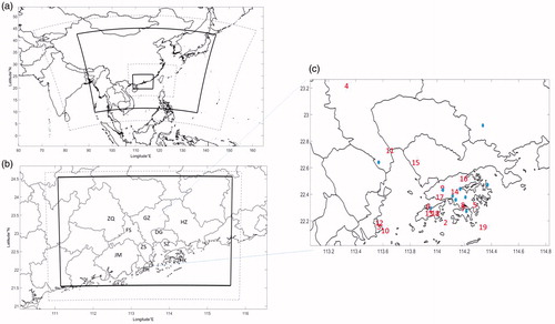
The CAMx model domain coverage is represented by the solid line in Fig. 1. In CAMx, CB05 (Carbon Bond Mechanism 05) and RADM (Regional Acid Deposition Model) were selected for gas-phase chemistry and aqueous-phase chemistry schemes. The inorganic aerosol and secondary organic aerosol modules are ISORROPIA 1.7 (Nenes et al., 1998) and SOAP, respectively. We selected the coarse/fine aerosol chemistry scheme (CF) and used the K-theory for the vertical diffusion simulation, and the Euler Backward Iterative (EBI) served as the chemical solver. The base model was CAMx v6.00 and we changed the source code of the wet deposition module based on different schemes (including CAMx v6.40) and size distribution for the comparison. We used INTEX-B (Zhang et al., 2009) emission inventory (including SO₂, NO_x, CO, VOC, PM, BC and OC) for the 27-km and 9-km domains. A resolved local emission inventory (Zheng et al., 2009) is used for the simulation in the 3-km domain. We used the Model of Gases and Aerosols from Nature (MEGAN v2.04) (Guenther et al., 2006) for biogenic emission generation. The spatial map of the emissions used in this study can be found in Lu et al. (2015).

In addition to the surface PM_2.5 simulation, the sensitivity of the source apportionment results is analysed in this study. The CTM-based source apportionment method is an important tool for pollution control policy design (Wu et al., 2013). Therefore, it is necessary to evaluate its sensitivity due to the BCW schemes during the rainy days. Particulate source apportionment technology (PSAT) was used to calculate the super-regional (outside the PRD), regional (from other cities in the PRD) and local (within the city) contributions to ambient PM_2.5 in the 10 cities in the PRD region. The PSAT in CAMx is only supported for the CF aerosol option in the current version. The BCW schemes from CAMx v6.00, CAMx v6.40, ADMS, EMEP and CALPUFF are used for the sensitivity comparison.

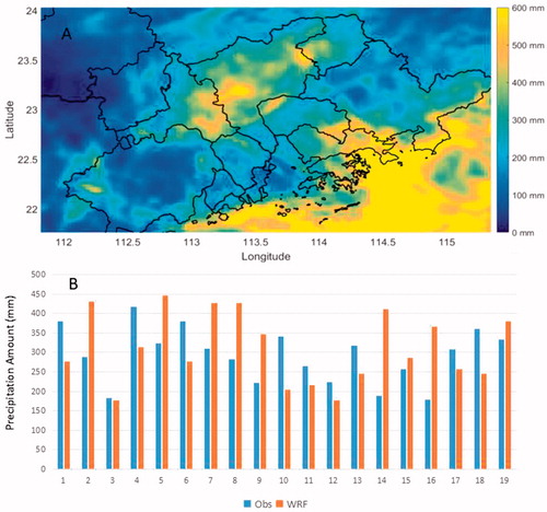
The chosen period for this sensitivity study covers 3–13 September 2010. During these 11 days, the hourly lowest temperature was 24.2 °C, and the highest temperature reached up to 32.4 °C as recorded by the Hong Kong Observatory. The effects of strong heat convection and the tropical depression brought heavy precipitation events to the PRD region during the study period. Figure 2 shows the accumulated spatial precipitation map (simulated by the WRF) and the accumulated amount (by observation and the WRF) over the study region during these 11 days. As we can see, the precipitation simulation by WRF can generally match the magnitude of the precipitation among the 19 observation stations. The total precipitation amount during these 11 days varies a lot, ranging from 183 mm to 418 mm. From the spatial map, the rainfall in some areas in Guangzhou and Hong Kong exceeded 400 mm during the study period.

Fig. 2. (A–B): Simulated geographic distribution of accumulated precipitation mapping (by WRF) in the PRD region during September 3–13, 2010 (A). The numbers on the x-axis in subfigure B represent different precipitation observation stations. The geological locations of these stations can be found in Fig. 1c, marked by red numbers.

2.4 Site and observation data

The HKUST super site (22.33 N, 114.27 E) is located on the east coast of Hong Kong in the Sai Kung area. The sampling site is surrounded by rural areas with little anthropogenic emission. The site is influenced by the southern wind during the summer and polluted northern wind from the PRD region in winter. We measured the hourly , and data using the Monitor for AeRosols and Gases in ambient Air (MARGA) instrument (ADI 2080 1S, Metrohm AG). The rain intensity is measure by TE525 rain gage (Texas Electronics) with a time resolution of 1 minute. More details can be found in Huang et al. (2014) and Griffith et al. (2015) for the super site and MARGA used in this study.

3. Results

3.1 PM_2.5 simulation sensitivity due to different BCW schemes

As discussed in Section 2, different models have different BCW schemes and hence cause discrepancies in the PM_2.5 simulation during rainy days. We incorporate different BCW schemes from other models into CAMx v6.00. In this section, we discuss the sensitivity of the PM_2.5 simulation.

The model simulation performance (including mean concentration for observation and model simulation, mean bias, mean error, normalized mean bias and normalized mean error) for PM_2.5 using different BCW schemes is shown in Table 2. The introduction of Cases A-N can be found in Section 2.1. Please note that the comparison here cannot be used to determine which BCW scheme is better, since the model performance is also influenced by other factors. This table can reveal the overall simulation difference by using various schemes over the 10 observation stations. Regarding the temporal mean bias of the PM_2.5 simulation during the study period, the results (mean) simulated by using Laakso et al. (2003) is the closest to the observation data. Some BCW schemes cause the average simulated PM_2.5 concentrations to be higher than the observation data, such as the schemes in CAMx v6.00 and Wang et al. (2014a), and some schemes underestimated the PM_2.5 concentration, such as the schemes in CMAQ, CALPUFF, and ADMS. As shown in Table 2, by using different BCW schemes, the mean error ranges from 14.3 μg m⁻³ to 17.0 μg m⁻³, the mean bias ranges from −10.5 μg m⁻³ to 4.1 μg m⁻³, the normalized mean error ranges from 0.64 to 0.77 and the normalized mean bias ranges from −0.47 to 0.20.

Table 2. Model statistical metrics using different BCW schemes.

Case	Scheme	Mean	MB	ME	NMB	NME
A	CAMx v6.00	26.5	4.1	17.0	0.20	0.77
B	CAMx v6.40	18.9	−3.5	14.9	−0.15	0.67
C	Loosmore et al. (2004)	25.3	2.9	16.9	0.15	0.76
D	AURAMS	25.2	2.8	16.4	0.14	0.74
E	EMEP	24.1	1.7	16.0	0.09	0.72
F	CMAQ	11.9	−10.5	14.9	−0.47	0.67
G	CALPUFF	16.0	−6.4	14.9	−0.28	0.67
H	ADMS	16.6	−5.8	14.6	−0.26	0.65
I	Sparmacher et al. (1993)	26.0	3.6	16.8	0.18	0.76
J	Laakso et al. (2003)	23.5	1.1	15.6	0.06	0.70
K	Wang et al. (2014c)	20.2	−2.2	14.3	−0.09	0.64
L	Baklanov and Sorensen. (2001)	16.9	−5.5	14.7	−0.24	0.66
M	Kang et al. (2015)	26.5	4.1	17.0	0.20	0.77
N	Wang et al. (2014a)	26.3	3.9	16.9	0.19	0.75
	Observations	22.4

‘Mean’ represents the mean PM_2.5 concentration over the 10 observation stations in the study period; ‘MB’ represents the mean bias; ‘ME’ represents the mean error; ‘NMB’ represents the normalized mean bias; ‘NME’ represents the normalized mean error. The lowest values for MB, ME, NMB and NME are bolded.

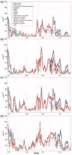
Figure 3 shows the time series difference during the study period at Tung Chung, Tai Po, Tsuen Wan, and Wanqingsha stations. Different BCW schemes do not modify the trend of the PM_2.5 simulation. After September 10th, in Tsuen Wan and Tai Po stations, almost all of the simulated peak PM_2.5 concentrations by different schemes are over 30 μg m⁻³, except the CMAQ scheme, which agrees well with the observation data. The simulation difference by various schemes reaches the highest during 9.10–9.12, because the rain intensity in this period is large, for example, the precipitation amount for most of the stations in this period is around 100 mm. Based on this comparison, different BCW schemes reveal that the PM_2.5 simulation is largely sensitive. For example, among the 10 verified stations, the mean simulated PM_2.5 concentration ranges from 11.9 μg m⁻³ (CMAQ) to 26.5 μg m⁻³ (CAMx v6.00). One should note that the simulation difference by CMAQ scheme is caused by both in-cloud rainout and below-cloud washout, since the CMAQ scheme does not separate out these two processes. Figure S1 shows the simulated PM_2.5 concentration difference between each individual scheme and the mean of the 14 BCW schemes over the 10 verified stations. As can be seen, cases F-H and L are substantially lower than the mean, while cases A, D, M, N are above the mean of the 14 cases. Cases K and J are closed to the mean of the 14 cases.

Fig. 3. Time series of PM_2.5 simulation using different BCW schemes at Tung Chung (a), Tai Po (b), Tsuen Wan (c), and Wanqingsha (d) stations.

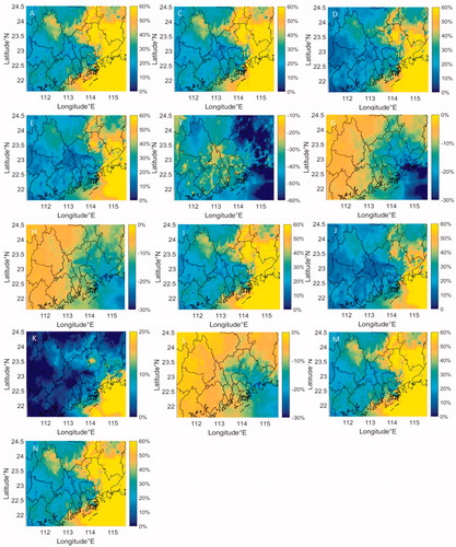
The spatial difference of the PM_2.5 simulation using different BCW schemes can be found in Fig. 4. The PM_2.5 concentrations simulated from the four BCW schemes (CMAQ, CALPUFF, ADMS, and Baklanov and Sorensen (2001)) are smaller than that simulated by the CAMx v6.40 scheme in the 3-km domain. As expected, the difference is large in the eastern part of the simulation region, where the precipitation was heavy during the simulation period. As shown in Fig. 4A, the spatial difference between CAMx v6.00 and CAMx v6.40 is large; hence, more verification is needed to understand which scheme is more suitable in this region during rainy periods.

Fig. 4. Spatial difference (compared to CAMx v6.40) of PM_2.5 simulation by using different BCW schemes (Unit: %). Letter labels on the panels refer to the simulations described in Table 2.

The average PM_2.5 concentration simulated by different BCW schemes for each individual city can be found in Table 3. The national standard for the daily average PM_2.5 concentration is 35 μg m⁻³. Hence, if we had used some BCW schemes, such as those in CAMx v6.00 and EMEP, the PM_2.5 concentrations in Guangzhou, Foshan, and Dongguan would have exceeded the standard concentration during the study period. However, if the BCW schemes from CAMx v6.40, CALPUFF, ADMS, and CMAQ had been applied, the PM_2.5 concentration in all of the cities would have reached the air quality standard. This does not mean the results would be the same if the original ADMS, CALPUFF, and CMAQ model had been used to do the simulation during the study period. The ambient PM_2.5 simulation is also determined by several other factors, such as the aerosol size bin, precursor concentration, and advection/diffusion schemes implemented in a specific model. According to Duhanyan and Roustan (2011), various BCW schemes exist for the gas-phase PM_2.5 precursors, such as SO₂ and HNO₃, which can also influence the PM_2.5 concentration. In this study, the gas-phase washout scheme is the same for all of the simulations.

Table 3. PM_2.5 average simulated concentration (μg m⁻³) by different BCW schemes for each city during the study period.

City*	A	B	C	D	E	F	G	H	I	J	K	L	M	N
HZ	20.1	12.7	19.4	18.8	17.9	6.9	10.3	10.7	19.7	18.3	13.8	11.0	20.1	20.1
GZ	40.2	30.2	38.7	38.6	36.5	20.2	26.1	26.8	39.4	37.4	31.3	27.2	40.1	40.1
FS	40.6	33.5	39.8	39.3	38.3	24.6	30.1	30.6	40.1	38.7	34.1	31.0	40.6	40.6
DG	44.3	35.1	42.9	42.8	41.1	24.5	29.5	30.6	43.6	41.6	36.0	30.9	44.2	44.2
JM	21.4	17.1	20.9	20.2	20.2	11.5	15.7	15.8	21.1	20.4	17.3	16.1	21.3	21.4
SZ	35.8	27.1	34.4	34.5	32.8	18.4	22.7	23.7	35.3	33.5	28.6	23.9	35.8	35.8
ZS	30.9	24.3	29.9	29.6	28.8	17.1	21.5	22.0	30.4	29.1	25.0	22.3	30.8	30.8
ZQ	27.2	21.4	26.8	25.9	25.8	14.5	19.7	19.9	26.9	26.0	21.9	20.3	27.2	27.2
HK	22.1	15.0	20.9	20.9	19.8	8.8	12.5	13.0	21.7	20.3	16.3	13.3	22.1	22.1
ZH	23.2	17.5	22.3	22.0	21.4	12.1	15.8	16.1	22.8	21.9	18.3	16.3	23.1	23.2

* The cities are identified in Fig. 1.

Table 2 describes the simulations A-N and Fig. 1 defines the city acronyms and shows their locations.

3.2 PM_2.5 simulation sensitivity due to different raindrop size distributions

As discussed in Section 2, the scavenging coefficient is dependent on the raindrop size distribution. In the past several decades, numerous raindrop size distribution expressions have been proposed. The raindrop size distribution comparison is based on the scheme in CAMx v6.40. Three types of size distribution are compared in this work, including exponential distribution, gamma distribution, and lognormal distribution. Twelve different raindrop size distribution parameterization schemes were implemented into CAMx model. As shown in Fig. 5, the PM_2.5 simulated concentration was the lowest by using the scheme proposed by Marshall and Palmer (1948) during the study period, while implementing Das et al. (2017) derived the highest concentration (mean of the simulation period). The difference becomes larger during the heavy rain period. For example, at Tsuen Wan site, the simulated precipitation accumulative amount from 9.10–9.12 was 108.9 mm, the average PM_2.5 concentration simulated by Das et al. (2017) was 28.6 μg m⁻³, while the concentration simulated by Marshall and Palmer (1948) was only 20.8 μg m⁻³. At Tai Po site, the average PM_2.5 simulation difference by these two methods reaches 10 μg m⁻³. Figure S2 shows the PM_2.5 concentration difference between mean of the cases A-L and each individual case. PM_2.5 simulated by cases A, B, E is lower than the mean of A-L; the concentration simulated by cases H and I are above the average. Compared to Figure S1, the variation magnitude caused by different raindrop size distribution is relatively smaller than that caused by different BCW schemes.

Fig. 5. Time series of PM_2.5 simulation using different raindrop size distribution parameterizations at Tung Chung (a), Tai Po (b), Tsuen Wan (c) and Wanqingsha (d) stations.

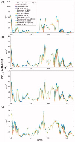
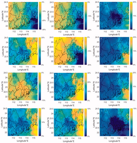
The spatial difference caused by the raindrop size distribution can be found in Fig. 6. From the spatial perspective, the PM_2.5 concentrations simulated by implementing the schemes proposed in Marshall and Palmer (1948), Ulbrich (1983), Chapon et al. (2008) and Aoki et al. (2016) (panels A, B, E, G) are lower than that simulated by CAMx v6.40, and the discrepancy can reach −30% in the eastern part of the study domain. The results simulated by the other schemes are higher than that simulated by CAMx v6.40, especially for Das et al. (2017) (panel H); the difference is more than 30% in the eastern part of the study domain. The difference caused by Harikumar et al. (2010) (panel L) is limited, and the discrepancy is smaller than 5% in the central part of the domain (Guangzhou, Foshan and Dongguan). Local field observation for the raindrop spectra is needed to determine which distribution is more suitable for this region. The simulation results may not be the same if these raindrop size distributions are implemented in other models (e.g. WRF-Chem, EMEP and so on).

Fig. 6. Spatial difference (compared to CAMx v6.40) of PM_2.5 simulation by using different raindrop size distribution parameterizations (Unit: %). Letter labels on the panels refer to the simulations described in Table 1.

3.3 Sensitivity of the source apportionment results

In addition to the PM_2.5 ambient concentration, researchers and policymakers have focused on the PM_2.5 source apportionment results; for example, the control strategy can only be made once the major sources of PM_2.5 are understood. According to Wu et al. (2013), the source region in this area can be classified into a local source (pollutant coming from the local city), a regional source (pollutant coming from other cities within the PRD region), and a super-regional source (pollutant coming from the cities outside the PRD region). When the prevalent wind direction is northern, northeastern, and northwestern, the PRD region is influenced by pollutants coming from central or northern China. Wu et al. (2013) reported that the super-regional contribution to PM_2.5 in the PRD region could reach up to 60% in December. September is the transition season in this region, in which the wind field is governed by both southern and northern directions (Lu et al., 2015).

We test how the five BCW schemes in CAMx v6.00, CAMx v6.40, EMEP, ADMS, and CALPUFF influence the PM_2.5 source apportionment results (These models are widely implemented around the world). We track three PM_2.5 compositions using the PSAT module: , , and NH₄⁺, which are the three most important anthropogenic particulate compositions in the atmosphere. Substantial parts of these three components are generated via secondary formation and enter this region by long-range transport (Wu et al., 2013). Hence, the BCW process may decrease the concentration of ambient PM_2.5 in the transport process and as a result influence the source apportionment results.

Table 4 shows the source contribution (local, regional and super-regional) to the sum of the three PM_2.5 components using the BCW schemes in three regional scale models (CAMx v6.00, CAMx v6.40, and EMEP). The difference between CAMx v6.40 and CAMx 6.00 is relatively large in some of the cities within this region (around 10% of super-regional contribution in some cities) because the washout efficiency has been increased for the updated version of CAMx. For example, when using the CAMx v6.40 BCW scheme, the local, regional, and super-regional contributions are 23.0%, 19.6%, and 57.4% in Huizhou City, respectively; when the CAMx v6.00 BCW scheme is used, the three contributions are 17.3%, 16.4%, and 66.4%, respectively. The discrepancy between these two schemes on the super-regional contribution reaches 9%. The source apportionment differences are also large in Hong Kong. With the updated BCW scheme in CAMx v6.40, the differences in regional and super-regional contribution are substantial which reach 8.6% and 11.9%, respectively. The source contribution differences in Dongguan and Shenzhen are also relatively large. The discrepancy is small in Zhaoqing, where the super-regional difference is only 3%. The source apportionment results simulated using the EMEP BCW scheme are similar to the results using CAMx v6.00. The difference in the source apportionment result is relatively large (∼10% in the super-regional contribution) in four of 10 cities using different BCW schemes. The source apportionment results simulated using the BCW schemes of CALPUFF and ADMS can be found in Table S2. In general, the difference between these two models is relatively small, and the results are similar to those of the CAMx v6.40 BCW scheme. Hence, it is necessary to discuss the sensitivity caused by the BCW schemes in the transition season if policy-related source apportionment research is carried out in this region in the future. Please note that the source apportionment results may be different with these BCW schemes by using other source apportionment method (e.g. CMAQ-ISAM).

Table 4. Source contribution (in %) to the sum of three PM_2.5 components (, and ).

	CAMx v6.40			CAMx v6.00			EMEP
City	Local	Regional	S-regional	Local	Regional	S-regional	Local	Regional	S-regional
HZ	23.0	19.6	57.4	17.3	16.4	66.4	18.4	16.7	64.9
GZ	30.2	17.8	52.0	26.7	16.0	57.4	27.4	16.3	56.3
FS	29.3	19.1	51.5	26.3	17.1	56.6	26.9	17.5	55.6
DG	23.9	33.0	43.1	18.6	28.8	52.6	19.8	29.8	50.4
JM	21.2	8.6	70.2	19.5	7.7	72.8	19.8	7.8	72.3
SZ	34.5	26.3	39.2	26.9	22.8	50.3	28.7	23.5	47.8
ZS	20.1	25.8	54.1	18.2	22.0	59.8	18.7	22.8	58.6
ZQ	18.9	15.4	65.7	17.6	13.7	68.7	17.8	13.8	68.3
HK	18.4	33.0	48.6	15.1	24.4	60.5	16.0	26.2	57.8
ZH	16.3	21.3	62.4	14.3	17.2	68.5	14.9	18.2	67.0

Figure 1 defines the city acronyms and shows their locations.

3.4 Field observation data analysis

A discrepancy (10¹ to 10² order of magnitude) exists between the BCW coefficients calculated using the theoretical method (e.g., CAMx v6.00) and the field observation (e.g., Laakso et al., 2003; Wang et al., 2014c). This may due to many factors, such as turbulence mixing effect, raindrop evaporation, and rear capturing by raindrop (Lemaitre et al., 2017). Maria and Russell (2005) pointed out that this could be due to the aerosol composition effect—the solubility of the inorganic (e.g., sulphate) and hydrophobic (e.g., organic matter) aerosol species in rainwater is not the same. In this study, we integrate the , , and data measured by MARGA together with precipitation data measured at the HKUST super site into Equation (3)(3) $$\lambda (d_a)=-\frac{1}{t_1-t_0}\ln \left[\frac{c_1(d_a)}{c_0(d_a)}\right]$$(3) to calculate the BCW coefficient of the inorganic species. The period chosen for this investigation is the summer season, during June 2016 to August 2016, when the precipitation event is frequent in this region. We further select the period when the wind speed is less than 3 m s⁻¹, the RH difference (before and after the rain event) is less than 10%, the rain intensity is larger than 2 mm h⁻¹, and the rain event duration is longer than 10 minutes for analysis (Laakso et al., 2003; Maria and Russell, 2005). Under such conditions, changes in the aerosol concentration should be due to rain scavenging instead of other factors (Laakso et al., 2003). Still, some factors influencing the change of PM_2.5 concentration cannot be ruled out, such as the vertical mixing.

Table 5 shows the BCW coefficients for , , and during summer 2016. The median values of the BCW coefficient for , , and are 1.4 × 10⁻⁴, 3.2 × 10⁻⁴, and 2.0 × 10⁻⁴s⁻¹, respectively. These values are on the same magnitude as the average value from Claassen and Halm (1995), but are slightly larger than the coefficients reported by Maria and Russell (2005) (: 7.8 × 10⁻⁵s⁻¹; : 6.7 × 10⁻⁵s⁻¹). One possible reason for this discrepancy is that the sampling time resolution in Maria and Russell (2005) is coarser than that in this study and that (t1-t0) in Equation (3)(3) $$\lambda (d_a)=-\frac{1}{t_1-t_0}\ln \left[\frac{c_1(d_a)}{c_0(d_a)}\right]$$(3) may include the period that did not have rain in their work. The calculated BCW coefficients in this study are also larger than those calculated using the theoretical method (the CAMx model), which is on the magnitude of 10⁻⁷ to 10⁻⁶.

Table 5. The BCW coefficients calculated by field observation data at the HKUST super-site.*

Time (DD_HHMM)	(s^−1)	(s^−1)	(s^−1)	Precip (mm)	Duration (min)
6.06_6:00-7:59	1.9 × 10^−4	3.4 × 10^−4	8.7 × 10^−5	16.8	21
6.08_1:00-5:59	4.5 × 10^−4	3.2 × 10^−4	2.7 × 10^−4	35.0	72
6.10_18:00-18:59	3.6 × 10^−4	3.2 × 10^−4	2.5 × 10^−4	10.9	26
6.10_21:00-21:59	5.9 × 10^−4	5.6 × 10^−4	4.0 × 10^−4	5.6	15
6.11_11:00-12:59	−5.1 × 10^−5	2.4 × 10^−4	1.2 × 10^−4	12.4	43
6.12_7:00-8:59	−1.1 × 10^−4	1.9 × 10^−4	5.1 × 10^−5	10.7	32
6.12_10:00-10:59	2.4 × 10^−4	−1.7 × 10^−4	3.9 × 10^−4	4.3	15
6.17_4:00-4:59	2.9 × 10^−4	7.7 × 10^−4	1.4 × 10^−4	5.8	13
6.17_7:00-7:59	2.0 × 10^−4	2.8 × 10^−4	1.7 × 10^−4	8.4	17
7.09_22:00-22:59	−3.0 × 10^−5	4.7 × 10^−4	−9.5 × 10^−5	10.4	16
7.11_3:00-3:59	2.7 × 10^−4	3.9 × 10^−4	1.9 × 10^−4	4.3	12
7.11_6:00-6:59	6.9 × 10^−5	2.2 × 10^−4	9.0 × 10^−5	11.9	21
7.13_7:00-7:59	2.4 × 10^−5	8.3 × 10^−5	2.2 × 10^−5	15.5	41
7.14_12:00-12:59	1.6 × 10^−4	2.7 × 10^−4	2.8 × 10^−5	4.1	13
8.10_7:00-7:59	2.7 × 10^−4	5.0 × 10^−4	3.3 × 10^−4	39.6	60
8.11_9:00-11:59	7.1 × 10^−5	1.5 × 10^−4	4.7 × 10^−5	14.2	45
8.28_1:00-2:59	6.4 × 10^−4	3.4 × 10^−4	8.8 × 10^−4	14.5	35
Median	2.0 × 10^−4	3.2 × 10^−4	1.4 × 10^−4	–	–

* The HKUST super-site is in Clear Water Bay, Kowloon, Hong Kong.

The calculated BCW coefficients are implemented into the CAMx model. Because / and / are generally mixed together in the aerosol phase, the average value of the median BCW coefficients for these three species are implemented into the CAMx model (2.2 × 10⁻⁴). There are no organic matter data at the HKUST super site; the value reported by Maria and Russell (2005) (2.2 × 10⁻⁵) is used in this simulation. After the update, the PM_2.5 simulated mean value, mean bias, mean error, normalized mean bias, and normalized mean error are 22.9 μg m⁻³ (mean observation, 22.4 μg m⁻³), 0.5 μg m⁻³, 14.2 μg m⁻³, 1.9%, and 63.4%, respectively (3–13 September). The simulation performance improved (e.g. the mean bias drops down from over 3 μg m⁻³ to 0.5 μg m⁻³) in the cases simulated with CAMx v6.00 and CAMx v6.40 (Table 2), which implies that consideration of the solubility difference caused by the aerosol species in the BCW coefficient calculation may help to improve aerosol simulation during the rainy seasons in 3-D CTMs. However, the simulation result is also influenced by the in-cloud rainout process and uncertainty exists for the BCW coefficient derived from this study – only 17 cases were used to calculate the species dependent BCW coefficient. In the future, a longer period (e.g. a year) of BCW coefficient study dependent on aerosol species is highly recommended.

4. Discussion

Based on the results presented in Section 3, different numerical BCW coefficient parameterizations can cause large differences in the ambient PM_2.5 simulation during heavy rainy periods. For example, the difference between the results simulated by CMAQ and CAMx v6.00 washout schemes exceeds 50 μg m⁻³ on September 10^th. In this study, the PM_2.5 simulation by the BCW scheme from Laakso et al. (2003) is relatively closer (mean of the simulation period) to the observation data than that of other schemes. But we cannot judge which scheme is the ‘best’ in this study due to three reasons: (1) relative short simulation period, (2) the model performance is influenced by many factors, such as emission inventory, in-cloud rainout and the other chemical and physical parameterization schemes and (3) the precipitation fraction issue – within 9 km², the events of no rain, drizzle and heavy rain can take place at the same time. The simulation result by Wang et al. (2014a) is similar to the one by CAMx model. However, one should note that the method proposed by Wang et al. (2014a) is more flexible for different model frameworks and it does not require the input of the raindrop parameters, such as raindrop terminal velocity and raindrop size distribution, which can help to decrease the computational burden during the simulation. For other study, Gong et al. (2011) also compared the PM_2.5 simulation caused by two different BCW schemes and they found that in some regions the difference could reach 10%. The difference is dependent on many factors, such as the individual scheme, pollutant concentration and precipitation intensity.

The sensitivity of the PM_2.5 concentration attributed to the BCW scheme was found to influence the source apportionment results. Such a discrepancy may mislead scientists or policymakers when trying to formulate emission control policies for local governments. Our results indicate that the difference caused by the BCW coefficients can be propagated to the PM_2.5 simulation and source apportionment calculation during the rainy season and lead to large differences. For instance, the super-regional difference (source apportionment results) in Hong Kong between CAMx v6.00 and CAMx v6.40 BCW schemes exceeds 10%.

Some of the raindrop parameterizations are based on the data collected from the single campaign. For example, the raindrop size distribution developed by De Wolf (2001) was based on data collected by Marshall and Palmer (1948). Related raindrop parameterizations may only be effective or fit the data in those specific campaigns and regions. This is why there have been so many different raindrop parameterizations since the 1940s. Marshall and Palmer (1948) collected the data in Canada, which does not have the subtropical climate of the PRD region. Some studies have developed raindrop parameterizations that are dependent on the type of rain, such as hurricanes, thunderstorms, and drizzle. Raindrop characteristics differ across these rain types; however, it is difficult for 3-D CTMs to characterize the rain type and choose specific BCW parameterizations for the simulation. In this study, the PM_2.5 simulation difference attributed to various raindrop size distributions is relatively large during the heavy rain period. One should also note that some of the aerosol schemes in CTMs have only two (CF scheme—CAMx) or three (CMAQ) size bins. Hence, the BCW coefficient parameterization should be based on long-term experimental data and fit the aerosol size bin used in the specific CTMs or based on the schemes by using statistical fitting, such as the ones proposed by Laakso et al. (2003) and Wang et al. (2014a).

We find a large PM_2.5 simulation difference between the schemes derived by field measurement (Wang et al., 2014c) and theoretical calculation (CAMx v6.00), the difference of the simulated mean value reaches 6.3 μg m⁻³. Other studies have also found a large discrepancy between theoretically calculated and field measured BCW coefficients (Davenport and Peter, 1978; Chate and Pranesha, 2004; Wang et al., 2014a). Wang et al. (2014a) reported that the theoretical calculated BCW coefficient (e.g., that used by CAMx v6.00) was an order of magnitude smaller than that derived from a 6-year field campaign (1-mm h⁻¹ precipitation rate and 1-μm particle diameter) (Laakso et al., 2003). The hygroscopic property and solubility for different aerosol components are not the same. Maria and Russell (2005) found that significant variations of BCW coefficients were related to aerosol composition. Other factors include turbulent vertical mixing, raindrop rear capturing and so on. As such, based on available observation data, we further investigate the BCW coefficients for , and using the MARGA data at the HKUST super site. The observation-based coefficients are larger (10-10²) than those calculated by the theoretical method (Brownian movement, impaction and interception) implemented in the CAMx model. This implies that something may be missing in the traditional theoretical method and that more studies are needed in this area. However, uncertainty exists for observation-based coefficient because other physical processes (e.g. turbulent vertical mixing) occurs at the same time.

Furthermore, as discussed in Gong et al. (2011), two other aspects are needed for further study on BCW process in the future (1) the removal of precursor gas, since the BCW washing for gas is more important than its in-cloud rainout; (2) the precipitation evaporation, which was only considered in few model and hence more works are needed on this mechanism analysis. In-cloud rainout is another process that should influence the amounts of PM_2.5 concentration and wet deposition in the CTM simulation. The in-cloud rainout process is also modelled differently in different CTMs. For example, in the CAMx model, the in-cloud rainout coefficient is set to be a constant (0.9), whereas in CMAQ this process is a function of the water vapour mixing ratio and is calculated using Equations (8)(8) $$\alpha =\frac{1}{{\tau }_{washout}}$$(8) and (9)(9) $${\tau }_{washout}=\frac{{\overline{W}}_T\Delta z}{{\rho }_w{P}_{}}$$(9) . PM_2.5 is formed from gas-phase precursors, and some of the soluble precursors can be influenced by the precipitation, such as SO₂ and HNO₃. According to Gong et al. (2011), the gas-phase precursors have several BCW schemes. Therefore, in the future, it will be necessary to examine how these processes influence the PM_2.5 simulation and source apportionment results in the 3 D CTM.

5. Conclusions

This study analyses the sensitivity of PM_2.5 simulation and source apportionment results due to different BCW schemes. BCW schemes from different 3 D CTMs (e.g., CMAQ, CAMx, EMEP, and CALPUFF) as well as different raindrop size distributions are modified into the CAMx v6.00 model. The simulation difference caused by different BCW schemes during the heavy rain periods can reach up to 50 μgm⁻³. It is necessary to further evaluate the uncertainty of PM_2.5 simulation due to BCW scheme for a longer period during the rainy seasons in different region. In addition to the PRD region, some other regions in China, such as the Yangtze River Delta region, have substantial precipitation amounts during the transition season. Therefore, BCW sensitivity studies should be performed during the rainy seasons in those regions. A difference in BCW coefficients exists between laboratory experiments and field observations, which is possibly due to the composition effect. More BCW coefficient study based on aerosol composition is highly needed. Lastly, during the rainy season, the wet removal of precursor gas of PM_2.5 can also play a role in the surface PM_2.5 concentration. This process is not analyzed in this study and it is recommended to be included in the future BCW study.

Supplemental data

Supplemental data for this article can be accessed here: https://doi.org/10.1080/16000889.2018.1476435.

Acknowledgements

We appreciate the assistance of the Hong Kong Observatory (HKO), which provided the meteorological data.

Disclosure statement

No potential conflict of interest was reported by the authors.

Funding

This work was supported by NSFC Grant 41575106 and the RGC Grant 16300715.

References

- Abel, S. J. and Shipway, B. J. 2007. A comparison of cloud‐resolving model simulations of trade wind cumulus with aircraft observations taken during RICO. Qjr. Meteorol. Soc. 133, 781–794. DOI:10.1002/qj.55.
- Aikawa, M., Kajino, M., Hiraki, T. and Mukai, H. 2014. The contribution of site to washout and rainout: Precipitation chemistry based on sample analysis from 0.5 mm precipitation increments and numerical simulation. Atmos. Environ. 95, 165–174. DOI:10.1016/j.atmosenv.2014.06.015.
- Aoki, M., Iwai, H., Nakagawa, K., Ishii, S. and Mizutani, K. 2016. Measurements of rainfall velocity and raindrop size distribution using coherent Doppler lidar. J. Atmos. Ocean Tech. 33, 1949–1966. DOI: 10.1175/JTECH-D-15-0111.1
- Appel, K. W., Foley, K. M., Bash, J. O., Pinder, R. W., Dennis, R. L. and co-authors. 2011. A multi-resolution assessment of the Community Multiscale Air Quality (CMAQ) model v4. 7 wet deposition estimates for 2002–2006. Geosci. Model Dev. 4, 357–371. DOI:10.5194/gmd-4-357-2011.
- Atlas, D. 1953. Optical extinction by rainfall. J. Meteor. 10, 486–488. DOI:10.1175/1520-0469(1953)010<0486:OEBR>2.0.CO;2.
- Atlas, D., Srivastava, R. C. and Sekhon, R. S. 1973. Doppler radar characteristics of precipitation at vertical incidence. Rev. Geophys. 11, 1–35.
- Atlas, D. and Ulbrich, C. W. 1977. Path-and area-integrated rainfall measurement by microwave attenuation in the 1–3 cm band. J. Appl. Meteor. 16, 1322–1331. DOI:10.1175/1520-0450(1977)016<1322:PAAIRM>2.0.CO;2.
- Bae, S. Y., Park, R. J., Kim, Y. P. and Woo, J. H. 2012. Effects of below-cloud scavenging on the regional aerosol budget in East Asia. Atmos. Environ. 58, 14–22. DOI:10.1016/j.atmosenv.2011.08.065.
- Baklanov, A. and Sørensen, J. H. 2001. Parameterisation of radionuclide deposition in atmospheric long-range transport modelling. Phys. Chem. Earth. Part B: Hydrology, Oceans and Atmosphere 26, 787–799. DOI:10.1016/S1464-1909(01)00087-9.
- Best, A. C. 1950. Empirical formulae for the terminal velocity of water drops falling through the atmosphere. Qj. Royal Met. Soc. 76, 302–311. DOI:10.1002/qj.49707632905.
- Best, A. C. 1950. The size distribution of raindrops. Qj. Royal Met. Soc. 76, 16–36. DOI:10.1002/qj.49707632704.
- Blanchard, D. C. 1953. Raindrop size-distribution in Hawaiian rains. J. Meteor. 10, 457–473. DOI:10.1175/1520-0469(1953)010<0457:RSDIHR>2.0.CO;2.
- Brandes, E. A., Zhang, G. and Vivekanandan, J. 2002. Experiments in rainfall estimation with a polarimetric radar in a subtropical environment. J. Appl. Meteor. 41, 674–685. DOI:10.1175/1520-0450(2002)041<0674:EIREWA>2.0.CO;2.
- Campos, E. F., Zawadzki, I., Petitdidier, M. and Fernandez, W. 2006. Measurement of raindrop size distributions in tropical rain at Costa Rica. J Hydrol. 328, 98–109. DOI:10.1016/j.jhydrol.2005.11.047.
- Cerro, C., Codina, B., Bech, J. and Lorente, J. 1997. Modeling raindrop size distribution and Z (R) relations in the Western Mediterranean area. J. Appl. Meteor. 36, 1470–1479. DOI:10.1175/1520-0450(1997)036<1470:MRSDAZ>2.0.CO;2.
- Chapon, B., Delrieu, G., Gosset, M. and Boudevillain, B. 2008. Variability of rain drop size distribution and its effect on the Z–R relationship: A case study for intense Mediterranean rainfall. Atmos. Res. 87, 52–65. DOI:10.1016/j.atmosres.2007.07.003
- Chate, D. M. and Pranesha, T. S. 2004. Field studies of scavenging of aerosols by rain events. J of Aerosol. Sci. 35, 695–706. DOI:10.1016/j.jaerosci.2003.09.007.
- Chatterjee, A., Jayaraman, A., Rao, T. N. and Raha, S. 2010. In-cloud and below-cloud scavenging of aerosol ionic species over a tropical rural atmosphere in India. J. Atmos. Chem. 66, 27–40. DOI:10.1007/s10874-011-9190-5.
- Chen, F. and Dudhia, J. 2001. Coupling an advanced land surface–hydrology model with the Penn State–NCAR MM5 modeling system. Part I: Model implementation and sensitivity. Monthly Weather Rev. 129, 569–565. DOI:10.1175/1520-0493(2001)129<0569:CAALSH>2.0.CO;2.
- Chen, B., Hu, Z., Liu, L. and Zhang, G. 2017. Raindrop Size Distribution Measurements at 4,500 m on the Tibetan Plateau During TIPEX-III. J. Geophys. Res, 122. DOI: 10.1002/2017JD027233
- Chen, B., Yang, J. and Pu, J. 2013. Statistical characteristics of raindrop size distribution in the Meiyu season observed in Eastern China. J. Meteorol. Soc. Japan. 91, 215–227. 85. DOI:10.2151/jmsj.2013-208.
- Coutinho, M. A. and Tomás, P. P. 1995. Characterization of raindrop size distributions at the Vale Formoso Experimental Erosion Center. Catena. 25, 187–197. DOI:10.1016/0341-8162(95)00009-H.
- Das, S. K., Konwar, M., Chakravarty, K. and Deshpande, S. M. 2017. Raindrop size distribution of different cloud types over the Western Ghats using simultaneous measurements from Micro-Rain Radar and disdrometer. Atmos. Res. 186, 72–82. DOI:10.1016/j.atmosres.2016.11.003
- Davenport, H. M. and Peters, L. K. 1978. Field studies of atmospheric particulate concentration changes during precipitation. Atmos. Environ. (1967) 12, 997–1008. DOI:10.1016/0004-6981(78)90344-X.
- de Wolf, D. A. 2001. On the Laws-Parsons distribution of raindrop sizes. Radio Sci. 36, 639–642.
- Dudhia, J. 1989. Numerical study of convection observed during the winter monsoon experiment using a mesoscale two-dimensional model. J. Atmos. Sci. 46, 3077–3107. DOI:10.1175/1520-0469(1989)046<3077:NSOCOD>2.0.CO;2.
- Dudhia, J., Hong, S. Y. and Lim, K. S. 2008. A new method for representing mixed-phase particle fall speeds in bulk microphysics parameterizations. JMSJ. 86A, 33–44. DOI:10.2151/jmsj.86A.33.
- Duhanyan, N. and Roustan, Y. 2011. Below-cloud scavenging by rain of atmospheric gases and particulates. Atmos Environ. 45, 7201–7217. DOI:10.1016/j.atmosenv.2011.09.002.
- Feingold, G. and Levin, Z. 1986. The lognormal fit to raindrop spectra from frontal convective clouds in Israel. J. Climate Appl. Meteor. 25, 1346–1363. DOI:10.1175/1520-0450(1986)025<1346:TLFTRS>2.0.CO;2.
- Gong, W., Stroud, C. and Zhang, L. 2011. Cloud processing of gases and aerosols in air quality modeling. Atmosphere. 2, 567–616. DOI:10.3390/atmos2040567.
- Grell, G. A. and Dévényi, D. 2002. A generalized approach to parameterizing convection combining ensemble and data assimilation techniques. Geophys. Res. Lett. 29, 38-1.
- Griffith, S. M., Huang, X. H., Louie, P. K. K. and Yu, J. Z. 2015. Characterizing the thermodynamic and chemical composition factors controlling PM 2.5 nitrate: Insights gained from two years of online measurements in Hong Kong. Atmos Environ. 122, 864–875. DOI:10.1016/j.atmosenv.2015.02.009.
- Guenther, A., Karl, T., Harley, P., Wiedinmyer, C., Palmer, P. I. and co-authors. 2006. Estimates of global terrestrial isoprene emissions using MEGAN (Model of Emissions of Gases and Aerosols from Nature). Atmos. Chem. Phys. 6, 3181–3210. DOI:10.5194/acp-6-3181-2006.
- Han, Z., Ueda, H. and Sakurai, T. 2006. Model study on acidifying wet deposition in East Asia during wintertime. Atmos. Environ. 40, 2360–2373. DOI:10.1016/j.atmosenv.2005.12.017.
- Harikumar, R., Sampath, S. and Kumar, V. S. 2010. Variation of rain drop size distribution with rain rate at a few coastal and high altitude stations in southern peninsular India. Adv. Space Res. 45, 576–586. DOI: 10.1016/j.asr.2009.09.018
- Huang, X. H., Bian, Q., Ng, W. M., Louie, P. K. and Yu, J. Z. 2014. Characterization of PM2. 5 major components and source investigation in suburban Hong Kong: a one year monitoring study. Aerosol Air Qual. Res. 14, 237–250.
- Hong, S. Y., Noh, Y. and Dudhia, J. 2006. A new vertical diffusion package with an explicit treatment of entrainment processes. Mon. Wea. Rev. 134, 2318–2341. DOI:10.1175/MWR3199.1.
- Kang, Y., Hua, F., Zhong, K. and Zhu, H. 2015. A new analysis of fine aerosol capture by raindrops at terminal velocities. J. Aero. Sci. 89, 31–42. DOI:10.1016/j.jaerosci.2015.06.007.
- Kessler, E. 1969. On the distribution and continuity of water substance in atmospheric circulations. In On the Distribution and Continuity of Water Substance in Atmospheric Circulations (pp. 1–84). American meteorological society.
- Kwok, R. H. F., Napelenok, S. L. and Baker, K. R. 2013. Implementation and evaluation of PM 2.5 source contribution analysis in a photochemical model. Atmos. Environ. 80, 398–407. DOI:10.1016/j.atmosenv.2013.08.017.
- Laws, J. O. and Parsons, D. A. 1943. The relation of raindrop‐size to intensity. Trans. Agu. 24, 452–460. DOI:10.1029/TR024i002p00452.
- Laakso, L., Grönholm, T., Rannik, Ü., Kosmale, M., Fiedler, V. and co-authors. 2003. Ultrafine particle scavenging coefficients calculated from 6 years field measurements. Atmos. Environ. 37, 3605–3613. DOI:10.1016/S1352-2310(03)00326-1.
- Lemaitre, P., Querel, A., Monier, M., Menard, T., Porcheron, E. and co-authors. 2017. Experimental evidence of the rear capture of aerosol particles by raindrops. Atmos. Chem. Phys. 17, 4159–4176. DOI:10.5194/acp-17-4159-2017.
- Li, Y., Lau, A. K. H., Fung, J. C. H., Zheng, J. Y., Zhong, L. J. and co-authors. 2012. Ozone source apportionment (OSAT) to differentiate local regional and super‐regional source contributions in the Pearl River Delta region, China. J. Geophys. Res. 117, n/a.
- Liu, J. Y. and Orville, H. D. 1969. Numerical modeling of precipitation and cloud shadow effects on mountain-induced cumuli. J. Atmos. Sci. 26, 1283–1298. DOI:10.1175/1520-0469(1969)026<1283:NMOPAC>2.0.CO;2.
- Loosmore, G. A. and Cederwall, R. T. 2004. Precipitation scavenging of atmospheric aerosols for emergency response applications: testing an updated model with new real-time data. Atmos. Environ. 38, 993–1003. DOI:10.1016/j.atmosenv.2003.10.055.
- Lu, X., Fung, J. C. H. and Wu, D. 2015. Modeling wet deposition of acid substances over the PRD region in China. Atmos. Environ. 122, 819–828. DOI:10.1016/j.atmosenv.2015.09.035.
- Lu, X., Yao, T., Li, Y., Fung, J. C. H. and Lau, A. K. H. 2016. Source apportionment and health effect of NO x over the Pearl River Delta region in southern China. Environ. Pollut. 212, 135–146. DOI:10.1016/j.envpol.2016.01.056.
- Marshall, J. S. and Palmer, W. M. K. 1948. The distribution of raindrops with size. J. Meteor. 5, 165–166. DOI:10.1175/1520-0469(1948)005<0165:TDORWS>2.0.CO;2.
- Maria, S. F. and Russell, L. M. 2005. Organic and inorganic aerosol below-cloud scavenging by suburban New Jersey precipitation. Environ. Sci. Technol. 39, 4793–4800. DOI:10.1021/es0491679.
- Mlawer, E. J., Taubman, S. J., Brown, P. D., Iacono, M. J. and Clough, S. A. 1997. Radiative transfer for inhomogeneous atmospheres: RRTM, a validated correlated‐k model for the longwave. J. Geophys. Res. 102, 16663–16682.
- Myhre, G., Myhre, C. E. L., Samset, B. H. and Storelvmo, T. 2013. Aerosols and their relation to global climate and climate sensitivity. Nature Educ. Knowledge. 4, 7.
- Nenes, A., Pandis, S. N. and Pilinis, C. 1998. ISORROPIA: A new thermodynamic equilibrium model for multiphase multicomponent inorganic aerosols. Aqua. Geochem. 4, 123–152. DOI:10.1023/A:1009604003981.
- Roselle, S. J. and Binkowski, F. S. 1999. Cloud dynamics and chemistry, chap. 11. In: Science Algorithms of the EPA Models-3 Community Multiscale Air Quality [CMAQ] Modeling System (eds. D. W. Byun and J. S. Ching), EPA/600/R-99/030. U.S. Environ. Protect. Agency, Washington, D. C., pp. 11-1–11-8.
- Rasch, P. J., Feichter, J., Law, K., Mahowald, N., Penner, J. and co-authors. 2000. A comparison of scavenging and deposition processes in global models: results from the WCRP Cambridge Workshop of 1995. Tellus B. 52, 1025–1056. DOI:10.3402/tellusb.v52i4.17091.
- Scire, J. S., Strimaitis, D. G. and Yamartino, R. J. 2000. A User’s Guide for the CALPUFF Dispersion Model (version 5). Earth Tech, Inc., Concord, MA.
- Sekhon, R. S. and Srivastava, R. C. 1971. Doppler radar observations of drop-size distributions in a thunderstorm. J. Atmos. Sci. 28, 983–994. DOI:10.1175/1520-0469(1971)028<0983:DROODS>2.0.CO;2.
- Seinfeld, J. H. and Pandis, S. N. 2006. : Atmospheric Chemistry and Physics: From Air Pollution to Climate Change. Wiley and Sons, New Jersey.
- Simpson, D., Benedictow, A., Berge, H., Bergström, R., Emberson, L. D. and co-authors. 2012. The EMEP MSC-W chemical transport model–technical description. Atmos. Chem. Phys. 12, 7825–7865. DOI:10.5194/acp-12-7825-2012.
- Slinn, W. 1983. Precipitation Scavenging, in Atmospheric Sciences and Power Production 1979 (Chap.11). Division of Biomedical Environment Research, U.S. Department of Energy, Washington, D.C.
- Sparmacher, H., Fülber, K. and Bonka, H. 1993. Below-cloud scavenging of aerosol particles: Particle-bound radionuclides—Experimental. Atmos. Environ.. Part A. Gen. Top. 27, 605–618. DOI:10.1016/0960-1686(93)90218-N.
- Timothy, K. I., Ong, J. T. and Choo, E. B. 2002. Raindrop size distribution using method of moments for terrestrial and satellite communication applications in Singapore. IEEE Trans. Antennas Propag. 50, 1420–1424. DOI: 10.1109/TAP.2002.802091
- Ulbrich, C. W. 1983. Natural variations in the analytical form of the raindrop size distribution. J. Climate Appl. Meteor. 22, 1764–1775. DOI:10.1175/1520-0450(1983)022 < 1764:NVITAF >2.0.CO;2.
- Uplinger, W. G. 1981. A new formula for raindrop terminal velocity. In Conference on Radar Meteorology, 20 th, Boston, MA (pp. 389–391).
- Wang, X., Zhang, L. and Moran, M. D. 2010. Uncertainty assessment of current size-resolved parameterizations for below-cloud particle scavenging by rain. Atmos Chem Phys. 10, 5685–5705. DOI:10.5194/acp-10-5685-2010.
- Wang, X., Zhang, L. and Moran, M. D. 2014a. Development of a new semi-empirical parameterization for below-cloud scavenging of size-resolved aerosol particles by both rain and snow. Geosci. Model Dev. 7, 799–819. DOI:10.5194/gmd-7-799-2014.
- Wang, Y., Li, L., Chen, C., Huang, C., Huang, H. and co-authors. 2014b. Source apportionment of fine particulate matter during autumn haze episodes in Shanghai, China. J. Geophys. Res. Atmos. 119, 1903–1914. DOI:10.1002/2013JD019630.
- Wang, Y., Zhu, B., Kang, H., Gao, J., Jiang, Q. and co-authors. 2014c. Theoretical and observational study on below-cloud rain scavenging of aerosol particles. J. Univ. Chin. Acad. Sci.. 31, 306–313. In Chinese).
- Wang, P. K. and Pruppacher, H. R. 1977. Acceleration to terminal velocity of cloud and raindrops. J. Appl. Meteor. 16, 275–280. DOI:10.1175/1520-0450(1977)016<0275:ATTVOC>2.0.CO;2.
- Wu, D., Fung, J. C. H., Yao, T. and Lau, A. K. H. 2013. A study of control policy in the Pearl River Delta region by using the particulate matter source apportionment method. Atmos. Environ. 76, 147–161. DOI: 10.1016/j.atmosenv.2012.11.069
- Zikova, N. and Zdimal, V. 2016. Precipitation scavenging of aerosol particles at a rural site in the Czech Republic. Tellus B: Chem. Phys. Meteorol. 68, 27343. DOI:10.3402/tellusb.v68.27343.
- Zhang, L. and Vet, R. 2006. A review of current knowledge concerning size-dependent aerosol removal. China Particuology. 4, 272–282. DOI:10.1016/S1672-2515(07)60276-0.
- Zhang, Q., Streets, D. G., Carmichael, G. R., He, K. B., Huo, H. and co-authors. 2009. Asian emissions in 2006 for the NASA INTEX-B mission. Atmos. Chem. Phys. 9, 5131–5153. DOI:10.5194/acp-9-5131-2009.
- Zheng, J., Zhang, L., Che, W., Zheng, Z. and Yin, S. 2009. A highly resolved temporal and spatial air pollutant emission inventory for the Pearl River Delta region, China and its uncertainty assessment. Atmos. Environ. 43, 5112–5122. DOI:10.1016/j.atmosenv.2009.04.060.
- Zhao, H. and Zheng, C. 2006. Monte Carlo solution of wet removal of aerosols by precipitation. Atmos. Environ. 40, 1510–1525. DOI:10.1016/j.atmosenv.2005.10.043.
- Zhang, L., Wang, X., Moran, M. D. and Feng, J. 2013. Review and uncertainty assessment of size-resolved scavenging coefficient formulations for below-cloud snow scavenging of atmospheric aerosols. Atmos. Chem. Phys. 13, 10005–10025. DOI:10.5194/acp-13-10005-2013.