Estimates of methane emissions from the Southern Ocean from quasi-continuous underway measurements of the partial pressure of methane in surface seawater during the 2012/13 austral summer

Abstract

We used a new underway measurement system to investigate the partial pressure of methane (CH₄) in surface seawater and overlying air in the Southern Ocean from late November 2012 to mid-February 2013. The underway system consisted of a cavity ring-down spectroscopy analyser and a shower-head type equilibrator. The monthly mean atmospheric CH₄ mixing ratios obtained agreed well (within 5 ppb) with those recorded at onshore baseline stations. CH₄ saturation ratios (SR, %), defined as CH₄ concentration in seawater divided by CH₄ concentration equilibrated with atmospheric CH₄, varied between 85 and 185%; most of the ratios we calculated indicated supersaturation, except for those from south of the Southern limit of Upper Circumpolar Deep Water. SR was higher at the lower latitudes, including coastal areas north of the Sub-Antarctic Front, but decreased gradually and monotonously between the Sub-Antarctic Front and the Upper Circumpolar Deep Water. At high latitudes south of the Polar Front, SR decreased to below 100% due to the effects of upwelling and vertical mixing. We found a strong linear correlation between SR and apparent oxygen utilisation (AOU) south of the Polar Front. Observed SR decreased with increasing AOU and reached 85% at high AOU (41 µmol kg⁻¹) and low temperature (–1.8 °C). On the basis of the linear relationship between SR and AOU, we evaluated the climatological sea–air flux of CH₄ from December to February for the entire Southern Ocean south of 50°S: Sea–air CH₄ emission was estimated to be 0.027 Tg yr⁻¹ in December, 0.04 Tg yr⁻¹ in January, and 0.019 Tg yr⁻¹ in February.

Keywords:

• dissolved CH₄ distribution
• Southern Ocean
• CRDS coupling with an equilibrator
• CH₄ emission
• oceanic fronts
• sea–air exchange

1. Introduction

Methane (CH₄) is a potent greenhouse gas that plays a major role in both tropospheric and stratospheric chemistry (Cicerone and Oremland, 1988; Crutzen and Zimmermann, 1991). There is recent evidence that the tropospheric CH₄ mixing ratio has increased dramatically over a 100-year time scale. During the last two centuries, the mixing ratio of atmospheric CH₄ has increased by 1000 ppb, reaching 1834 ppb in 2015, as a result of anthropogenic activities (Dlugokencky et al., 1994; www.esrl.noaa.gov/gmd/ccgg/trends_ch4/). Although the world’s oceans are a source of CH₄, they are thought to play only a minor role in the global CH₄ budget; oceanic emissions account for only a few percent of all natural and anthropogenic sources (Cicerone and Oremland, 1988; Conrad and Seiler, 1988; Crutzen and Zimmermann, 1991; Bange et al., 1994). Although major sources and sinks of atmospheric CH₄ have been identified, great uncertainties remain in estimations of the total earth and atmospheric budgets of CH₄ (Saunois et al., 2016).

Dissolved CH₄ in surface ocean waters tends to be supersaturated with respect to atmospheric CH₄ (Conrad and Seiler, 1988; Crutzen and Zimmermann, 1991; Bates et al., 1993; Tilbrook and Karl, 1995). Dissolved CH₄ concentrations are supersaturated throughout the equatorial and tropical regions of the Pacific Ocean (Bates et al., 1996; Yoshida et al., 2011), but both supersaturation and undersaturation are known in the extratropics (Kelley and Jeffrey, 2002) and at high latitudes (Bates et al., 1996; Yoshida et al., 2011). The main factors that control CH₄ supersaturation in tropical and extratropical regions are equatorial upwelling and seasonal variations of sea surface temperature (SST), respectively (Bates et al., 1996). In the pelagic zone, bacterial CH₄ is released from the digestive tracts of zooplankton and from sinking organic particles; CH₄ is removed from ocean waters by microbial oxidation and by the sea–air flux (Grunwald et al., 2009). In productive coastal areas, large amounts of CH₄ are produced by methanogenesis in buried sediment layers, which account in part for the high contribution of coastal areas and estuaries to the sea–air flux of CH₄ (Bange et al., 1994).

In the Arctic Ocean, massive amounts of CH₄ stored in gas hydrates and permafrost within warming shallow marine sediments have resulted in CH₄ supersaturation in the water column in areas such as the Laptev and East Siberian Seas (James et al., 2016; Thornton et al., 2016). Undersaturation of CH₄ deep in the water column in the Arctic Ocean is a result of microbial oxidation (Rehder et al., 1999) and is consistent with the maximum seawater temperature in the core of Warm Deep Water (Heeschen et al., 2004).

In the Southern Ocean, low CH₄ in surface water is a consequence of entrainment by surface water of deep water depleted in CH₄ (Yoshida et al., 2011) because of its low content of organic particles (Fischer et al., 1988), upwelling of old deep water (Rehder et al., 1999; Heeschen et al., 2004), or both.

The CH₄ is produced by microbial methanogenesis in anaerobic environments and by bacteria in organic particles or in the gut of zooplankton (Karl and Tilbrook, 1994). Methanogens have been shown to be zooplankton-species-specific (de Angelis and Lee, 1994), which contributes to the lack of a consistent correlation between CH₄ concentrations in seawater and commonly measured biological parameters. Burke et al. (1983) reported weak correlations between CH₄ concentrations and particulate and biological parameters in the eastern tropical North Pacific and that the CH₄ distribution there was largely controlled by physical oceanographic processes.

The Southern Ocean is one of the most biologically productive oceanic regions in the world; it is characterised by high biomasses of zooplankton, Antarctic krill, and salps (Knox, 2007), all of which having the potential to produce CH₄. Although some researchers have measured CH₄ concentrations in the Southern Ocean (Lamontagne et al., 1973; Tilbrook and Karl, 1994; Bates et al., 1996; Heeschen et al., 2004; Yoshida et al., 2011), accurate assessment of the sea–air flux of CH₄ has been limited by the sparsity of available data. An important aim of this study was to clarify the spatial distribution of the sea–air flux of CH₄ in the Southern Ocean and thus to reduce the uncertainties in understanding the ocean as a source of atmospheric CH₄. Here, we present the distribution of the sea–air flux of oceanic CH₄ along the course of a scientific cruise in the Pacific and Indian sectors of the Southern Ocean during the 2012/13 austral summer; we use the correlation of SR and apparent oxygen utilisation (AOU) to examine the climatological flux of CH₄ from the entire Southern Ocean south of 50°S during the austral summer.

2. Oceanographic setting

In the Southern Ocean, major oceanic fronts separate water masses with different physical and chemical properties. These are the Sub-Tropical Front (STF), Sub-Antarctic Front (SAF), Polar Front (PF), Southern Antarctic Circumpolar Current Front (SAACF), Southern limit of Upper Circumpolar Deep Water (SBDY), and Antarctic Slope Front (ASF) (Ainley and Jacobs, 1981; Orsi et al., 1995; Rintoul et al., 1997; Rintoul and Bullister, 1999; Yaremchuk et al., 2001).

A major dynamic feature of the Southern Ocean is the Antarctic Circumpolar Current (ACC), which flows eastward around Antarctica and mixes with the various water masses along its path (Callahan, 1972; Georgi, 1981). The most voluminous water mass is Circumpolar Deep Water (CDW), which is carried around Antarctica by the ACC (Whitworth and Nowlin, 1987). Near Antarctica, CDW moves upward through the water column from north to south, approximately along the equal density surface, and mixes at the shelf break with shelf waters (Locarnini, 1994).

3. Methods: Underway observations of CH₄ and CO₂

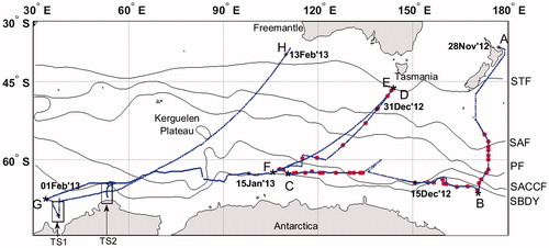
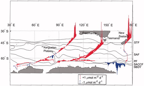
Oceanic and atmospheric CH₄ and CO₂ measurements were made quasi-continuously onboard R/V Mirai (Japan Agency for Marine-Earth Science and Technology) during the Pacific and Indian sectors of scientific cruise MR12-05 (legs 2 and 3) in the Southern Ocean from late November 2012 to mid-February 2013 (Fig. 1). Along the cruise track, we determined the geographical position of each oceanic front on the basis of vertical profiles of temperature and salinity (Orsi et al., 1995; Rintoul et al., 1997; Rintoul and Bullister, 1999; Yaremchuk et al., 2001), SST, and sea surface salinity (SSS) (Chaigneau and Morrow, 2002). The cruise included a zonal transect along the World Ocean Circulation Experiment Hydrographic Program line S4 and four meridional transects.

Fig. 1. Dash-dotted blue line shows the cruise track of R/V Mirai where underway measurements of oceanic CO₂ and CH₄ were made simultaneously. Red circles show hydrographic stations for measurements of CH₄ in discrete water samples (measurement system is described in Supplemental data). Black solid line shows the oceanic fronts from Orsi et al. (1995), and TS1 and TS2 coastal transects at 38^oE and 53.5^oE, respectively.

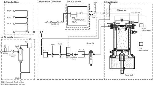
Underway measurements of CH₄ and CO₂ mixing ratios in dry air equilibrated with seawater (xCH₄^eq) and ambient air (xCH₄^air) were obtained with a system consisting of a cavity ring-down spectroscopy analyzsr (CRDS G2301, Picarro, Inc., Santa Clara, CA) and a shower-head type equilibrator that has been used for measurement of the partial pressure of CO₂ in seawater and overlying air since the late 1960s (Körtzinger et al., 2000; Yoshikawa-Inoue, 2000; Yoshikawa-Inoue and Ishii, 2005) (Fig. 2). Seawater was pumped from a water inlet ∼5 m below the sea surface at the bow of the ship to an onboard laboratory for measurement of CO₂ and CH₄, salinity, dissolved oxygen, and fluorescence (data available in R/V Mirai Cruise Report MR12-05). Sampled seawater was continuously introduced into the equilibrator at 10 L/min. Seawater temperature in the equilibrator was measured continuously with a PT-100 sensor. During the cruise, the increase of water temperature from the water inlet to the equilibrator was between 0.1 °C (at low latitudes) and 0.4 °C (at high latitudes). Air equilibrated with seawater was drawn continuously from the outlet of the equilibrator, then flowed into the CRDS analysers (100 mL/min), and was then returned to the equilibrator. Sample air was circulated within a closed loop during measurements of oceanic CO₂ and CH₄. To avoid band broadening effects caused by water vapor (Nara et al., 2012), water vapor was removed from the sample air by two electric dehumidifiers that use the Peltier effect, Nafion tubing (Perma Pure LLC, Lakewood, NJ), and a chemical desiccant column (Mg(ClO₄)₂). Equilibration pressure was assumed to be atmospheric pressure because the seawater inlet in the onboard laboratory was at atmospheric pressure.

Fig. 2. Schematic diagram of underway system for measurements of CO₂ and CH₄, consisting of a CRDS analyser and a shower-head-type equilibrator.

The CRDS analyser was calibrated daily with three CH₄ and CO₂ reference gases (1606.2, 1876.5, and 2075.1 ppb for CH₄; 249.23, 380.78, and 444.14 ppm for CO₂); the CH₄ data are traceable to the World Meteorological Organization CH₄ mole fraction scale (Dlugokencky et al., 2005; Tsuboi et al., 2016). The CRDS analyser produced about 100 digital analyses per minute from which we calculated and used one-minute means. We discarded data recorded for at least 30 min immediately after the changes in flow patterns during measurements of reference gases and ambient air. Based on replicated measurements of a sample gas in the cylinder, the precision of the analyses (±1σ) were estimated to be better than 0.1 ppm and 2 ppb for CO₂ and CH₄, respectively.

Although both CO₂ and CH₄ were measured simultaneously during the cruise, we focused in this study on the CH₄ distribution, the factors controlling the CH₄ distribution, and the sea–air flux of CH₄. CH₄ concentrations in surface seawater (C_w) and the mixing ratio in dry air of CH₄ equilibrated with surface seawater (xCH₄^sw) were calculated by using the temperature and salinity dependence of CH₄ solubility in seawater (Wiesenburg and Guinasso, 1979) and the barometric pressure at the sea surface (P_bar). The partial pressure of CH₄ in surface seawater (pCH₄^sw) was calculated as (1a) $${pCH}_4^{sw}={xCH}_4^{sw}(P_{bar}-W)$$(1a)

Similar to C_w calculations, however, CH₄ concentrations in the ambient ($C_a$) and the mixing ratios of CH₄ in the ambient air (${xCH}_4^a)$ were calculated by using equilibrium temperature and salinity dependence of equilibirum CH₄ solubility upper the surface seawater. The partial pressure of CH₄ upper the surface seawater (${pCH}_4^a$) was calculated as (1b) $${pCH}_4^a={xCH}_4^a(P_{bar}-W)$$(1b)

The saturation ratios (SR) of dissolved CH₄, which is the ratio of the C_w to the CH₄ concentration in seawater equilibrated with ambient air (C_a), is given by (2) $$\mathrm{SR}\text{(\%)} \text{=} \frac{C_w}{C_a}\times 100$$(2)

SR < 100% indicates water that is undersaturated relative to the atmosphere, and SR > 100% indicates supersaturation; SR is not affected by barometric pressure. The sea–air flux of CH₄ (F) was calculated as (3) $$F=k\times S\times \left({pCH}_4^{sw}-{pCH}_4^{air}\right)=k\times \left(C_w-C_a\right),$$(3) where S is CH₄ solubility in seawater and k is the gas transfer piston velocity calculated by the method of Wanninkhof (2014) as (4) $$k=0.251〈U_{10}^2〉{(Sc/660)}^{-0.5}$$(4)

Here, $〈U_{10}^2〉$ is wind speed 10 m above the sea surface, and Sc is the Schmidt number of CH₄ in seawater. We used ship-measured wind speed recorded by anenometer (model KE-500; Koshin Denki, Meguro-ku,Tokyo) to estimate in situ sea–air flux of CH₄.

SST, SSS (derived from conductivity), and dissolved oxygen (for determining AOU) were measured in surface seawater collected at 1 min intervals by a continuous sea surface water monitoring system (Marine Works Japan Co., Ltd., Oppamahigashi, Yokosuka). SST and SSS were measured with a thermosalinograph (SBE-45; Sea-Bird Electronics, Inc., Bellevue, WA) and dissolved oxygen with an optode (model 3835; Aanderaa Data Instruments, Bergen, Norway). Precisions for these measurements were SST ± 0.002 °C, SSS ± 0.0003 Sm⁻¹, and dissolved oxygen <8 µmol L⁻¹, respectively. Chlorophyll-a (chl-a) concentration was determined by the fluorescence of the extracted samples measured by a fluorometer (model 10-AU-005, Turner Designs) which was previously calibrated with pure chlorophyll a (Sigma-Aldrich Co., LLC, St. Louis, MO).

To evaluate total F in the Southern Ocean, we obtained gridded data (1° lat × 1° long) of SR by using long-term monthly means of AOU, SST, and sea-surface salinity (SSS) data (World Ocean Atlas, 2013; http://www.nodc.noaa.gov/OC5/woa13/). Monthly means of C_w were obtained from SR and the CH₄ mixing ratio in xCH₄^air measured on board the ship. Monthly means of wind speed were taken from ERA-Interim global reanalysis data (0.5° lat × 0.5° long; European Centre for Medium-range Weather Forecasts, http://www.ecmwf.int/en/research/climate-reanalysis/era-interim). Total CH₄ emissions in the Southern Ocean were calculated as (5) $$\mathrm{T}\mathrm{o}\mathrm{t}\mathrm{a}\mathrm{l}\mathrm{ }{\mathrm{C}\mathrm{H}}_4\mathrm{ }\mathrm{e}\mathrm{m}\mathrm{i}\mathrm{s}\mathrm{s}\mathrm{i}\mathrm{o}\mathrm{n}\mathrm{s}=\sum _{i=1}^n\left(F_i\times {SA}_i\right)$$(5) where subscript i is grid number and SA is the surface area within a grid where the sea surface is free of sea ice. In this study, we assumed no CH₄ exchange across the air–sea interface where there is sea ice. Monthly long-term sea-ice concentration data (1.875° lat × 1.905° long) were taken from NCEP/NCAR reanalysis data (Kalnay et al., 1996).

4. Results

4.1. Meridional distribution of CH₄ in surface seawater

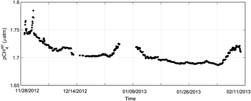
First we examined temporal variations of atmospheric CH₄ in the Southern Hemisphere to confirm that the atmospheric CH₄ mixing ratios measured by the CRDS analyser were accurate. During the cruise, the mean of atmospheric xCH₄^air was 1775.9 ± 5.4 ppb (n = 33) in late November 2012, 1767.2 ± 5.4 ppb (n = 321) in December 2012, 1755.7 ± 2.0 ppb (n = 304) in January 2013, and 1751.0 ± 1.5 ppb (n = 150) in early February 2013, and showed the same seasonal variations as reported for the Southern Hemisphere by Dlugokencky et al. (1994) (Fig. 3). Mean values in December 2012 and January 2013 agreed well (within 5 ppb) with monthly means at Cape Grim (40.68°S, 144.69°E), Tasmania, and at the South Pole, on the basis of data from the NOAA/ESRL network (http://www.esrl.noaa.gov/gmd/ccgg/trends_ch4/).

Fig. 3. Atmospheric CH4 mixing ratios measured by CRDS analyser during the cruise track of R/V Mirai.

The meridional distribution of pCH₄^sw between New Zealand and the SBDY (63.5^oS) (Fig. 4) showed a few pCH₄^sw peaks of up to 3.4 µatm and an SR range from 100% to 185% in the coastal area off New Zealand. These peaks can be attributed in part to CH₄ that is produced by methanogenesis in buried sediment layers in productive coastal areas (Scranton and McShane, 1991; Hovland et al., 1993; Grunwald et al., 2009). CH₄ inputs from riverine and groundwater discharge can also contribute to CH₄ supersaturation in coastal areas (Bugna et al., 1996; Kim and Hwang, 2002; Reeburgh, 2007). In surface seawater off the New Zealand coast, strong pCH₄^sw peaks are accompanied by lower water density (lower SSS), which reflects input of fresh water with high CH₄.

Fig. 4. Meridional distribution of pCH₄^air, pCH₄^sw, chl-a, AOU, SST, SSS, SR along transect from offshore New Zealand to Antarctica (A–B).

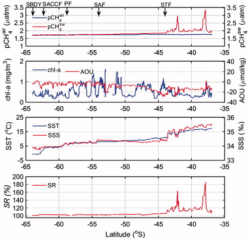
Fig. 5. Meridional distribution of pCH₄^air, pCH₄^sw, chl-a, AOU, SST, SSS, SR from SBDY to SAF during northbound sailing to Tasmania (Leg 2) (C–D).

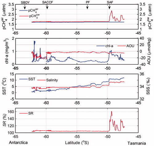
In the open ocean area from the STF (44°S) to the SBDY (63.5°S) (Fig. 4), pCH₄^sw decreased slightly and monotonously to the south and SR decreased from 119% to 100%; both of these results agree well with those of earlier studies (Bates et al., 1996; Kelley and Jeffrey, 2002). Atmospheric CH₄ has increased by 180 ppb (about 10%) between 1984 and 2012, although the rate of increase was slower between 1999 and 2006 (Dalsøren et al., 2016; McNorton et al., 2016). The fairly constant SR over these few decades suggests parallel increases of pCH₄^sw and pCH₄^air. South of the SBDY (63.5°S), pCH₄^sw decreased considerably along with decreases in SST and chl-a concentration and an increase in AOU. The lowest value of SR that we observed (85%) was in this region.

South of the STF, pCH₄^sw changed little (Fig. 4), but there were steep changes in SST and SSS at each of the other fronts. Because CH₄ solubility is a function of SST and SSS (Wiesenburg and Guinasso, 1979), the relatively constant pCH₄^sw indicates that there must have been changes in C_w at each front. According to Wiesenburg and Guinasso (1979; their equation 7), CH₄ solubility decreases approximately by 2.3% for each unit increase in SST above 10 °C at constant SSS (34), and roughly by 0.8% for each unit increase in SSS from 34 at constant SST (10 °C). The decreases of SST and SSS to the south caused large increases of C_w to the south.

The meridional variations of pCH₄^sw during the sections of the cruise sailing toward and away from southern Tasmania, and during the northbound section sailing toward Fremantle (Fig. 1 and 5–7), were similar to those between the STF and the SBDY between New Zealand and Antarctica (Fig. 4). During the northbound sailing to Tasmania, pCH₄^sw varied considerably between 1.8 and 2.9 µatm north of the SAF (49.5°S). Strong pCH₄^sw peaks that continued over several tens of kilometers coincided with increases in chl-a concentration. However, about one week after the northbound sailing toward Tasmania we found no strong peaks of pCH₄^sw at the same geographical positions (Fig. 6). During the northbound sailing to Fremantle, pCH₄^sw north of the STF also varied considerably, from 1.8 to 2.7 µatm, but without correlation with chl-a concentration, SST, or SSS (Fig. 7). Thus, it appears that none of the other quantities we determined in this study can be reliably used to predict strong peaks of pCH₄^sw north of the STF.

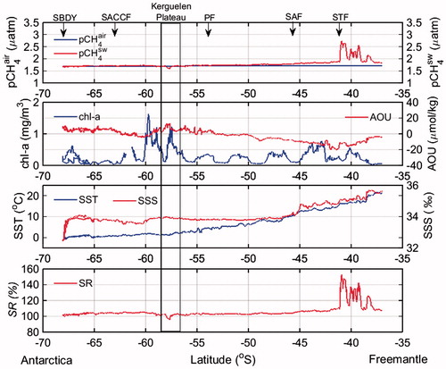
Fig. 6. Meridional distribution of pCH₄^air, pCH₄^sw, chl-a, AOU, SST, SSS, SR from STF to SBDY during southbound sailing (Leg 3) (E–F).

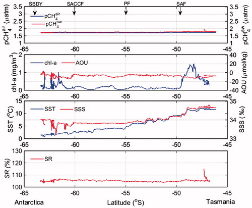
Fig. 7. Same as in Fig. 6 except from SBDY to STF during northbound sailing to Fremantle (Leg 3) (G–H).

4.2. Zonal distribution of CH₄ in surface seawater at high latitudes

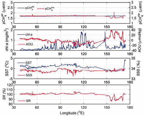
The pCH₄^air at latitudes south of 60°S (Fig. 8) decreased westward, which was a response to seasonal variations in atmospheric CH₄ and decreases in barometric pressure. As noted above (see discussion of Fig. 4), pCH₄^sw east of 140°E decreased considerably, along with decreases in SST and chl-a and increases in AOU (Fig. 4). Holm-Hansen et al. (2005) reported that in a relatively shallow area of the Southern Ocean bounded by 145° to 170°E and 62° to 66°S, where the bottom topography is complex and there are numerous islands, banks, and seamounts, upwelling of deep water creates regions of high-chlorophyll pelagic seawater. In very early December, which is before the onset of strong biological activity, we observed positive AOU (41 µmol kg⁻¹) and low chl-a concentrations in this region.

Fig. 8. Zonal distribution of pCH₄^air, pCH₄^sw, chl-a, AOU, SST, SSS, SR south of 60°S (B–C–G).

4.3. Sea–air flux of CH₄

The pCH₄^sw and pCH₄^air data we acquired along the cruise track allowed us to use Equation (3)(3) $$F=k\times S\times \left({pCH}_4^{sw}-{pCH}_4^{air}\right)=k\times \left(C_w-C_a\right),$$(3) to calculate the sea–air flux of CH₄ over a wide area of the Southern Ocean (Fig. 9). The flux of CH₄, we determined, ranged from –3.9 to 8.5 µmol m⁻²day⁻¹ (average 0.19 µmol m⁻²day⁻¹) and was largest and most variable at lower latitudes, especially off New Zealand. In the pelagic zone between the SAF and SBDY, it ranged from –0.43 to 0.50 µmol m⁻² d⁻¹ and there was CH₄ uptake by surface seawater in the area of the Kerguelen Plateau. We observed intermittent pCH₄^sw peaks north of the SAF and STF (see section ‘Meridional distribution of CH₄ in surface seawater’) that led to higher sea–air flux of CH₄ there. It is important to examine the triggers of these strong pCH₄^sw peaks at lower latitudes in our evaluation of oceanic CH₄ flux. In the area south of the SBDY and east of 140°E, our data (Fig. 9) show that surface seawater there acts as a net sink for atmospheric CH₄ during the cruise.

Fig. 9. The CH₄ flux along the cruise track (red color indicates CH₄ release, and blue color indicates CH₄ uptake in seawater).

5. Discussion

The minimum pCH₄^sw we observed was over the Kerguelen Plateau, where it corresponded to local variations of other parameters: a decrease in SST, a slightly positive AOU (5 µmol kg⁻¹), and elevated chl-a concentration. Gille et al. (2014) reported that cold SSTs in the Kerguelen region correlate with high wind speeds, and that wind-mixing of the upper ocean there resulted in entrainment of cold water into the mixed layer and euphotic zone. Mashayek et al. (2017) also identified spatiotemporal changes of mixing of waters in a shallow region of the Southern Ocean by using trifluoromethyl sulfur pentafluoride (CF₃SF₅) as a passive chemical tracer. In the Southern Ocean, strong vertical mixing is induced by near-surface westerly winds that cause convergent flow at intermediate depths; such mixing partially offsets upwelling (Marshall and Speer, 2012). The fluxes of greenhouse gases there between air and sea and those in the water column are affected not only by physical processes, but also by the availability of organic matter and oxygen (Codispoti et al., 2001). CH₄ is formed mainly by methanogens (Wuebbles and Hayboe, 2002) during anaerobic degradation of organic matter or by the transformation of methyl compounds by methylotrophs (Damm et al., 2008), whereas CH₄ consumption occurs as a result of aerobic methanotrophy (Hanson and Hanson, 1996). In the region between the PF (58.5°S) and the SBDY, C_w tended to be high, suggesting enhancement of biogenic CH₄ production (Heeschen et al., 2004), lower rates of CH₄ oxidation and CH₄ flux between the sea and overlying air, or both. In this region, vertical mixing has been reported to support the development of chl-a blooms (Gille et al., 2014) and high AOU values. AOU is respiration in the ocean interior (without contact with the atmosphere), where lower concentrations of CH₄ would be expected because of its removal by oxidation, by upwelling of old deep water with low CH₄ concentrations, or both (Heeschen et al., 2004). Positive AOU values in surface seawater suggest that air–sea exchange of O₂ and O₂ production due to photosynthesis by phytoplankton were too slow to establish equilibrium after or during vertical mixing. Because maximum CH₄ concentrations at high latitudes south of the PF are in surface waters and decrease with depth (therefore there are no subsurface CH₄ maxima) (Yoshida et al., 2011), we would expect a negative relationship between pCH₄^sw and AOU.

Lowering of pCH₄^sw is to be expected with increasing AOU, as was evident over the Keruguelen Plateau (Fig. 7), which is consistent with higher AOU than surrounding (Aoki et al., 2007). Aoki et al. (2007) reported that cyclonic eddies of 100–150 km diameter appear every year in a particular area at around 140°E, and that the properties of the water in the eddies are similar to those of water over the continental slope. Large-scale spatial variability of pCH₄^sw might be caused by physical processes such as upwelling. West of 140°E, surface seawater CH₄ almost equilibrated to atmospheric CH₄ (SR = 100.04%) (Fig. 8), except at high latitudes along 38°E and 53.5°E (TS1 and TS2, respectively) where SST was lower than 0 °C and AOU was positive (Fig. 9a,b). The resultant shallow stratification can trap organisms in the sunlit (productive) layer. Although phytoplankton do not generate CH₄ directly, the high CH₄^sw concentrations there is probably a result of Antarctic krill, zooplankton, or both feeding on phytoplankton and the subsequent microbial methanogenesis (Yoshida et al., 2011).

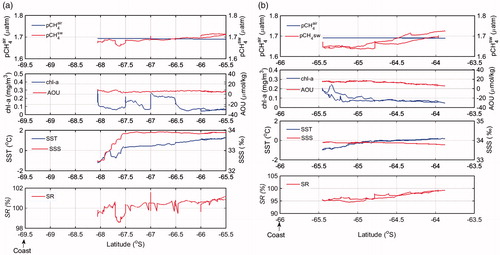
South of the ASF along 38°E and 53.5°E (at 67.5°S and 64.5°S along coastal TS1 and TS2, respectively), pCH₄^sw decreased toward the continent (Fig. 10a) within the range from 1.65 to 1.69 µatm. The ASF is a strong horizontal subsurface temperature front defined by the 0 °C isotherm (Ainley and Jacobs, 1981) and clearly separates the cold and shelf waters from the modified CDW, which can extend all the way to onto the Antarctic Shelf (Williams et al., 2010). Along 53.5°E (TS2, Fig. 10b), pCH₄^sw also decreased southward, accompanied by an increase in AOU, which is the same pattern as that we observed east of 140°E and over the Kerguelen Plateau. The coastward decreases of pCH₄^sw that we observed (TS1 and TS2), which are caused by local dynamic mechanisms such as low SST and AOU, might also reflect the lack of both a CH₄ subsurface maximum and a sediment source. The coastward decrease of pCH₄^sw is the opposite trend to that observed in tropical and extratropical regions. In the Antarctica, the physical features are the same, either mixing or upwelling; but the upwelled water is distinct. Upwelling of old CH₄-poor water characterised by former biological oxidation (Rehder et al., 1999) and/or by contact with a former atmosphere with low methane content off Antarctica (Heeschen et al., 2004), versus upwelled water in the tropics and subtropics fed by depleted oxygen subsurface water and potentially contact with organic-rich sediments (Reeburgh, 2007).

Fig. 10. Meridional distribution of pCH₄^air, pCH₄^sw, chl-a, AOU, SST, SSS, SR at (a) transect 1 (38°E); (b) transect 2 (53.5°E). An arrow at the bottom indicates the position of the coast.

The CH₄ flux data we have determined is limited to the course of cruise MR12-05. To gain a good understanding of the oceanic CH₄ cycle throughout the South Pacific and Southern Ocean, we need a much greater geographic spread of data. This might be achieved by using variables such as SST and chl-a concentration, which are related to the distribution of SR (and hence to pCH₄^sw), and are measured remotely over wide areas. If such relationships exist between SR and other oceanographic processes it would then be relatively simple to interpolate or extrapolate observed SR values across the Southern Ocean, which would allow a more precise evaluation of the sea–air flux of CH₄. Biological activity (CH₄ production and oxidation), ocean dynamics (lateral flow, vertical mixing, and upwelling), CH₄ solubility, and the sea–air flux of CH₄ have a major effect on the spatiotemporal variation of SR. Based on the assumption that these factors are directly or indirectly related to SR, we investigated possible relationships between SR at high latitudes (south of 50°S) and SST, chl-a, water density, and AOU.

First, we examined the SR–SST relationship south of 50°S (taken to be south of the PF). SR increased dramatically with only slight increases in SST (at around 0 °C) (Fig. 11). Although we found no clear relationship between SR and chl-a, such a relationship may exist within areas much smaller than our study area (Damm et al., 2008; Yoshida et al., 2011). Yoshida et al. (2011) reported a strong relationship between C_w and seawater density in the South Pacific – Southern Ocean region, but this relationship does not hold in regions of low SST. While cruising at high latitudes from December 2012 to February 2013, we noted a possible correlation between pCH₄^sw and AOU, which we investigated further (Fig. 12). The resultant analysis of data collected along the cruise track in the open ocean south of 50°S shows that the following linear relationship between SR and AOU applies, at least in the Southern Ocean south of 50°S: (6) $$SR=-0.294\times AOU+100.093\mathrm{ }(r^2=0.89,\mathrm{ }n=1549)$$(6)

Fig. 11. The relationship between SR and SST south of 50°S in the Southern Ocean (n = 1549).

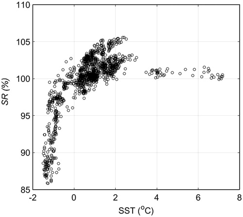
Fig. 12. The relationship between SR and AOU south of 50^oS in the Southern Ocean. Solid line shows the linear relationship between SR and AOU: SR = −0.294 × AOU + 100.093 (r² = 0.89, n = 1549).

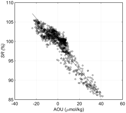
We got a good correlation between AOU and SR (Equation (6)(6) $$SR=-0.294\times AOU+100.093\mathrm{ }(r^2=0.89,\mathrm{ }n=1549)$$(6) ). In the subsurface water which is brought upward by vertical mixing, is characterised by positive AOU and low ${pCH}_4^{sw}$ (Heeschen et al., 2004). At the sea–air interface, the transfer velocity for gas exchange of oxygen and CH₄ is quite similar, it means that undersaturation due to on the same timscale. The correlation here is also a strong indication for lacking of importance of biological production.

To obtain a map of the distribution of the sea–air flux of CH₄ in the Southern Ocean south of 50°S, we first determined the distribution of SR by applying Equation (6)(6) $$SR=-0.294\times AOU+100.093\mathrm{ }(r^2=0.89,\mathrm{ }n=1549)$$(6) to the long-term monthly mean AOU data (1° × 1° grid) for December, January, and February from the World Ocean Atlas (Garcia et al. 2014). Because monthly mean AOU data for each year are not available, so we estimated a SR distribution based on climatological AOU data. Then, we calculated the monthly mean sea–air flux of CH₄ and total CH₄ emission for the three months (Table 1 and Fig. 13). The sea–air flux of CH₄ is controlled mainly by C_w – C_a (see Equation (3)(3) $$F=k\times S\times \left({pCH}_4^{sw}-{pCH}_4^{air}\right)=k\times \left(C_w-C_a\right),$$(3) ) and wind speed, and total CH₄ emission in the Southern Ocean is controlled by the sea–air flux of CH₄ and the amount of sea-ice coverage. Although the AOU data for each grid cell suggest strong uptake of CH₄ in seawater in December, the area of surface seawater in contact with the atmosphere is small at higher latitudes in December due to sea-ice coverage. Although the AOU data suggest that CH₄ uptake in the Weddell Sea and Ross Sea would be considerable, these areas are largely covered by sea ice in December. From December to January, total CH₄ emission increased by 0.014 Tg yr⁻¹ owing to an increase in sea–air flux of CH₄ and the retreat of sea ice. Following the retreat of the sea ice, CH₄ flux tended to be higher slightly south of the sea ice and the coastal region showed a large negative sea–air flux of CH₄ (CH₄ uptake). From January to February total net CH₄ evasion decreased by 44% (0.02 Tg yr⁻¹) while both the area of surface in contact with the ambient air and the wind speed increased. In February, CH₄ flux was generally small in the area south of the edge of the sea ice. Surface seawater between 50° and 60°S, which is a region of high wind speed, was a source of atmospheric CH₄ from December to February. The CH₄ flux obtained from gridded AOU data along the cruise track (south of 50°S) was in the range from –2.4 to 2.1 µmol m⁻² d⁻¹ (mean 0.08 µmol m⁻² d⁻¹), which is lower than that obtained from our underway measurements (0.194 µmol m⁻² d⁻¹); we attribute the difference to the effect of strong winds during the cruise, especially near 50°S. In coastal regions, the higher CH₄ fluxes obtained from gridded AOU data might also reflect local variations of AOU and coastal dynamic mechanisms, which may have contributed to these higher fluxes. Thus, there are limitations to the use of Equation (6)(6) $$SR=-0.294\times AOU+100.093\mathrm{ }(r^2=0.89,\mathrm{ }n=1549)$$(6) to extrapolate CH₄ fluxes across the entire Southern Ocean.

Fig. 13. Monthly mean sea-air CH₄ flux in the Southern Ocean from December to February (from upper panel to bottom panel). White areas is sea ice coverage.

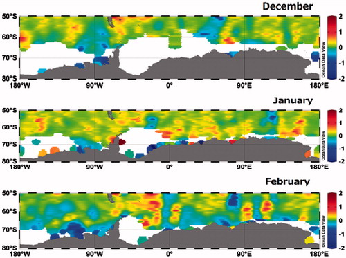
Table 1. Monthly mean AOU, wind speed, sea-air CH₄ flux in the Southern Ocean (south of 50°S).

	Dec	Jan	Feb	Average
Mean AOU (µmol kg^−1)	−2.5	−3.2	−0.1	−1.9
CH4 saturation ratios (SR, %)	100.84	101.04	100.13	100.67
Mean wind speed (U, m s^−1) (avg 30 years)	6.9	6.78	7.44	7.03
CH4 flux (µmol m^−2 day^−1)	0.09	0.14	0.06	0.08
CH4 emission (Tg yr^−1)	0.027	0.04	0.019	0.024

South of 50°S, the average CH₄ flux in austral summer is 0.024 Tg yr⁻¹, which accounts for a minor contribution of oceanic release CH₄ to the atmosphere (4–15 Tg yr⁻¹, IPCC, 2007). Considering that the area the Southern Ocean south of 50°S represents 13% of the global oceanic area, this efflux seems very small, but we attribute it to the high invasion of CH₄ at high latitudes. Although we have treated sea ice as an impermeable barrier to sea–air exchange of CH₄ in this study, recent studies suggest that gas exchange through sea ice does occur (Nomura et al., 2010, 2013, 2014). The estimates of CH₄ flux derived from the AOU–SR relationship is the main highlight of this study: this relationship can be extrapolated to apply at least to the entire Southern Ocean. To improve predictions of future changes of the global sea–air flux of CH₄, more observation data are required in areas where these fluxes are most variable, in particular, in the Southern Ocean in areas of seasonal sea ice coverage, in tropical and extratropical coastal regions, and in marginal seas.

6. Summary

We used a CRDS system coupled with a shower-head type equilibrator to obtain quasi-continuous underway measurements of the mixing ratio of oceanic CH₄ in seawater during legs 2 and 3 of cruise MR12-05 of R/V Mirai in the Southern Ocean from late November 2012 to mid-February 2013. Our pCH₄^sw data show that surface seawater was supersaturated with CH₄ in the tropics and extratropics, but both super- and undersaturated at high latitudes. Undersaturation occurred in areas where SST was low (<0 °C), AOU was positive (up to 41 µmol/kg), and chl-a concentrations were low (<0.3 mg/L), indicating that these areas were affected by upwelling and vertical mixing and limited biological production of CH₄. The SR in our entire dataset ranged from 85 to 185% (average 104 ± 4%). High SR in the north is biased due to coastal vicinity.

To attempt a regional evaluation of the sea–air flux of CH₄ over a wide area of Southern Ocean, beyond the limits imposed by using data only from the course of R/V Mirai, we examined the relationships of SR (hence pCH₄^sw) with several other oceanographic variables that are being measured remotely over wide areas. For the area south of the PF (50°S), we identified a strong linear relationship between SR and AOU that indicates that vertical mixing and upwelling are important factors that influence the spatial distribution of oceanic CH₄. On the basis of this linear relationship, we calculated the regional climatological distribution of the sea–air flux of CH₄ in the Southern Ocean south of 50°S for the period from December to February. We estimated emissions of CH₄ from the Southern Ocean to be 0.03 Tg yr⁻¹ in December, 0.04 Tg yr⁻¹ in January, and 0.02 Tg yr⁻¹ in February. Total CH₄ emissions increased from December to January in response to the combined effect of an increase in sea–air flux of CH₄ and retreat of seasonal sea ice. From January to February, total CH₄ emissions decreased because the sea–air flux of CH₄ decreased as a result of declines in both wind speed and the area of sea surface in contact with ambient air (increase in sea ice). Although the effect of CH₄ emissions from the Southern Ocean has limited global impact, our results clearly show climatological variations of the sea–air flux of CH₄ in the Southern Ocean from December to February.

Supplemental data

Supplemental data for this article can be accessed here: https://doi.org/10.1080/16000889.2018.1478594.

Acknowledgements

We greatly appreciate the shipboard support of the master and crew of R/V Mirai during legs 2 and 3 of cruise MR12-05. This research was supported in part by the GRENE Project and by Grants-in-Aid for Scientific Research from the Ministry of Education, Culture, Sports, Science and Technology of Japan (#23241002, #26281001). We thank Dr Shigeru Aoki for his insightful comments and helpful suggestions.

Disclosure statement

No potential conflict of interest was reported by the authors.

References

- Ainley, D. and Jacobs, S. 1981. Seabird affinities for ocean and ice boundaries in the Antarctic. Deep Sea Res. 28, 1173–1185. DOI:10.1016/0198-0149(81)90054-6.
- Aoki, S., Fukai, D., Hirawake, T., Ushio, S., Rintoul, S. R. and co-authors. 2007. A series of cyclonic eddies in the Antarctic Divergence off Adélie Coast. J. Geophys. Res. 112, C05019. DOI:10.1029/2006JC003712.
- Bange, H. W., Bartell, U. H., Rapsomanikis, S. and Andreae, M. O. 1994. Methane in the Baltic and North Seas and a reassessment of the marine emissions of methane. Global Biogeochem. Cycles 8, 465–480.
- Bates, T. S., Kelly, K. C. and Johnson, J. E. 1993. Concentrations and fluxes of dissolved biogenic gases (DMS, CH4, CO, CO2) in the Equatorial Pacific during the SAGA-3 experiment. J. Geophys. Res. Atmos. 98, 16969–16977. DOI:10.1029/93JD00526.
- Bates, T. S., Kelly, K. C., Johnson, J. E. and Gammon, R. H. 1996. A reevaluation of the open ocean source of methane to the atmosphere. J. Geophys. Res. Atmos. 101, 6953–6961. DOI:10.1029/95JD03348.
- Bugna, G. C., Chanton, J. P., Cable, J. E., Burnett, W. C. and Cable, P. H. 1996. The importance of groundwater discharge to the methane budgets of nearshore and continental shelf waters of the northeastern Gulf of Mexico. Geochim. Cosmochim. Acta. 60, 4735–4746.
- Burke, R. A., Reid, D. F., Brooks, J. M. and Lavoie, D. M. 1983. Upper water column methane geochemistry in the eastern tropical North Pacific. Limnol. Oceanogr. 28, 19–32.
- Callahan, J. E. 1972. Structure and circulation of deep water in Antarctic. Deep Sea Res. 19, 563–575.
- Chaigneau, A. and Morrow, R. 2002. Surface temperature and salinity variations between Tasmania and Antarctica, 1993–1999. J. Geophys. Res. 107, SRF 22-1. DOI:10.1029/2001JC000808.
- Cicerone, R. J. and Oremland, R. S. 1988. Biogeochemical aspects of atmospheric methane. Global Biogeochem. Cycles 2, 299–327.
- Codispoti, L. A., Brandes, J. A., Christensen, J. P., Devol, A. H., Naqvi, S. W. A. and co-authors. 2001. The oceanic fixed nitrogen and nitrous oxide budgets: moving targets as we enter the anthropocene? Sci. Mar. 65, 85–105.
- Conrad, R. and Seiler, W. 1988. Methane and hydrogen in seawater (Atlantic Ocean). Deep Sea Res. A. 35, 1903–1917.
- Crutzen, P. J. and Zimmermann, P. H. 1991. The changing photochemistry of the troposphere. Tellus A. 43, 136–151.
- Dalsøren, S. B., Myhre, C. L., Myhre, G., Gomez-Pelaez, A. J., Søvde, O. A. and co-authors. 2016. Atmospheric methane evolution the last 40 years. Atmos. Chem. Phys. 16, 3099–3126. DOI:10.5194/acp-16-3099-2016.
- Damm, E., Kiene, R. P., Schwarz, J., Falck, E. and Dieckmann, G. 2008. Methane cycling in Arctic shelf water with phyotoplankton biomass and DMSP. Mar. Chem. 109, 45–59.
- De Angelis, M. A. and Lee, C. 1994. Methane production during zooplankton grazing on marine-phytoplankton. Limnol. Oceanogr. 39, 1298–1308.
- Dlugokencky, E. J., Masaire, K. A., Lang, P. M., Tans, P., Steele, L. P. and co-authors. 1994. A dramatic decrease in the growth rate of atmospheric methane in the Northern Hemisphere during 1992. Geophys. Res. Lett. 21, 45–48.
- Dlugokencky, E. J., Myers, R. C., Lang, P. M., Masarie, K. A., Crotwell, A. M. and co-authors. 2005. Geophys. Res. 110, D18306. DOI:10.1029/2005JD006035.
- Fischer, G., Futterer, B., Gersonde, R., Honjo, S., Ostermann, D. and co-authors. 1988. Seasonal variability of particle flux in the Weddell Sea and its relation to ice cover. Nature 335, 426–428.
- Garcia, H. E., Locarnini, R. A., Boyer, T. P., Antonov, J. I., Baranova, O.K. and co-authors. 2014. World Ocean Atlas 2013, Volume 3: Dissolved oxygen, apparent oxygen utilization, and oxygen saturation. In: NOAA Atlas NESDIS 75 (ed. S. Levitus, Technical ed. A. Mishonov), 27 pp.
- Georgi, D. T. 1981. On the relationship between the large-scale property variations and fine-structure in the Circumpolar Deep Water. J. Geophys. Res. Oceans. 86, 6556–6566.
- Gille, S. T., Carranza, M. M., Cambra, R. and Morrow, R. 2014. Wind-induced upwelling in the Kerguelen Plateau region. Biogeosciences 11, 6389–6400. DOI:10.5194/bg-11-6389-2014.
- Grunwald, M., Dellwig, O., Beck, M., Dippner, J. W., Freund, J. A. and co-authors. 2009. Methane in the southern North Sea: sources, spatial distribution and budgets. Estuar. Coast. Shelf Sci. 81, 445–456.
- Hanson, S. R. and Hanson, E. T. 1996. Methanotrophic bacteria. Microbiol. Rev. 60, 439–471.
- Heeschen, K. U., Keir, R. S., Rehder, G., Klatt, O. and Suess, E. 2004. Methane dynamics in the Weddell Sea determined via stable isotope ratios and CFC-11. Global Biogeochem. Cycles 18, GB2012. DOI:29/2003GB002151.
- Holm-Hansen, O., Kahru, M. and Hewes, C. D. 2005. Deep chlorophyll a maxima (DCMs) in pelagic Antarctic waters. II. Relation to bathymetric features and dissolved iron concentrations. Mar. Ecol. Prog. Ser. 297, 71–81.
- Hovland, M., Judd, A. G. and Burke, R. A. J. 1993. The global flux of methane from shallow submarine sediments. Chemosphere 26, 559–578.
- IPCC. 2007. Climate change 2007: the physical science basis. In: Contribution of Working Group I to the Fourth Assessment Report of Intergovernmental Panel on Climate Change (eds. S. Solomon, D. Qin, M. Manning, Z. Chen, M. Marquis, et al.) Cambridge University Press, Cambridge, 996 pp.
- James, H. E., Bousquet, P., Bussmann, I., Haeckel, M., Kipfer, R. and co-authors. 2016. Effects of climate change on methane emissions from seafloor sediments in the Arctic Ocean: a review. Limnol. Oceanogr. 61, S283–S299. DOI:10.1002/lno.10307.
- Körtzinger, A., Mintrop, L., Wallace, D. W. R., Johnson, K. M., Neill, C. and co-authors. 2000. The international at-sea intercomparison of fCO2 systems during the R/V Meteor Cruise 36/1 in the North Atlantic Ocean. Mar. Chem. 72, 171–192.
- Kalnay, E., Kanamitsu, M., Kistler, R., Collins, W., Deaven, D. and co-authors. 1996. The NCEP/NCAR 40-Year Reanalysis Project. Bull. Amer. Meteor. Soc. 77, 437–472.
- Karl, D. M. and Tilbrook, B. D. 1994. Production and transport of methane in oceanic particulate organic matter. Nature 368, 732–734.
- Kelley, C. A. and Jeffrey, W. H. 2002. Dissolved methane concentration profiles and air-sea fluxes from 41oS to 27oN. Global Biogeochem. Cycles 16, 13-1–40. DOI:10.1029/2001GB001809.
- Kim, G. and Hwang, D. W. 2002. Tidal pumping of groundwater into the coastal ocean revealed from submarine Rn-222 and CH4 monitoring. Geophys. Res. Lett. 29, 23-1. DOI:10.1029/2002GL015093.
- Knox, G. A. 2007. Biology of the Southern Ocean. Taylor & Francis Group, LLC, CRC Press, pp. 147–158.
- Lamontagne, R. A., Swinnert, J. W., Linnenbo, V. J. and Smith, W. D. 1973. Methane concentrations in various marine environments. J. Geophys. Res. 78, 5317–5324.
- Locarnini, R. A. 1994. Water Masses and Circulation in the Ross Gyre and Environs. PhD thesis, Texas A&M University, pp. 42–80.
- Marshall, J. and Speer, K. 2012. Closure of the meridional overturning circulation through Southern Ocean upwelling. Nature Geosci. 5, 171–180. DOI:10.1038/NGEO1391.
- Mashayek, A., Ferrari, R., Merrifield, S., Ledwell, J. R., St Laurent, L. and co-authors. 2017. Topographic enhancement of vertical turbulent mixing in the Southern Ocean. Nat. Comms. 8, 14197. DOI:10.1038/ncomms14197.
- McNorton, J., Chipperfield, M. P., Gloor, M., Wilson, C., Feng, W. and co-authors. 2016. Role of OH variability in the stalling of the global atmospheric CH4 growth rate from 1999 to 2006. Atmos. Chem. Phys. 16, 7943–7956. DOI:10.5194/acp-16-7943-2016.
- Nara, H., Tanimoto, H., Tohjima, Y., Mukai, H., Nojiri, Y. and cp-authors. 2012. Effect of air composition (N2, O2, Ar, and H2O) on CO2 and CH4 measurement by wavelength-scanned cavity ring-down spectroscopy: calibration and measurement strategy. Atmos. Meas. Tech. 5, 2689–2701.
- Nomura, D., Eicken, H., Gradinger, R. and Shirasawa, K. 2010. Rapid physically driven inversion of the air-sea ice CO2 flux in the seasonal landfast ice off Barrow, Alaska after onset of surface melt. Cont. Shelf Res. 30, 1998–2004.
- Nomura, D., Granskog, M. A., Assmy, P., Simizu, D. and Hashida, G. 2013. Arctic and Antarctic sea ice acts as a sink for atmospheric CO2 during periods of snow melt and surface flooding. J. Geophys. Res. Oceans. 118, 6511–6524.
- Nomura, D., Yoshikawa-Inoue, H., Kobayashi, S., Nakaoka, S., Nakata, K. and co-authors. 2014. Winter-to-summer evolution of pCO2 in surface water and air-sea CO2 flux in the seasonal ice zone of the Southern Ocean. Biogeosciences 11, 5749–5761.
- Orsi, A. H., Whitworth, T. and Nowlin, W. D. 1995. On the meridional extent and fronts of the Antarctic Circumpolar Current. Deep Sea Res. Part 1 Oceanogr. Res. Pap. 42, 641–673.
- Reeburgh, W. S. 2007. Oceanic methane biogeochemistry. Chem. Rev. 107, 486–513.
- Rehder, G., Keir, R. S., Suess, E. and Rhein, M. 1999. Methane in the northern Atlantic controlled by microbial oxidation and atmospheric history. Geophys. Res. Lett. 26, 587–590.
- Rintoul, S. R. and Bullister, J. L. 1999. A late winter hydrographic section from Tasmania to Antarctica. Deep Sea Res. Part 1 Oceanogr. Res. Pap. 46, 1417–1454.
- Rintoul, S. R., Donguy, J. R. and Roemmich, D. H. 1997. Seasonal evolution of upper ocean thermal structure between Tasmania and Antarctica. Deep Sea Res. Part 1 Oceanogr. Res. Pap. 44, 1185–1202.
- Saunois, M., Bousquet, P., Poulter, B., Peregon, A., Ciais, P. and co-authors. 2016. The global methane budget 2000-2012. Earth Syst. Sci. Data. 8, 697–751. DOI:10.5194/essd-8-697-2016.
- Scranton, M. I. and McShane, K. 1991. Methane fluxes in the southern North Sea: the role of European rivers. Cont. Shelf Res. 11, 37–52.
- Thornton, F. B., Geibel, C. M., Crill, M. P., Humborg, C. and Morth, C. M. 2016. Methane fluxes from the sea to the atmosphere across the Siberian shelf seas. Geophys. Res. Lett. 43, 5869. DOI:10.1002/2016GL068977.
- Tilbrook, B. D. and Karl, D. M. 1994. Dissolved methane distributions, sources, and sinks in the western Bransfield Strait, Antarctica. J. Geophys. Res. Oceans. 99, 16383–16393.
- Tilbrook, B. D. and Karl, D. M. 1995. Methane sources, distributions and sinks from California coastal waters to the oligotrophic North Pacific gyre. Mar. Chem. 49, 51–64.
- Tsuboi, K., Matsueda, H., Sawa, Y., Niwa, Y., Takahashi, M. and co-authors. 2016. Scale and stability of methane standard gas in JMA and comparison with MRI standard gas. Pap. Met. Geophys. 66, 15–24.
- Wanninkhof, R. 2014. Relationship between wind speed and gas-exchange over the ocean revisited. Limnol. Oceanogr. Methods. 12, 351–362.
- Whitworth, T. and Nowlin, W. D. 1987. Water masses and currents of the Southern Ocean at the Greenwich Meridian. J. Geophys. Res. Oceans 92, 6462–6476.
- Wiesenburg, D. A. and Guinasso, N. L. 1979. Equilibrium solubilities of methane, carbon-monoxide, and hydrogen in water and sea water. J. Chem. Eng. Data. 24, 356–360.
- Williams, G. D., Nicol, S., Aoki, S., Meijers, A. J. S., Bindoff, N. L. and co-authors. 2010. Surface oceanography of BROKE-West, along the Antarctic margin of the south-west Indian Ocean (30-80 degrees E). Deep-Sea Res. PT II. 57, 738–757.
- Wuebbles, D. J. and Hayboe, K. 2002. Atmospheric methane and global change. Earth-Sci. Rev. 57, 177–210.
- Yaremchuk, M., Bindoff, N. L., Schroter, J., Nechaev, D. and Rintoul, S. R. 2001. On the zonal and meridional circulation and ocean transports between Tasmania and Antarctica. J. Geophys. Res. Oceans. 106, 2795–2814.
- Yoshida, O., Inoue, H. Y., Watanabe, S., Suzuki, K. and Noriki, S. 2011. Dissolved methane distribution in the South Pacific and the Southern Ocean in austral summer. J. Geophys. Res. Oceans 116, C07008, DOI:10.1029/2009JC006089.
- Yoshikawa Inoue, H. 2000. CO2 Exchange between the Atmosphere and the Ocean: Carbon Cycle Studies of the Meteorological Research Institute Since 1968. In: Dynamics and Characterization of Marine Organic Matter. (eds. N. Handa, E. Tanoue, and T. Hama) Vol. 2, Springer, Dordrecht, pp. 509–531. Online at: https://link.springer.com/chapter/10.1007/978-94-017-1319-1_21
- Yoshikawa-Inoue, H. and Ishii, M. 2005. Variations and trends of CO2 in the surface seawater in the Southern Ocean south of Australia between 1969 and 2002. Tellus B Chem. Phys. Meteorol. 57, 58–69.
References in Supplemental Data
- Forster, G., Upstill-Goddard, R.C., Gist, N., Robinson, C., Uher G. and Woodward, E. M. S. 2009. Nitrous oxide and methane in the Atlantic Ocean between 50oN and 52oS: Latitudinal distribution and sea-to-air flux. Deep-Sea Research II 56, 964–976. DOI:10.1016/j.dsr2.2008.12.002
- Hirota, A., Ijiri, A., Komatsu, D. D., Ohkubo, S. B., Nakagawa, F. and co-authors. 2009. Enrichment of nitrous oxide in the water columns in the area of the Bering and Chukchi Seas. Mar. Chem. 116, 47–53.
- Tsunogai, U., Yoshida, N., Ishibashi, J. and Gamo, T. 2000. Carbon isotopic distribution of methane in deep-sea hydrothermal plume, Myojin Knoll Caldera, Izu-Bonin arc: implications for microbial methane oxidation in the oceans and applications to heat flux estimation. Geochim. Cosmochim. Acta. 64, 2439–2452.
- Watanabe, S., Higashitani, N., Tsurushima, N. and Tsunogai, S. 1995. Methane in the western North Pacific. J. Oceanogr. 51, 39–60.