Mass flux analysis of ¹³⁷Cs plumes emitted from the Fukushima Daiichi nuclear power plant

Abstract

The flow vectors of radioactive cesium-137 (¹³⁷Cs) plume emitted from the Fukushima Daiichi nuclear power plant in March 2011 were quantitatively depicted by a mass flux analysis in this study. ¹³⁷Cs plumes were calculated by an Eulerian dispersion model with a 3-km horizontal resolution. The vertically column-integrated mass flux was consistent with the flow approximation based on ground surface ¹³⁷Cs observations, even though there were some discrepancies that were caused by differences in the wind direction between the ground surface and the dominant plume layer. These discrepancies were explained by combining the use of the ground surface horizontal mass flux with the column-integrated mass flux. The mass flux analysis clearly provided an illustration of ¹³⁷Cs dominant stream locations, directions, and depositions by reducing high-dimensional model outputs into a lower-dimensional plot. Mass flux (i.e. the product of the mass density and wind velocity) has often been used in dynamic meteorology but has not been used as frequently in atmospheric chemistry or pollutant dispersion studies. However, the concept of mass flux is a robust alternative for conventional validation approaches that only utilize a time series of pollutant concentrations. Mass flux analyses can be used further in atmospheric chemistry as a quantitative visualization tool to track the emission, advection, dispersion, and deposition of atmospheric constituents.

Keywords:

• plume dispersion
• numerical simulation
• mass flux analysis
• radioactive cesium-137
• Fukushima nuclear accident

1. Introduction

The dispersion modeling of atmospheric constituents is essential for numerical simulation (or prediction) of precipitation, climate change, and air pollution. To improve dispersion modeling, it is crucial to quantitatively depict the modeled dispersion of pollutants and validate those results with observations. An ideal validation could be accomplished by using atmospheric constituents that are (1) chemically inert to avoid errors in the reaction rate estimation, (2) emitted from a single source to isolate plumes without cross-dispersion, and (3) observed at many locations with a high accuracy. The radioactive cesium-137 (¹³⁷Cs) from the Fukushima nuclear accident considerably matches these criteria. The Fukushima nuclear accident was triggered by the 2011 Tohoku earthquake and tsunami and was the largest nuclear disaster since Chernobyl, which resulted in the extensive dispersion of a large amount of radionuclides in Japan (e.g. ¹³¹I, ¹³³Xe, ¹³⁴Cs, and ¹³⁷Cs). Among these radionuclides, ¹³⁷Cs has a relatively long half-life (∼30 years) and characteristics such as chemical inertness and high detectability. It was confirmed that ¹³⁷Cs was emitted from a single location: the Fukushima Daiichi nuclear power plant (FDNPP). The ground surface concentration of ¹³⁷Cs has been retrieved at many locations at an hourly frequency with a high accuracy (e.g. Tsuruta et al. 2014; Oura et al. 2015).

After the accident, many numerical simulations were performed using atmospheric dispersion models or chemistry transport models (e.g. Science Council of Japan, 2014; Draxler et al. 2015). However, most of the simulations were validated by comparing the results with total ground surface ¹³⁷Cs deposition or surface dose rates. Deposition and dose rates are strongly affected by precipitation and deposition processes. However, the time variability of pollutant concentrations is rarely detectable in these types of observations. Therefore, in the majority of previous model studies, deposition model errors and dispersion model errors were barely distinguished between. In contrast, Nakajima et al. (2017) isolated the individual ¹³⁷Cs plumes simulated by their chemistry transport models comparing with hourly concentration observations from Tsuruta et al. (2014) and Oura et al. (2015) and successfully examined the dispersion model performance separately from the deposition model performance. It should be noted that Tsuruta et al. (2014) and Nakajima et al. (2017) classified ¹³⁷Cs propagations over land in March 2011 into nine plumes based on their time, location, and direction, as shown in Figs. 1 and 2. These plume numbers (P1–P9) are used without any change in this study.

Fig. 1. Fukushima ¹³⁷C plumes identified by Tsuruta et al. (2014). Horizontal bars show periods with ¹³⁷Cs concentrations greater than 10 Bq m⁻³. Closed (open) circles indicate areas where the highest concentrations were larger (smaller) than 100 Bq m⁻³. This figure was reprinted from fig. 3 in Nakajima et al. (2017).

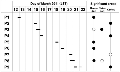
Fig. 2. Schematic diagrams of the transport routes analyzed in Nakajima et al. (2017) for plumes P1–P9 isolated in Tsuruta et al. (2014). Black arrows indicate the general movement trend for each plume. This figure is reprinted from fig. 15 in Nakajima et al. (2017). The letters, B, C, E, H, J, K1, K2, K3, 9, 12, and 15, indicate ¹³⁷Cs sample station locations identified in Nakajima et al. (2017) but these indications are not used in this study.

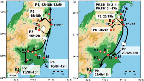
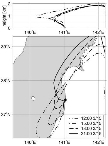
Nakajima et al. (2017) clearly identified these nine plumes, as shown in Fig. 2, and exhibited their model performance with hourly ¹³⁷Cs concentrations observed at 99 sample stations. However, we realized that several of the plume directions in Fig. 2 were inconsistent with the other forward trajectory model simulations. For example, Nakajima et al. (2017) claimed that plume P3 was transported toward the Nakadori region and crossed the Abukuma Mountains from south to north in the afternoon of 15 March 2011, Japanese Standard Time (JST); then, a part of plume P3 exhibited a northern detour from north to south in the late afternoon, as shown in Fig. 2a (geographical names are shown in Fig. 3). On the other hand, Kajino et al. (2016) calculated forward trajectories beginning at 12:00 JST, 15:00 JST, 18:00 JST, and 21:00 JST on 15 March 2011, from the FDNPP, which emitted the pollutant at 25-m height (Fig. 4). The forward trajectories described in Kajino et al. (2016) indicated that plume P3 rotated invariably clockwise and moved from south to north over the Abukuma Mountains and the Nakadori region in the late afternoon on 15 March 2011, JST. There is a discrepancy between observation-based analyses and forward trajectory analyses.

Fig. 3. Map of the area around the FDNPP. Closed diamonds indicate the ¹³⁷Cs sample stations in Tsuruta et al. (2014) and Oura et al. (2015).

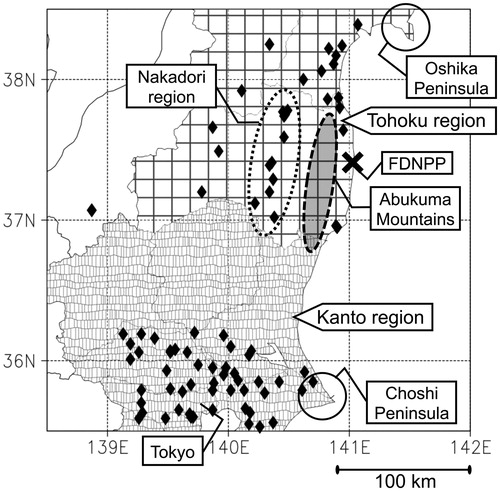
Fig. 4. Forward trajectories that began at 12:00 JST (dashed two-dot line), 15:00 JST (dashed-dotted line), 18:00 JST (dashed line), and 21:00 JST (solid line) on 15 March 2011 from the FDNPP at a height of 25 m (calculated by Kajino et al. 2016).

This discrepancy might be caused by dispersion model errors, meteorological analysis errors, or the vertical wind shear in the presence of the height difference between observations and the dominant stream of pollutant flows. In addition, neither the pollutant plumes in Fig. 2 nor the pollutant trajectories in Fig. 4 are quantitatively depicted regarding pollutant mass flows. We cannot determine which flow depiction is more plausible using only these simple figures. First, it is desirable that plumes of atmospheric pollutants should be identified and quantitatively determined when considering pollutant mass flows using dispersion models. This quantitative plume identification allows us to objectively validate the modeled dispersion performance and distinguish between dispersion and deposition errors.

In this study, we quantitatively depicted all of the plume streams (P1–P9) from Tsuruta et al. (2014) and Nakajima et al. (2017) using our ¹³⁷Cs dispersion model and attempted to determine the reasons for the abovementioned discrepancy. In this context, we took advantage of a mass flux analysis to quantify the pollutant flows. Mass flux is often used in fluid dynamics or dynamic meteorology (e.g. Iwasaki et al. 2014; Yano 2014); however, it has not been used as much in atmospheric chemistry or dispersion modeling, except for meridional transport analyses (e.g. Stohl et al. 2003; Belikov et al. 2013) or regional pollutant outflows (e.g. Bey et al. 2001). The concept of mass flux could be a robust alternative to traditional concepts using time-variable concentrations to assess horizontal pollutant flows. We attempt to exhibit the mass flux analysis as a model visualization method or a validation metric through the depiction of Fukushima ¹³⁷Cs plumes. In this analysis, we defined not only the single-layer mass flux but also the column-integrated mass flux to track pollutant mass flows that are vertically distributed. Details for the mass flux equations are described in Section 2, followed by a model description in Section 3. Then, a comparison of Fukushima ¹³⁷Cs plumes between our analysis results and those of Nakajima et al. (2017) is shown in Section 4, followed by concluding remarks in Section 5.

2. Mass flux and continuity equation

The mass flux $\mathbf{j}\mathrm{ }$is defined by the product of the mass concentration $\rho$ and the wind velocity $\mathbf{v}\equiv \mathrm{ }(u,\mathrm{ }v,\mathrm{ }w)$. $\mathbf{j}$ is represented as a mass per unit area per unit of time (e.g. kg m⁻² s⁻¹) or as the rate of mass flow per unit area (e.g. [kg s⁻¹] m⁻²), which perfectly corresponds with the momentum density or momentum per unit volume (e.g. [kg m s⁻¹] m⁻³). The mass flux indicates the extent that a pollutant is flowing over one’s head or how much a pollutant collides into one’s body per unit of time. Even if the mass concentration is known, the amount of total exposure cannot be estimated without the mass flux information. Furthermore, mass flux is a vector not a scalar (e.g. concentration); therefore, we can recognize the streams and directions of pollutant transport using the mass flux distribution.

In the atmosphere, the mass concentration and mass flux are governed by the continuity equation, which conserves the total mass of a pollutant as shown below (1) $$\begin{array}{c}\frac{\partial \rho }{\partial t}+\nabla \cdot \mathbf{j}=\frac{\partial \rho }{\partial t}+\nabla \cdot \rho \mathbf{v}=\frac{\partial \rho }{\partial t}+\frac{\partial \rho u}{\partial x}+\frac{\partial \rho v}{\partial y}+\frac{\partial \rho w}{\partial z}\\ =\frac{\partial \rho }{\partial t}+\nabla \cdot \rho {\mathbf{v}}_h+\frac{\partial \rho w}{\partial z}=\sigma ,\end{array}$$(1) where t represents time, ${\mathbf{v}}_h\equiv (u, v)$ represents the horizontal wind, and σ represents the generation of the pollutant per unit of volume and time. When σ > 0, σ is referred to as a source term. Conversely, when σ < 0, σ is referred to as a sink term. To achieve a vertically comprehensive assessment of mass flux in the atmosphere, we integrate Eq. (1)(1) $$\begin{array}{c}\frac{\partial \rho }{\partial t}+\nabla \cdot \mathbf{j}=\frac{\partial \rho }{\partial t}+\nabla \cdot \rho \mathbf{v}=\frac{\partial \rho }{\partial t}+\frac{\partial \rho u}{\partial x}+\frac{\partial \rho v}{\partial y}+\frac{\partial \rho w}{\partial z}\\ =\frac{\partial \rho }{\partial t}+\nabla \cdot \rho {\mathbf{v}}_h+\frac{\partial \rho w}{\partial z}=\sigma ,\end{array}$$(1) over a column from the surface to the top of the atmosphere; (2) $$\begin{array}{c}\underset{0}{\overset{\infty }{\int }}\left(\frac{\partial \rho }{\partial t}+\nabla \cdot \rho {\mathbf{v}}_h+\frac{\partial \rho w}{\partial z}\right)\mathrm{d}z=\underset{0}{\overset{\infty }{\int }}\frac{\partial \rho }{\partial t}\mathrm{d}z+\underset{0}{\overset{\infty }{\int }}\nabla \cdot \rho {\mathbf{v}}_h\mathrm{d}z+\underset{0}{\overset{\infty }{\int }}\frac{\partial \rho w}{\partial z}\mathrm{d}z\\ =\frac{\partial }{\partial t}\underset{0}{\overset{\infty }{\int }}\rho \mathrm{d}z+\nabla \cdot \underset{0}{\overset{\infty }{\int }}\rho {\mathbf{v}}_h\mathrm{d}z+{\left[\rho w\right]}_{z=0}^{z=\infty } (x, y, z, \text{and} t \text{are} \text{mutually} \text{independent})\\ =\frac{\partial }{\partial t}\underset{0}{\overset{\infty }{\int }}\rho \mathrm{d}z+\nabla \cdot {\mathbf{j}}_{\text{column}} (\because \rho (\infty )=w\left(0\right)=0)\\ =\underset{0}{\overset{\infty }{\int }}\sigma \mathrm{d}z={\sigma }_s,\end{array}$$(2) where σ_s represents deposition or emission at the surface, assuming that the pollutant is inert and is added/removed only at the surface. Here, we introduce the column integral of the horizontal mass flux, ${\int }_0^{\infty }\rho {\mathbf{v}}_h\mathrm{d}z\equiv {\mathbf{j}}_{\text{column}}$, which indicates the total mass flow per unit width integrated vertically from the surface to the top of the atmosphere (e.g. [kg s⁻¹] m⁻¹ = kg m⁻¹ s⁻¹). Conveniently, the time-integral of ${\mathbf{j}}_{\text{column}}$ illustrates the dominant stream of the pollutant two-dimensionally. Because the column integral of the vertical mass flux ${\int }_0^{\infty }\frac{\partial \rho w}{\partial z}\mathrm{d}z={\left[\rho w\right]}_{z=0}^{z=\infty }=0$ is negligible, the dominant stream can be calculated using only horizontal wind components and neglecting the vertical wind component, which is rarely obtained with high accuracy. This illustration is helpful when tracking pollutant plumes with a vertical structure.

Next, we integrate Eq. (2)(2) $$\begin{array}{c}\underset{0}{\overset{\infty }{\int }}\left(\frac{\partial \rho }{\partial t}+\nabla \cdot \rho {\mathbf{v}}_h+\frac{\partial \rho w}{\partial z}\right)\mathrm{d}z=\underset{0}{\overset{\infty }{\int }}\frac{\partial \rho }{\partial t}\mathrm{d}z+\underset{0}{\overset{\infty }{\int }}\nabla \cdot \rho {\mathbf{v}}_h\mathrm{d}z+\underset{0}{\overset{\infty }{\int }}\frac{\partial \rho w}{\partial z}\mathrm{d}z\\ =\frac{\partial }{\partial t}\underset{0}{\overset{\infty }{\int }}\rho \mathrm{d}z+\nabla \cdot \underset{0}{\overset{\infty }{\int }}\rho {\mathbf{v}}_h\mathrm{d}z+{\left[\rho w\right]}_{z=0}^{z=\infty } (x, y, z, \text{and} t \text{are} \text{mutually} \text{independent})\\ =\frac{\partial }{\partial t}\underset{0}{\overset{\infty }{\int }}\rho \mathrm{d}z+\nabla \cdot {\mathbf{j}}_{\text{column}} (\because \rho (\infty )=w\left(0\right)=0)\\ =\underset{0}{\overset{\infty }{\int }}\sigma \mathrm{d}z={\sigma }_s,\end{array}$$(2) over time for a typical plume situation, where the mass concentration is zero before a plume arrives and after it leaves. In this situation, $$\underset{0}{\overset{\infty }{\int }}\frac{\partial }{\partial t}\underset{0}{\overset{\infty }{\int }}\rho \mathrm{d}z\mathrm{d}t={\left[\underset{0}{\overset{\infty }{\int }}\rho \mathrm{d}z\right]}_{t=0}^{t=\infty }=0 (\because \rho \left(t=0\right)\equiv \rho \left(t=\infty \right)\equiv 0);$$ therefore, the integration of Eq. (2)(2) $$\begin{array}{c}\underset{0}{\overset{\infty }{\int }}\left(\frac{\partial \rho }{\partial t}+\nabla \cdot \rho {\mathbf{v}}_h+\frac{\partial \rho w}{\partial z}\right)\mathrm{d}z=\underset{0}{\overset{\infty }{\int }}\frac{\partial \rho }{\partial t}\mathrm{d}z+\underset{0}{\overset{\infty }{\int }}\nabla \cdot \rho {\mathbf{v}}_h\mathrm{d}z+\underset{0}{\overset{\infty }{\int }}\frac{\partial \rho w}{\partial z}\mathrm{d}z\\ =\frac{\partial }{\partial t}\underset{0}{\overset{\infty }{\int }}\rho \mathrm{d}z+\nabla \cdot \underset{0}{\overset{\infty }{\int }}\rho {\mathbf{v}}_h\mathrm{d}z+{\left[\rho w\right]}_{z=0}^{z=\infty } (x, y, z, \text{and} t \text{are} \text{mutually} \text{independent})\\ =\frac{\partial }{\partial t}\underset{0}{\overset{\infty }{\int }}\rho \mathrm{d}z+\nabla \cdot {\mathbf{j}}_{\text{column}} (\because \rho (\infty )=w\left(0\right)=0)\\ =\underset{0}{\overset{\infty }{\int }}\sigma \mathrm{d}z={\sigma }_s,\end{array}$$(2) over time is represented as (3) $$\underset{0}{\overset{\infty }{\int }}\nabla \cdot {\mathbf{j}}_{\text{column}}\mathrm{d}t=\underset{0}{\overset{\infty }{\int }}{\sigma }_s\mathrm{d}t,$$(3) 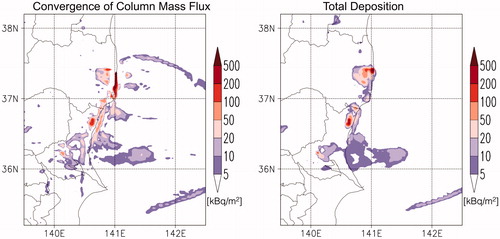which indicates that the time-integral for the divergence of the column integral in the horizontal mass flux equals the total emission or deposition per unit area (e.g. kg m⁻²). Actually, negative divergence (= convergence) and deposition are often very similar in ¹³⁷Cs plume model simulations. However, they are not exactly consistent because model simulations have numerical errors (mainly due to truncation processes) and assumption errors (e.g. non-zero background concentrations and finite limits of the model top height), as shown in Fig. 5. This figure was compiled using the ¹³⁷Cs dispersion model results detailed in the next section. The time-integrated period (21:00 JST on 20 March to 21:00 JST on 22 March 2011) was chosen to observe a noticeable example of wet deposition induced by widespread precipitation.

Fig. 5. Convergence (= negative divergence) of the column-integrated ¹³⁷Cs mass flux and the total deposition of ¹³⁷Cs values temporally integrated from 21:00 JST on March 20 to 21:00 JST on 22 March 2011 for the model simulation used in this study.

In addition, we can calculate a vertically mass-weighted mean wind, ${\mathbf{v}}_{\text{weighted}}$, by dividing the column integral of the horizontal mass flux by the total column mass (4) $${\mathbf{v}}_{\text{weighted}}\equiv \frac{{\mathbf{j}}_{\text{column}}}{\text{Total} \text{column} \text{mass}}=\underset{0}{\overset{\infty }{\int }}\rho {\mathbf{v}}_h\mathrm{d}z/\underset{0}{\overset{\infty }{\int }}\rho \mathrm{d}z,$$(4) which describes the wind velocity that forces the column-integrated mass from the ground surface to the top of the atmosphere.

3. Model description

In this study, the simulation of the Fukushima ¹³⁷Cs plume dispersion was performed by an offline Eulerian regional air quality model, which was originally developed by Kajino et al. (2012) for non-radioactive aerosol simulations. This dispersion model has been used for Fukushima nuclear pollutant simulation by Adachi et al. (2013), the Science Council of Japan (2014), Sekiyama et al. (2015, 2017), and Kajino et al. (2016). Radioactive ¹³⁷Cs nuclides were assumed to be contained in sulfate aerosol particles that were mixed with organic compounds, as described in detail by Sekiyama et al. (2015). We applied the ¹³⁷Cs emission scenario estimated by the Japan Atomic Energy Agency (Katata et al. 2015) to this simulation. Based on the time series of this emission scenario, ¹³⁷Cs-containing aerosol particles were injected into a grid cell above the FDNPP. The injection height was assigned based on the emission scenario, which varied temporally from 20 to 150 m.

This offline dispersion model was driven by meteorological grid point value (GPV) data calculated by the data assimilation system in Kunii (2014) and Sekiyama et al. (2015, 2017). The data assimilation system was composed of a non-hydrostatic regional weather prediction model (referred to as NHM; cf. Saito et al. 2006, 2007) and a local ensemble transform Kalman filter (LETKF; cf. Miyoshi and Aranami 2006). The NHM has been operationally used by the Japan Meteorological Agency (JMA) for daily national weather forecasts with a four-dimensional variation method; this weather forecast system is called JNoVA (cf. Honda et al. 2005). The LETKF was driven by 20 ensemble members at a 3-km horizontal resolution within a model domain over eastern Japan (215 × 259 grids; cf. fig. 2b of Sekiyama et al. 2015) and 60 vertical layers from the surface to 22 km above the surface. Details of the LETKF settings were described in Sekiyama et al. (2015, 2017). The boundary conditions for the model domain were provided by the JMA operational global analysis. Using the NHM and LETKF system (referred to as NHM-LETKF), we simultaneously assimilated the observations archived by the JNoVA system and the land surface wind observations collected by the JMA automated meteorological data acquisition system (AMeDAS), as described in Sekiyama et al. (2017). The AMeDAS is a land surface observation network that comprises ∼1300 stations throughout Japan, with an average interval of 17 km. The operational JNoVA dataset contains land surface pressure, satellite-observed sea surface winds, and observations from radiosondes, pilot balloons, wind profilers, aircrafts, ships and buoys.

The dispersion model shared the same model domain and horizontal resolution as those of the NHM-LETKF calculated meteorological GPV data, although the vertical resolution was converted from the original 60 layers (from the surface to 22 km) to 20 layers (from the surface to 10 km) to reduce the computational burden of calculations within the stratosphere. Meteorological GPV data were input into the dispersion model at 10-min intervals. In the dispersion model, the time step was set to 24 s using a linear interpolation of the meteorological GPV data. The model simulations were performed from 10 March to 31 March 2011.

4. Mass flux of Fukushima ¹³⁷Cs plumes

4.1. Insight into plume P3

First, we focus on Plume P3, which has a discrepancy between the observation-based analysis and the forward trajectory analysis, as mentioned in the Introduction. To track the dominant stream of the plume, the time-integral of the column-integrated mass flux ($\equiv {\int }_{t_1}^{t_2}{\mathbf{j}}_{\text{column}}\mathrm{d}t$; hereafter called the TC mass flux) of plume P3 is illustrated in Fig. 6a. The time-integration period was chosen to follow the classification of Tsuruta et al. (2014), shown in Fig. 1, and Nakajima et al. (2017), shown in Fig. 2, as much as possible. In this period (15:00 to 21:00 JST on 15 March 2011), the dominant stream (red or dark-red shading) flowed northwestward directly from the FDNPP and crossed the Abukuma Mountains toward the Nakadori region (Fig. 6a). Meanwhile, the widespread mass flux (which likely includes the residuals of plume P2 as shown in the panel P2 of Fig. 7) generally flowed northward or northeastward in the vicinity of the dominant stream of plume P3. This is consistent with the forward trajectory results of Kajino et al. (2016). The widespread and northeastward-directed TC mass flux occurred at an order of magnitude lower than that of the dominant stream directly emitted from the FDNPP. However, the arrow of plume P3 at 18:00 JST on 15 March from Nakajima et al. (2017), shown in Fig. 2 (also depicted as a large gray arrow in Fig. 6a), turns southwestward over the Nakadori region.

Fig. 6. Time-integrals from 15:00 to 21:00 JST on 15 March 2011 of (a) the column-integrated mass flux of plume P3 and (b) the horizontal mass flux of plume P3 at the ground surface. Color shading indicates the magnitude of the mass flux. Small arrowheads indicate the direction of the mass flux. A large gray arrow illustrates the depiction in Nakajima et al. (2017) for plume P3 at 18:00 JST on March 15, shown in Fig. 2. (c) Latitude-altitude cross-sections at 140.5°E for ¹³⁷Cs concentrations (gray shading), meridional winds (arrows), and potential temperature (θ; contours) at 17:00 JST on 15 March 2011. The cross-section is located at the green line in panel (b).

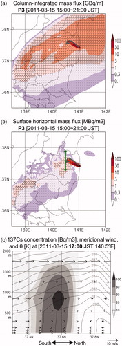
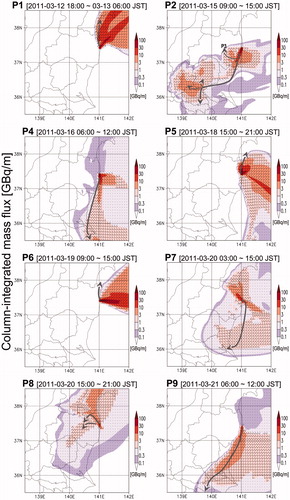
Fig. 7. Time-integrals of the column-integrated mass fluxes of plumes P1–P2 and P4–P9. Color shading indicates the magnitude of the mass flux. Small arrowheads indicate the direction of the mass flux. Gray arrows illustrate the depictions from Nakajima et al. (2017) for plumes P1–P2 and P4–P9, shown in Fig. 2. In figure P2, only part of the plume P3 arrows from Nakajima et al. (2017) in the vicinity of the FDNPP is illustrated.

Here, we pay attention not only to the TC mass flux but also to the horizontal mass flux at the ground surface (20 m) for plume P3 (Fig. 6b). The horizontal mass flux at the ground surface turned southwestward over the Nakadori region. This flow direction is consistent with that of Nakajima et al. (2017). The horizontal southwestward mass flux at the surface over the Nakadori region was a non-dominant stream that was approximately two orders of magnitude lower than that in the immediate vicinity of the FDNPP. The plume P3 direction shown by Nakajima et al. (2017) was analyzed only by means of the surface observations from Tsuruta et al. (2014). Therefore, these studies derived only the southwestward stream during this time slot. The two opposite stream directions are clearly depicted by the vertical cross-section of the pollutant concentration and the meridional wind (Fig. 6c). The maximum concentration core of plume P3 was located at a height of ∼900 m above the ground level (AGL), where southerly winds were occurring. In contrast, the surface wind direction was northerly beneath the plume core, although it was very weak. This indicates that a dominant stream of atmospheric pollutants cannot be determined using only ground surface observations.

4.2. Other plumes

Next, we surveyed each plume (P1–P2 and P4–P9) to analyze the TC mass flux direction and magnitude. Figure 7 shows the TC mass flux of Plumes P1–P2 and P4–P9 with plume pathway arrows from Nakajima et al. (2017) that are the same as those in Fig. 6a. The corresponding time-integration periods were chosen to follow the classification of Tsuruta et al. (2014), shown in Fig. 1, and Nakajima et al. (2017), shown in Fig. 2 (hereinafter called T&N), as much as possible.

The model-calculated TC mass flux of plume P1 flowed mainly northeastward over the Pacific Ocean and partly crossed the Oshika Peninsula located 120 km north-northeast of the FDNPP. The mass flux slightly flanked a coastal area north of the FDNPP, which was consistent with the plume depiction in T&N. The mainstream of Plume P1 was detected by dose rate monitoring posts at the Onagawa nuclear power plant in the Oshika Peninsula (the Tohoku Electric Power Company, http://www.tohoku-epco.co.jp/ICSFiles/afieldfile/2011/03/14/11031401_t1.pdf, in Japanese) during the P1 time slot (18:00 JST on 12 March to 06:00 JST on 13 March 2011). The monitoring post data indicated that the dose rates at the Oshika Peninsula slowly increased after 19:00 JST on 12 March, suddenly increased at 00:00 JST on 13 March, peaked at 02:00 JST on 13 March, and plateaued after 05:00 JST on 13 March; all of these stages were occurred during the P1 time slot.

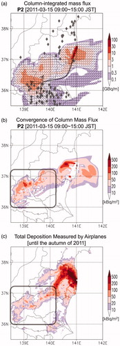
The model-calculated TC mass flux of plume P2 mainly flowed south-southwestward from the FDNPP, turned west, and spread over a large area in the Kanto region. This pathway was very consistent with those depicted in T&N. In addition, a northwestward flow was distinguished in the vicinity of the FDNPP, which was likely classified as part of plume P3 in T&N. Tsuruta et al. (2014) and Nakajima et al. (2017) proposed three terminal directions for plume P2: northeastward, northwestward, and southward over the Kanto region. The northeastward and northwestward flows were completely consistent with those illustrated by the TC mass flux. The dominant southward flows in T&N did not seem to be reproduced by the TC mass flux in Fig. 7. However, a southward (or southwestward) flow can be seen by plotting arrowheads for very small mass fluxes (Fig. 8a), although this flow was not dominant. Unfortunately, the observations in Tsuruta et al. (2014) and Oura et al. (2015) were not derived from the northern area of the Kanto region (shown in Fig. 8a). This biased distribution caused a bias in the plume analysis from T&N when the southward flow was supposed to be dominant. In practice, the northeastward/northwestward flows were presumably dominant and converged over the mountainous area of the northern Kanto region during this time period (shown by a gray rounded square in Fig. 8b). It is noted that the convergence (= deposition) was inconsistent or unnatural near the FDNPP because the time-integral length (= 6 h) was too short for the source area. The convergence area (shown by the gray rounded square) resembles the ¹³⁷Cs-polluted land surface over the mountainous area of the northern Kanto region in regard to shape and depth (Fig. 8c), which indicates that the convergence (= deposition) of Plume P2 is likely responsible for this land pollution. During this time period, it was drizzling (approximately <0.1 mm per 6 h) over this mountainous area in the model, which caused wet deposition.

Fig. 8. (a) Same as Fig. 7 for plume 2, but the plotted arrowheads include the direction of small mass fluxes <1 GBq m⁻¹. Gray diamonds indicate the ¹³⁷Cs sample stations from Tsuruta et al. (2014) and Oura et al. (2015). (b) Convergence of the column-integrated ¹³⁷Cs mass flux time-integrated during the period of plume 2 in the model simulation. (c) Total deposition measured by airplanes, which were recorded by the Japanese government (Torii et al. 2012). Note that this deposition represents all Cs-137 emissions and plumes until autumn of 2011.

Tsuruta et al. (2014) and Nakajima et al. (2017) inferred that plume P4 was transported by northerly winds over the ocean, which eventually reached the Choshi Peninsula. This depiction is clearly consistent with one of the two streams from the model-calculated TC mass flux during the P4 time slot. According to the TC mass flux depiction, the two streams were southward and eastward; the edge of the southward stream passed over the Choshi Peninsula, which is the easternmost area of the Kanto region.

Tsuruta et al. (2014) and Nakajima et al. (2017) reported that plumes P5 and P6 were short-duration events that occurred on 18 and 19 March, respectively, and both were observed over a limited area just north of the FDNPP. During these time slots, the plumes were mainly transported towards the Pacific Ocean, as shown by the model-calculated TC mass flux in Fig. 7. However, the peripheries of the plumes passed slightly over a coastal area north of the FDNPP. The ground surface observations in Tsuruta et al. (2014) likely detected these peripheries.

The model-calculated TC mass flux for plume P7 depicts a pathway characteristic of pollutant flows. The plume was transported over a long distance; first, it flowed southeastward with the offshore winds; second, it sharply turned clockwise toward the west over the ocean; then, it flowed onshore and landed over the Kanto region, as shown in Fig. 7. This pathway is obviously consistent with that referenced in T&N. Meanwhile, another northwestward flow was also depicted from the FDNPP, which was likely partially attributed to plume P8 because the P7 time slot overlapped with that of P8 (Fig. 1).

The depiction of plume P8 was somewhat similar to that of plume P3. The model-calculated TC mass flux indicated that a dominant stream flowed northwestward from the FDNPP and turned toward the northeast at ∼38°N. However, Tsuruta et al. (2014) and Nakajima et al. (2017) reported that plume P8 was transported northwestward from the FDNPP and redirected toward the south near the Nakadori region at the northern edge of the Abukuma Mountains (shown by gray arrows in Fig. 7). In the TC mass flux and T&N depictions, the plume rotates in the opposite direction. This inconsistency is discussed in the next section in detail.

Plume P9 followed a southern route and reached the Kanto region, which had sporadic rainfall during this time slot. This rainfall caused ¹³⁷Cs wet deposition in a wide range of areas in the Kanto region, which dispersed the plume (cf. Science Council of Japan 2014; Tsuruta et al. 2014; Sekiyama et al. 2015; Nakajima et al. 2017). The TC mass flux depicted the plume in a tongue shape that flowed southward from the FDNPP; then, it flowed to the northern part of the Kanto region and spread over southern parts of the Kanto region, as shown in Fig. 7. This pathway is precisely consistent with that of T&N, which is based on ground surface observations.

4.3. Inconsistency of plume P8

In the previous section, we encountered another inconsistent depiction between the TC mass flux and the T&N illustration for plume P8. The dominant stream of plume P8 flowed with the southerly winds throughout the entire period for the model-calculated TC mass flux; however, the stream exhibited an opposite rotation at the Abukuma Mountains for the T&N illustration. The discrepancy is likely to be caused by the difference in wind direction between the ground surface and the dominant layer of the mass flux, similar to that for plume P3. The horizontal mass flux at the ground surface (20 m), shown in Fig. 9a, clearly explains the two situations. The surface mass flux turned southwestward and propagated over the Nakadori region. Here, this flow direction was completely consistent with that of T&N based on ground surface observations. As shown in Fig. 9b, the high concentration core of plume P8 was distributed from the ground surface to ∼1000 m AGL at the beginning of the P8 time slot. At this time, the wind direction was northerly at <500 m AGL, and it was southerly at higher than 500 m AGL. This vertical wind shear caused an inconsistent depiction between the TC mass flux analysis and the surface observation analysis.

Fig. 9. (a) Time-integral of the horizontal mass flux at the ground surface for plume P8. The time-integrated period is consistent with that of plume P8 in Fig. 7. Color shading indicates the magnitude of the mass flux. Small arrowheads indicate the direction of the mass flux. Latitude-altitude cross-sections at 140.4°E for ¹³⁷Cs concentrations (gray shading), meridional wind (arrows), and potential temperature (θ; contours) are shown at (b) 15:00 JST on 20 March 2011 and (c) 17:00 JST on 20 March 2011. The cross-sections are located at the green line in panel (a).

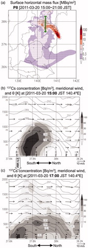
Then, the lower part of plume P8 was transported southward along the ground surface, while the upper part was transported northward along approximately isentropic surfaces. Consequently, the vertical cross-section shape of plume P8 arched over the ground in 2 h, as shown in Fig. 9c. Although the column-integrated mass flux is a useful tool to track atmospheric pollutants, a cross-check between the column-integrated and the ground surface mass fluxes is essential when the vertical wind shear is expected to be large.

5. Conclusions

We carried out a mass flux analysis for the Fukushima ¹³⁷Cs plumes by showing its usefulness and quantitative performance. The model-calculated TC mass flux was almost entirely consistent with the surface observations from Tsuruta et al. (2014) and Oura et al. (2015), although with some exceptions. However, these exceptions can be explained by the ground surface mass flux using together with the TC mass flux because the inconsistencies were only caused by the vertical wind shear between the ground surface and the dominant plume layer. The convergence of the TC mass flux was also able to explain the ¹³⁷Cs deposition distribution over northern Kanto region measured by airplanes.

The mass flux analysis clearly provided an overall illustration of dominant plume locations, directions, and depositions without developing movie/animation files. Unfortunately, such a useful mass flux analysis has rarely been used for dispersion simulations in atmospheric chemistry. The concept of the mass flux analysis can be further used as diagnostic or quantitative visualization tools because mass flux illustrations are a robust way for researchers to reduce high-dimensional model outputs into a lower-dimensional plot. It is inadequate to examine only a time series of concentrations at each observation point because such a conventional approach cannot validate the reproducibility of model-calculated mass flow balance. In contrast, the mass flux analysis can track the emission, advection, dispersion, and deposition of atmospheric constituents.

Acknowledgments

We thank Dr. Mizuo Kajino from the Meteorological Research Institute for providing us with his Lagrangian dispersion model. We also thank Prof. Teruyuki Nakajima from the Japan Aerospace Exploration Agency for kindly providing us with the figures in his paper.

Additional information

Funding

This work was supported by JSPS KAKENHI (under Grant JP16H02946, JP16H04051 and JP17K00533) and the Environment Research and Technology Development Fund (5-1605) at the Environmental Restoration and Conservation Agency (ERCA).

References

- Adachi, K., Kajino, M., Zaizen, Y. and Igarashi, Y. 2013. Emission of spherical cesium-bearing particles from an early stage of the Fukushima nuclear accident. Sci. Rep. 3, 2554. DOI:10.1038/srep02554.
- Belikov, D. A., Maksyutov, S., Krol, M., Fraser, A., Rigby, M. and co-authors. 2013. Off-line algorithm for calculation of vertical tracer transport in the troposphere due to deep convection. Atmos. Chem. Phys. 13, 1093–1114. DOI:10.5194/acp-13-1093-2013.
- Bey, I., Jacob, D. J., Logan, J. A. and Yantosca, R. M. 2001. Asian chemical outflow to the Pacific in spring: Origins, pathways, and budgets. J. Geophys. Res. 106, 23023–23097. DOI:10.1029/2001JD000806.
- Draxler, R., Arnold, D., Chino, M., Galmarini, S., Hort, M. and co-authors. 2015. World Meteorological Organization’s model simulations of the radionuclide dispersion and deposition from the Fukushima Daiichi nuclear power plant accident. J. Environ. Radioact. 139, 172–184. DOI:10.1016/j.jenvrad.2013.09.014.
- Honda, Y., Nishijima, M., Koizumi, K., Ohta, Y., Tamiya, K. and co-authors. 2005. A pre-operational variational data assimilation system for a non-hydrostatic model at the Japan Meteorological Agency: Formulation and preliminary results. Q. J. R Meteorol. Soc. 131, 3465–3475. DOI:10.1256/qj.05.132.
- Iwasaki, T., Shoji, T., Kanno, Y., Sawada, M., Ujiie, M. and co-author. 2014. Isentropic analysis of polar cold airmass streams in the northern hemispheric winter. J. Atmos. Sci. 71, 2230–2243. DOI:10.1175/JAS-D-13-058.1.
- Kajino, M., Inomata, Y., Sato, K., Ueda, H., Han, Z. and co-authors. 2012. Development of the RAQM2 aerosol chemical transport model and predictions of the Northeast Asian aerosol mass, size, chemistry, and mixing type. Atmos. Chem. Phys. 12, 11833–11856. DOI:10.5194/acp-12-11833-2012.
- Kajino, M., Ishizuka, M., Igarashi, Y., Kita, K., Yoshikawa, C. and co-authors. 2016. Long-term assessment of airborne radiocesium after the Fukushima nuclear accident: Re-suspension from bare soil and forest ecosystems. Atmos. Chem. Phys. 16, 13149–13172. DOI:10.5194/acp-16-13149-2016.
- Katata, G., Chino, M., Kobayashi, T., Terada, H., Ota, M. and co-authors. 2015. Detailed source term estimation of the atmospheric release for the Fukushima Daiichi Nuclear Power Station accident by coupling simulations of an atmospheric dispersion model with an improved deposition scheme and oceanic dispersion model. Atmos. Chem. Phys. 15, 1029–1070. DOI:10.5194/acp-15-1029-2015.
- Kunii, M. 2014. Mesoscale data assimilation for a local severe rainfall event with the NHM–LETKF system. Weather Forecasting 29, 1093–1105. DOI:10.1175/WAF-D-13-00032.1.
- Miyoshi, T. and Aranami, K. 2006. Applying a four-dimensional local ensemble transform Kalman filter (4D-LETKF) to the JMA nonhydrostatic model (NHM). SOLA 2, 128–131. DOI:10.2151/sola.2006-033.
- Nakajima, T., Misawa, S., Morino, Y., Tsuruta, H., Goto, D. and co-authors. 2017. Model depiction of the atmospheric flows of radioactive cesium emitted from the Fukushima Daiichi Nuclear Power Station accident. Prog. Earth Planet. Sci. 4, 2. DOI:10.1186/s40645-017-0117-x.
- Oura, Y., Ebihara, M., Tsuruta, H., Nakajima, T., Ohara, T. and co-authors. 2015. A database of hourly atmospheric concentrations of radiocesium (134Cs and 137Cs) in suspended particulate matter collected in March 2011 at 99 Air Pollution Monitoring Stations in Eastern Japan. J. Nucl. Radiochem. Sci. 15, 2_1–26. DOI:10.14494/jnrs.15.2_1.
- Saito, K., Fujita, T., Yamada, Y., Ishida, J-I., Kumagai, Y. and co-authors. 2006. The operational JMA nonhydrostatic mesoscale model. Mon. Weather Rev. 134, 1266–1298. DOI:10.1175/MWR3120.1.
- Saito, K., Ishida, J-I., Aranami, K., Hara, T., Segawa, T. and co-authors. 2007. Nonhydrostatic atmospheric models operational development at JMA. J. Meterolog. Soc. Jpn. 85B, 271–304. DOI:10.2151/jmsj.85B.271.
- Science Council of Japan. 2014. A review of the model comparison of transportation and deposition of radioactive materials released to the environment as a result of the Tokyo Electric Power Company’s Fukushima Daiichi Nuclear Power Plant accident. Report of Committee on Comprehensive Synthetic Engineering, Science Council of Japan. Available online at: http://www.jpgu.org/scj/report/20140902scj_report_e.pdf.
- Sekiyama, T. T., Kunii, M., Kajino, K. and Shimbori, T. 2015. Horizontal resolution dependence of atmospheric simulations of the fukushima nuclear accident using 15-km, 3-km, and 500-m grid models. J. Meteorol. Soc. Jpn. 93, 49–64. DOI:10.2151/jmsj.2015-002.
- Sekiyama, T. T., Kajino, M. and Kunii, M. 2017. The impact of surface wind data assimilation on the predictability of near-surface plume advection in the case of the Fukushima nuclear accident. J. Meteorol. Soc. Jpn. 95, 447–454. DOI:10.2151/jmsj.2017-025.
- Stohl, A., Wernli, H., James, P., Bourqui, M., Forster, C. and co-authors. 2003. A new perspective of stratosphere–troposphere exchange. Bull. Amer. Meteor. Soc. 84, 1565–1573. DOI:10.1175/BAMS-84-11-1565.
- Torii, T., Sanada, Y., Sugita, T., Kondo, A. and Shikaze, Y. 2012. Investigation of radionuclide distribution using aircraft for surrounding environmental survey from Fukushima Dai-ichi Nuclear Power Plant. JAEA-Technology 2012-036, Japan Atomic Energy Agency, 182 pp (in Japanese with English abstract)..
- Tsuruta, H., Oura, Y., Ebihara, M., Ohara, T. and Nakajima, T. 2014. First retrieval of hourly atmospheric radionuclides just after the Fukushima accident by analyzing filter-tapes of operational air pollution monitoring stations. Sci. Rep. 4, 6717. DOI:10.1038/srep06717.
- Yano, J.-I. 2014. Formulation structure of the mass-flux convection parameterization. Dyn. Atmos. Oceans 67, 1–28. DOI:10.1016/j.dynatmoce.2014.04.002.