Relationship between turbulent energy dissipation and gas transfer through the air–sea interface

Abstract

The nonlinear dependence of gas transfer velocity on wind speed typically results in the best fit of observational data; however, gas transfer velocity is dimensionally inconsistent with the nonlinear wind speeds. The objective of the current study was to show that, in the case of wind waves, gas transfer velocity with a consistent dimension should be determined by turbulent viscosity instead of by the viscosity of water when parameterised using the renewal model. Turbulent kinetic energy (TKE) near the air–sea interface is significantly intensified by breaking wind waves. By analyzing various models, we found that the TKE dissipation rate was explicitly linearly related to wind speed and dependent on wave age, with powers ranging from –2.36 to 4.0. Various models show that wave energy dissipation (WED) due to wind wave breaking explicitly increases with the cube of the wind speed and weakly depends on wave age. Assuming a balance between WED and total TKE dissipation in a constant dissipation layer, the depth of this layer was shown to be comparable to the wave height. Using the traditional renewal model with wind wave turbulent viscosity and TKE dissipation rate at the sea surface, we found that the gas transfer velocity was explicitly linearly related to wind speed in a dimensionally consistent manner, and depended simultaneously on the wave age and drag coefficient. These results are consistent with observational data obtained using the eddy correlation method. We emphasise that the linear dependence on wind speed is only valid when the wave age and drag coefficient are fixed; thus, this finding cannot be directly confirmed by currently available observational data due to a lack of wave state information.

Keywords:

• gas transfer velocity
• turbulence
• wind waves
• wave breaking

1. Introduction

For nonreactive gases such as CO₂, gas exchange through the air–sea interface can be modeled as a Fickian diffusive process and is therefore driven by two variables: the difference in gas partial pressure between air and water and the gas transfer velocity (k_L). The gas flux has been traditionally expressed as: (1) $$F=k_{L}s(p_{{\text{CO}}_{2w}}-p_{{\text{CO}}_{2a}})$$(1) where F is the gas flux across the air–sea interface, k_L is the gas transfer velocity, s is the solubility of CO₂, and p_CO2w and p_CO2a are the CO₂ partial pressures in water and air, respectively.

Because both atmospheric and aqueous CO₂ partial pressure can now be easily measured in the field (e.g. Vachon et al., 2010), the primary challenge in applying Equation (1)(1) $$F=k_{L}s(p_{{\text{CO}}_{2w}}-p_{{\text{CO}}_{2a}})$$(1) is to accurately estimate k_L, which is mainly related to turbulence in the water near the sea surface. Turbulence and k_L coupling was originally derived from surface renewal theory, based on the concept that turbulent eddies periodically bring fluid from the bulk to the surface (Danckwerts, 1951; Lamont and Scott, 1970). Considering the gas transfer related to turbulence and water viscosity, dimensional analysis can be used to express k_L as: (2) $$k_L=AS{c}^{-n}{(\epsilon \nu )}^{1/4}$$(2) where ε is the dissipation rate of turbulent kinetic energy (TKE) of water (m² s⁻³), ν is the kinematic viscosity of water, Sc = ν/D is the Schmidt number, D is the diffusion coefficient for the gas tracer, and A = 0.4 (Lamont and Scott, 1970) is a constant. The exponent n is 2/3 for a rigid surface and 1/2 for a free surface (Jähne et al., 1987). Therefore, n = 1/2 is usually adopted in the study of gas exchange through the air–sea interface. The remaining issue is how to estimate ε near the sea surface. One of the advantages of Equation (2)(2) $$k_L=AS{c}^{-n}{(\epsilon \nu )}^{1/4}$$(2) is the consistent dimensions of the two sides.

However, it is generally difficult to accurately measure TKE dissipation. In practical application, many studies have parameterised k_L in terms of wind speed (Liss and Merlivat, 1986; Wanninkhof, 1992; Weiss et al., 2007), where wind speed is used as an integrative proxy of turbulence. Thus, k_L is empirically expressed in the form: (3) $$k_L=aS{c}^{-1/2}{U}_{10}^b$$(3) where U₁₀ is the wind speed at a height of 10 m above the sea surface and the empirical constants a and b are determined by observational data. The exponent b usually ranges from 1.0 to 3.0 (Wanninkhof et al., 2009); this uncertainty shows that other processes and mechanisms also affect gas exchange. The nonlinear dependency of gas transfer velocity on wind speed is a result of the inconsistent dimensions of Equation (3)(3) $$k_L=aS{c}^{-1/2}{U}_{10}^b$$(3) .

In the case of wind waves, turbulence near the sea surface is governed by both wind speed and surface waves. The energy transferred from the wind field to waves is carried away by the group velocity of the waves; it is then transferred by nonlinear wave–wave interaction to other wavelengths and finally dissipated by steep waves into near-surface turbulence. Wind waves store a considerable amount of energy compared with that of the shear current. Even a weak breaking wave can contribute greatly to near-surface turbulence. Therefore, it is vital to investigate the relationship between wave energy dissipation (WED) and TKE dissipation rate to establish a reliable relationship between k_L and ε.

In the current study, we limited our analysis to wind waves with wave ages smaller than 1.4, such that wind energy is effectively input into waves. Our objective was to present a parameterisation of gas transfer velocity with a consistent dimension that can capture the observed nonlinearity of wind speed. We hypothesised that the viscosity of water should be replaced by turbulent viscosity, which depends on wind wave parameters when gas transfer velocity through the air–sea interface is parameterised by the renewal model. This study is organised as follows. In Section 2, we establish the relationship between ε and WED directly, by analyzing previous studies of turbulence and WED induced by wind waves. In Section 3, we show that wind wave turbulent viscosity should be used in the parameterisation of k_L. Finally, Section 4 presents our conclusions.

2. Relationship between TKE dissipation rate and WED

2.1. Models of TKE dissipation rate

For the case of wind waves, turbulence in the ocean surface layer is considered similar to that of waves found near rigid boundaries, in which shear production is approximately balanced by dissipation. Thus, ε can be scaled by the law of the wall: (4) $$\epsilon =\frac{u_{*w}^3}{\kappa z}$$(4) where κ = 0.40 is the von Kármán constant, z is the water depth, and u_*w is the friction velocity on the water side.

However, in the presence of breaking waves, field and laboratory measurements have shown that ε is significantly greater than expected from the law of the wall. According to turbulence observational data induced by wave breaking, Terray et al. (1996) proposed a profile model of the TKE dissipation rate near the sea surface; within a layer of depth z_b = 0.6H_s, ε is independent of depth and can be expressed as: (5) $${\epsilon }_{w0}=0.83\frac{{\alpha }_T{u}_{*w}^3}{H_s}$$(5) where H_s is the significant wave height, α_T = 0.5 (ρ_w/ρ_a)^1/2 β_*; β_* = c_p/u_* is wave age; c_p is the phase speed at the wind wave spectral peak; ρ_w and ρ_a are sea water and air densities, respectively; and ε_w0 denotes the TKE dissipation rate induced by the wind waves at the sea surface. Equation (5)(5) $${\epsilon }_{w0}=0.83\frac{{\alpha }_T{u}_{*w}^3}{H_s}$$(5) represents an important assumption made by Terray et al. (1996): that almost all of the wind energy input into waves is dissipated by the wave breaking process, and the remaining fraction is used to develop wind waves. This assumption has been confirmed in a recent study (Cavaleri et al., 2015). Invoking the wave growth relationship empirically proposed by Hanson and Phillips (1999), (6) $$H_s=0.18{\beta }^{1.61}{U}_{10}^2/g$$(6) where β = c_p/U₁₀ is the wave age, and g is the gravitational acceleration, Equation (5)(5) $${\epsilon }_{w0}=0.83\frac{{\alpha }_T{u}_{*w}^3}{H_s}$$(5) can be rewritten as: (7) $${\epsilon }_{w0}=2.7\times {10}^{-3}{\beta }^{-0.61}{C}_D^{}g{U}_{10}^{}$$(7) where C_D = u_*²/U₁₀² is defined as the drag coefficient. Equation (7)(7) $${\epsilon }_{w0}=2.7\times {10}^{-3}{\beta }^{-0.61}{C}_D^{}g{U}_{10}^{}$$(7) indicates that the TKE dissipation rate near the sea surface (ε_w0) is an explicitly linear function of wind speed, because C_D and β are implicitly related to wind speed. We limit our discussion here to wind waves, and consider swells with deflected, decreased, or no wind to be beyond the scope of this study. As wind waves develop, ε_w0 weakly decreases. It should be noted that Equation (7)(7) $${\epsilon }_{w0}=2.7\times {10}^{-3}{\beta }^{-0.61}{C}_D^{}g{U}_{10}^{}$$(7) is not a special case derived from observational data; many previous studies have suggested similar relationships.

Anis and Moum (1995) considered two wave turbulence interaction mechanisms for wind waves: one relying on TKE transport by orbital wave motions, and the other relying on the wave-induced shear stress that exists in a rotational wave field. Both mechanisms lead to an exponential relationship between z and ε_w, which can be expressed as: (8) $${\epsilon }_w=\frac{1}{8}{H}_s^{2}kg\hspace{0.17em}\text{sin}\hspace{0.17em}\varphi \frac{\partial U}{\partial z}{e}^{-2kz}$$(8) where k = 2π/L is the wave number, L is the wave length, U is the mean flow velocity in water, and ϕ is the phase shift from the quadrature of horizontal and vertical wave velocities. Stokes (1847) first theoretically derived drift induced by surface waves, which can be written as: (9) $$U_S\left(z\right)={\pi }^2{\delta }^{2}c\hspace{0.17em}\text{exp}(-2kz)$$(9) where c is the wave phase velocity, which can be regarded as c_p for wind waves, and δ = H_s/L is the wave steepness. According to the 3/2 power law proposed by Toba (1972) for wind waves, wave steepness can be written as: (10) $$\delta =0.135{\beta }^{-1/2}{C}_D^{1/4}$$(10)

Substituting Equation (10)(10) $$\delta =0.135{\beta }^{-1/2}{C}_D^{1/4}$$(10) into Equation (9)(9) $$U_S\left(z\right)={\pi }^2{\delta }^{2}c\hspace{0.17em}\text{exp}(-2kz)$$(9) , ε_w0 can be written as: (11) $${\epsilon }_{w0}=1.7\times {10}^{-3}{\beta }^{-1}{C}_D^{}g{U}_{10}$$(11) where sinϕ = 0.0523, following Anis and Moum (1995). Equation (11)(11) $${\epsilon }_{w0}=1.7\times {10}^{-3}{\beta }^{-1}{C}_D^{}g{U}_{10}$$(11) is consistent with Equation (7)(7) $${\epsilon }_{w0}=2.7\times {10}^{-3}{\beta }^{-0.61}{C}_D^{}g{U}_{10}^{}$$(7) , although they are derived from completely different contexts.

Alternatively, ε_w can be expressed as (Ardhuin and Jenkins, 2006): (12) $${\epsilon }_w=-u_{*w}^2\frac{\partial U_s}{\partial z}$$(12)

Substituting Equation (9)(9) $$U_S\left(z\right)={\pi }^2{\delta }^{2}c\hspace{0.17em}\text{exp}(-2kz)$$(9) into Equation (12)(12) $${\epsilon }_w=-u_{*w}^2\frac{\partial U_s}{\partial z}$$(12) and further invoking Equations (6)(6) $$H_s=0.18{\beta }^{1.61}{U}_{10}^2/g$$(6) and (10)(10) $$\delta =0.135{\beta }^{-1/2}{C}_D^{1/4}$$(10) , ε_w0 can be expressed as: (13) $${\epsilon }_{w0}=2.0\times {10}^{-3}{\beta }^{-2.11}{C}_D{}^{7/4}g{U}_{10}$$(13) where ε_w0 is again linearly related to U₁₀, and depends on β and C_D qualitatively, as in Equation (11)(11) $${\epsilon }_{w0}=1.7\times {10}^{-3}{\beta }^{-1}{C}_D^{}g{U}_{10}$$(11) .

According to the observational data of Anis and Moum (1995), Huang and Qiao (2010) modified Equation (12)(12) $${\epsilon }_w=-u_{*w}^2\frac{\partial U_s}{\partial z}$$(12) by introducing a dimensionless constant related to wave steepness. The resulting ε_w0 can be written as: (14) $${\epsilon }_{w0}=4.3\times {10}^{-3}{\beta }^{-2.36}{C}_D^{15/8}g{U}_{10}^{}$$(14)

The modification by Huang and Qiao (2010) alters the dependence on β and C_D quantitatively; however, their relationship remains qualitatively consistent with that in Equation (13)(13) $${\epsilon }_{w0}=2.0\times {10}^{-3}{\beta }^{-2.11}{C}_D{}^{7/4}g{U}_{10}$$(13) .

Benilov and Ly (2002) studied the general dynamic structure of the turbulent upper layer produced by wave breaking and turbulent diffusion of wave kinetic energy. Based on the similarity assumption leading to a universal relationship for wind waves, Kitaigorodskii (1998, 2001, 2011a) suggested that ε_w0 for these respective mechanisms can be described as: (15) $${\epsilon }_{w0}=1.2\times {10}^{-5}\beta g{U}_{10}$$(15) (16) $${\epsilon }_{w0}=1.12{\beta }^4{C}_D^{2}g{U}_{10}$$(16)

It is clear that Equations (15)(15) $${\epsilon }_{w0}=1.2\times {10}^{-5}\beta g{U}_{10}$$(15) and (16)(16) $${\epsilon }_{w0}=1.12{\beta }^4{C}_D^{2}g{U}_{10}$$(16) are explicitly linear functions of wind speed, as are Equations (7)(7) $${\epsilon }_{w0}=2.7\times {10}^{-3}{\beta }^{-0.61}{C}_D^{}g{U}_{10}^{}$$(7) , (13)(13) $${\epsilon }_{w0}=2.0\times {10}^{-3}{\beta }^{-2.11}{C}_D{}^{7/4}g{U}_{10}$$(13) , and (14)(14) $${\epsilon }_{w0}=4.3\times {10}^{-3}{\beta }^{-2.36}{C}_D^{15/8}g{U}_{10}^{}$$(14) ; the notable difference is the dependence of the former on wave age.

In addition to wave breaking, another contribution to the enhancement of TKE production is Langmuir circulation, which arises from the interaction of Stokes drift and wave-averaged currents driven by surface wind stress. Li and Garrett (1993) and Harcourt and D’Asaro (2008) suggested that Langmuir turbulence at the sea surface can be respectively estimated by: (17) $${\epsilon }_{w0}=1.42\times {10}^{-4}{C}_{D}g{U}_{10}$$(17) (18) $${\epsilon }_{w0}=1.79\times {10}^{-4}{\beta }^{-2}{C}_{D}g{U}_{10}$$(18)

Surprisingly, Equations (17)(17) $${\epsilon }_{w0}=1.42\times {10}^{-4}{C}_{D}g{U}_{10}$$(17) and (18)(18) $${\epsilon }_{w0}=1.79\times {10}^{-4}{\beta }^{-2}{C}_{D}g{U}_{10}$$(18) are also explicitly linear functions of wind speed and qualitatively consistent with parameterisations of ε_w0 induced by wave breaking.

Summarising the above analysis, ε_w0 can generally be expressed in the form: (19) $${\epsilon }_{w0}=a_1{\beta }^{b_1}{C}_D^{c_1}g{U}_{10}^{}.$$(19)

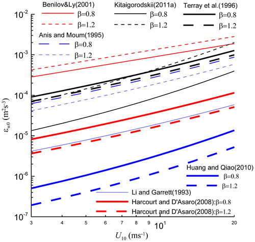
Table 1 lists the corresponding constants a₁, b₁, and c₁ for various models. Theoretical and observational studies have revealed that ε_w0 is an explicitly linear function of U₁₀ with significantly different dependence on β and C_D. The dependence on β varies qualitatively, with b₁ ranging from –2.36 to 4.0 (Table 1). This discrepancy remains to be further examined in future studies.

Table 1. Coefficients suggested by various studies for the TKE dissipation rate at the sea surface (Equation (28) in this study).

Authors	a1	b1	c1
Anis and Moum (1995)	1.7 × 10^–3	–1.0	1.0
Terray et al. (1996)	2.7 × 10^–3	–0.61	1.0
Benilov and Ly (2002)	1.2 × 10^–5	1.0	0.0
Huang and Qiao (2010)	4.3 × 10^–3	–2.36	1.875
Kitaigorodskii (2011a)	1.12	4.0	2.0
Li and Garrett (1993)	1.42 × 10^–4	0.0	1.0
Harcourt and D’Asaro (2008)	1.79 × 10^–4	–2.0	1.0

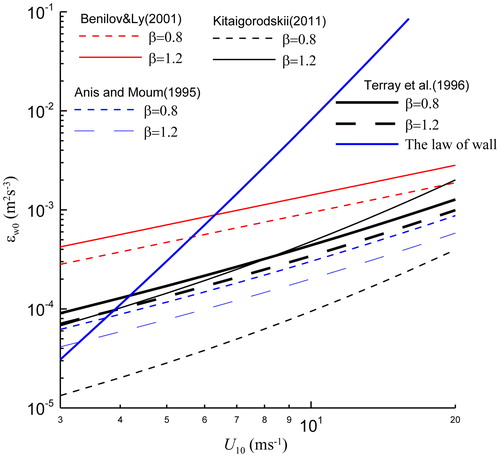
Figure 1 compares different models of ε_w0 using C_D = (0.8 + 0.065U₁₀) × 10⁻³ (Wu, 1980). The ε_w0 values derived from different models are qualitatively consistent; they differ significantly in magnitude due to variation in a₁, β, and C_D. The results of the models of Anis and Moum (1995) and Terray et al. (1996) were roughly consistent in magnitude and decrease with wave age. However, Kitaigorodskii’s (2011a) model produced significantly higher ε_w0 values as wave age increases; ε_w0 increased with wind speed due to its strong dependence on C_D. The model of Benilov and Ly (2002) provided the largest values among these models. It is reasonable that the models of Li and Garrett (1993) and Harcourt and D’Asaro (2008), which incorporated Langmuir turbulence, yielded significantly smaller ε_w0 values than those that considered wave breaking turbulence. However, it is surprising that the ε_w0 values of Huang and Qiao (2010) were significantly smaller than those of Li and Garrett (1993) and Harcourt and D’Asaro (2008).

Fig. 1. Comparison of various parameterisations of TKE dissipation rates at the sea surface (ε_w0) derived by analytical and empirical approaches.

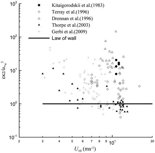
We collected observational ε_w0 data for the case of wind waves, including those collected by Kitaigorodskii et al. (1983), Terray et al. (1996), Drennan et al. (1996), Thorpe et al. (2003), and Gerbi et al. (2009). These data were obtained at depths ranging from 0.1 to 110 m, and wind speeds ranging from 3 to 15 m/s. The data used by Kitaigorodskii et al. (1983) and Terray et al. (1996) were obtained from the same fixed tower on Lake Ontario, which was installed in 12.5 m of water, 1.1 km from the western end of the lake. Thorpe et al. (2003) obtained their data from the coast of northwestern Scotland, between the islands of Mull and Colonsay and to the west of Colonsay, at water depths ranging from 40 to 110 m using an autonomous underwater vehicle (AUV). The AUV carried conductivity-temperature-depth sensors (CTDs), an acoustic Doppler current profiler (ADCP), a turbulence dissipation package, and forward- and starboard-pointing sidescan sonars. Gerbi et al. (2009) collected data at a tower located about 3 km south of Martha’s Vineyard, Massachusetts, in approximately 16 m of water. Velocity and waves were measured by Sontek 5-MHz acoustic Doppler velocimeters (ADVs). Figure 2 presents these observational data, normalised by the law of the wall, varying with wind speed. Most of the observational data were significantly greater than values predicted by the law of the wall, such that turbulence near the sea surface was greatly enhanced by wind waves and their breaking.

Fig. 2. Observational TKE dissipation rate data normalised by the law of the wall versus wind speed.

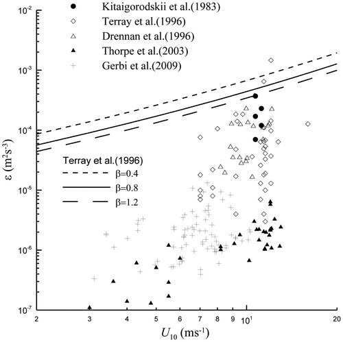
Figure 3 compares the results of Equation (7)(7) $${\epsilon }_{w0}=2.7\times {10}^{-3}{\beta }^{-0.61}{C}_D^{}g{U}_{10}^{}$$(7) with those of the observational data collected by Terray et al. (1996), who conducted more comprehensive experiments than others cited in the current study. Equation (7)(7) $${\epsilon }_{w0}=2.7\times {10}^{-3}{\beta }^{-0.61}{C}_D^{}g{U}_{10}^{}$$(7) serves as an upper bound for the observational data because it represents ε at the sea surface; however, it cannot be distinguished that observational values of ε linearly depend on U₁₀ because the data were measured at different depths (Fig. 3). Gerbi et al. (2009) conducted measurements at a sufficiently narrow range of depths (1.6–2.9 m) to assume a single depth; their data appear to show no significant increase with wind speed, in contrast to the observational data from other studies.

Fig. 3. Observational TKE dissipation rate data versus wind speed. The parameterisation by Terray et al. (1996) is shown for wave ages of 0.4, 0.8, and 1.2.

2.2. Wave energy dissipation of wind waves

Wave breaking is an important wave energy sink that governs the development of wind waves, when the wave age is smaller than 1.4. Hasselmann (1974) showed that the sink function of wave energy due to wave breaking is quasi-linear to the wave spectrum; this finding has been widely adopted in third-generation wave models. In contrast, based on an equilibrium wave spectrum argument, Phillips (1985) presented an analytical representation of the WED function that is proportional to the cube of the wave spectrum. Zhao and Toba (2001) estimated the total WED D_w (in W/m²) from the models of Phillips (1985) and Hasselmann (1974), respectively: (20) $$D_w=2.36\times {10}^{-3}{C}_D^{3/2}\hspace{0.17em}\text{ln}\left({\beta }_{*}\right){\rho }_w{U}_{10}^3$$(20) (21) $$D_w=2.21\times {10}^{-3}{C}_D^{3/2}{\rho }_w{U}_{10}^3.$$(21)

These two models are clearly generally consistent in their integral forms; both increase explicitly with the cubic wind speed. Based on observational data, Hanson and Phillips (1999) proposed a WED parameterisation, as: (22) $$D_w=4.28\times {10}^{-5}{U}_{10}^{3.74}.$$(22)

Thorpe (1993) conducted observations of wave-breaking frequency at a fixed positon for winds from 3 to 28 m/s, and his D_w can be expressed as: (23) $$D_w=9.375\times {10}^{-7}{\rho }_w{U}_{10}^3.$$(23)

By equating the wind input and WED, Hwang and Sletten (2008) derived D_w as: (24) $$D_w=\alpha {\rho }_w{U}_{10}^3,$$(24) where α = 2.33 × 10⁻⁴E _* β^−3.3, and E_* is nondimensional wave energy, defined as E_* = g²H_s²/(16U₁₀⁴). Many researchers have proposed that E_* can be expressed in the form E_* = a₂β^b2 (e.g., Toba, 1972, 1978; Mitsuyasu et al., 1980; Donelan et al., 1992; Glazman and Greysukh, 1993; Hanson and Phillips, 1999). Table 2 lists the empirical coefficients a₂, b₂, and the corresponding α. It is clear that D_w in Equation (24)(24) $$D_w=\alpha {\rho }_w{U}_{10}^3,$$(24) depends very weakly on wave age. Assuming that β = 0.9, the average α = 4.40 × 10⁻⁷, which is within the range of 4.31–5.48 × 10⁻⁷, as suggested by Hwang and Sletten (2008).

Table 2. Coefficients a₂ and b₂ for the nondimensional wave energy equation E_* = a₂β^b2 (see Section 2.2) and the corresponding α values.

Authors	a2 (×10^–3)	b2	α (×10^–7)
Toba (1972, 1978)	2.0	3.0	4.66β ^–0.3
Mitsuyasu et al. (1980)	1.7	3.0	3.96β ^–0.3
Donelan et al. (1992)	2.2	3.3	5.13
Glazman and Greysukh (1993)	1.4	3.23	3.26β^–0.07
Hanson and Phillips (1999)	2.0	3.22	4.66β^–0.08

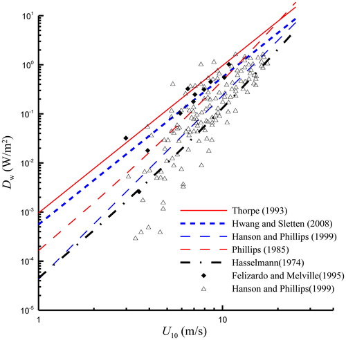
This analysis reveals that D_w is cubically related to wind speed, and very weakly dependent on wave age in the case of wind waves at β < 1.2 or β_* < 35. Thus, the energy of wind waves is mainly determined by wind speed. For the C_D value provided by Wu (1980) and β_* = 30, Fig. 4 compares the above WED models and observational data from Felizardo and Melville (1995) and Hanson and Phillips (1999). As shown in the figure, the models are consistent with observational data even in magnitude, especially at high wind speeds. Because C_D is a function of wind speed, the D_w formula proposed by Hasselmann (1974) and Phillips (1985) shows slightly more dependence on the wind speed than the cube of the wind speed. The dependence of D_W on wave age is very weak and can therefore be neglected.

Fig. 4. Comparisons of WED with wind speed. The models shown were proposed by Hasselmann (1974), Phillips (1985), Thorpe (1993), Hanson and Phillips (1999), and Hwang and Sletten (2008), using β_* = 30. Observational data from Felizardo and Melville (1995) and Hanson and Phillips (1999) are also plotted.

2.3. Relationship between wave and turbulence dissipation

In the case of wind waves, the turbulence near the sea surface is considered to be dominated by wave breaking. Assuming that turbulent dissipation locally balances the downward transport of enhanced surface turbulence produced by wave breaking, the total turbulence dissipation D_t (W/m²), vertically integrating ε (z) with depth, should be consistent with WED. Their relationship can be written as (Anis and Moum, 1995): (25) $$D_t={\rho }_w{\int }_0^{\infty }{\epsilon }_w\left(z\right)dz=D_w.$$(25)

To perform the integration, either continuous measurements of the ε profile or its parameterisation with depth are required. However, there is no general agreement on the parameterisation of ε.

In fact, as has been shown by considerable observational data, most of the turbulence induced by waves is limited to the layer near the sea surface, where a constant dissipation layer persists (Drennan et al., 1996; Terray et al., 1996; Kitaigorodskii, 2001; Young and Babanin, 2006). For simplification, we assume that D_t in the constant dissipation layer is equal to the WED, and that its depth is proportional to H_s. Therefore, D_t can be written as: (26) $$D_t\approx c_h{H}_s{\rho }_w{\epsilon }_{w0},$$(26) where c_h is a constant that can be determined by the equality of D_t to D_w. Notably, D_t ∝ U₁₀³, because ε_w0 ∝ U₁₀, H_s ∝ U₁₀², such that D_t and D_w have the same dimension and depend explicitly on the cube of the wind speed.

In our calculation, we used the D_w proposed by Hason and Phillips (1999) and Hwang and Sletten (2008) to equal D_t based on Equation (26)(26) $$D_t\approx c_h{H}_s{\rho }_w{\epsilon }_{w0},$$(26) . The best-fit results for c_h show that it is reasonable to assume that most turbulence induced by wave breaking is confined to a near-surface layer with thickness in the order of H_s (Table 3). In this manner, the energy estimated from wave models is comparable to that from TKE dissipation models, such that linear dependence of the TKE dissipation rate on wind speed is confirmed from the point of view of energy balance between turbulence and waves.

Table 3. Constant c_h, which is determined by equating D_t and D_w. HP99 and HS08 denote D_w as proposed by Hanson and Phillips (1999) and Hwang and Sletten (2008), respectively.

Authors	ch (HP99)	ch (HS08)
Anis and Moum (1995)	0.66	0.80
Terray et al. (1996)	0.42	0.56
Benilov and Ly (2002)	0.14	0.20
Kitaigorodskii (2011a)	0.26	0.32

3. Parameterisation of gas transfer velocity

3.1. Evaluation of the renewal model

As mentioned above, the determination of gas transfer is basically a problem of describing the structure of the turbulence in the subsurface layer of the ocean. In principle, k_L can be derived by Equation (2)(2) $$k_L=AS{c}^{-n}{(\epsilon \nu )}^{1/4}$$(2) if ε is determined. However, k_L from Equation (2)(2) $$k_L=AS{c}^{-n}{(\epsilon \nu )}^{1/4}$$(2) strongly depends on which ε depth is used.

Some studies have empirically demonstrated the universality of Equation (2)(2) $$k_L=AS{c}^{-n}{(\epsilon \nu )}^{1/4}$$(2) in different types of aquatic systems, in which ε was assumed to be independent of depth. Zappa et al. (2007) supported Equation (2)(2) $$k_L=AS{c}^{-n}{(\epsilon \nu )}^{1/4}$$(2) with A = 0.17–0.74 by field measurements in a range of systems including coastal ocean, a macro-tidal river estuary, a large tidal freshwater river, and an artificial ocean. Tokoro et al. (2008) measured gas transfer in coral reefs and estuaries using the floating chamber method. They found that Equation (2)(2) $$k_L=AS{c}^{-n}{(\epsilon \nu )}^{1/4}$$(2) with A = 0.13–0.22 agreed with their measurements. Vachon et al. (2010) performed a series of gas exchange measurements in 12 diverse aquatic systems ranging in size from less than 1 km² to more than 600 km². They found that their observational data were consistent with Equation (2)(2) $$k_L=AS{c}^{-n}{(\epsilon \nu )}^{1/4}$$(2) at A = 0.15–0.63.

Recently, Wang et al. (2015) conducted field measurements of near-surface turbulence with a novel floating particle image velocimetry system on Lake Michigan; k_L was derived from the simultaneously measured CO₂ flux by a floating gas chamber. To apply Equation (2)(2) $$k_L=AS{c}^{-n}{(\epsilon \nu )}^{1/4}$$(2) , they suggested that the coefficient A must be a function of ε, that is, A ∼ log ε, that was related to depth and dimensionally inconsistent. Under these conditions, the relation k_L ∼ (εν)^1/4 collapses.

In the case of wind waves, turbulence near the sea surface is dominated by wave breaking, in which ε_w0 varies linearly with wind speed, as in Equation (7)(7) $${\epsilon }_{w0}=2.7\times {10}^{-3}{\beta }^{-0.61}{C}_D^{}g{U}_{10}^{}$$(7) . Assuming that ν is constant and substituting Equation (7)(7) $${\epsilon }_{w0}=2.7\times {10}^{-3}{\beta }^{-0.61}{C}_D^{}g{U}_{10}^{}$$(7) into Equation (2)(2) $$k_L=AS{c}^{-n}{(\epsilon \nu )}^{1/4}$$(2) , we obtain: (27) $$k_L\propto U_{10}^{1/4}.$$(27)

It is clear that such a weak dependence of k_L on U₁₀ is never observed in any stage of wind wave development. The only quantity subsumed by ε that implicitly depends on wind speed is C_D. However, many studies have shown that C_D is generally linearly related to wind speed, and cannot significantly alter the dependence of k_L on wind speed indicated in Equation (27)(27) $$k_L\propto U_{10}^{1/4}.$$(27) .

Alternatively, Lorke and Peeters (2006) argued that Equation (4)(4) $$\epsilon =\frac{u_{*w}^3}{\kappa z}$$(4) could successfully be applied to estimate k_L in a manner comparable to common empirical parameterisations through Equation (2)(2) $$k_L=AS{c}^{-n}{(\epsilon \nu )}^{1/4}$$(2) , by adopting the Kolmogorov length scale. By using the Kolmogorov length scale in Equation (4)(4) $$\epsilon =\frac{u_{*w}^3}{\kappa z}$$(4) , they suggested that the TKE dissipation rate at the sea surface (ε₀) can be expressed as: (28) $${\epsilon }_0=0.384C_D^2{U}_{10}^4.$$(28)

From Equation (28)(28) $${\epsilon }_0=0.384C_D^2{U}_{10}^4.$$(28) , ε₀ increases with the fourth power of the wind speed. Considering the dependence of C_D on wind speed, Equation (28)(28) $${\epsilon }_0=0.384C_D^2{U}_{10}^4.$$(28) shows an extraordinary dependence on wind speed that has never been observed in any measurement data. As shown in Fig. 5, ε₀ obtained by Equation (28)(28) $${\epsilon }_0=0.384C_D^2{U}_{10}^4.$$(28) is significantly greater than that produced by any other model, especially at high wind speeds. Substituting Equation (28)(28) $${\epsilon }_0=0.384C_D^2{U}_{10}^4.$$(28) into Equation (2)(2) $$k_L=AS{c}^{-n}{(\epsilon \nu )}^{1/4}$$(2) , Lorke and Peeters (2006) obtained the gas transfer velocity k_L (Sc = 660): (29) $$k_L=1.56\times {10}^{-4}{C}_D^{1/2}{U}_{10}.$$(29)

Fig. 5. Comparison of TKE dissipation rates obtained using the law of the wall (Equation 28) with those obtained for breaking waves.

The advantage of Equation (29)(29) $$k_L=1.56\times {10}^{-4}{C}_D^{1/2}{U}_{10}.$$(29) is dimensional consistency. Previously developed empirical parameterisations of k_L involving the square or cube of the wind speed have inconsistent dimensions, even though they best fit their observational data. However, many studies have shown that the law of the wall cannot be applied in the presence of wind waves, as discussed in Section 2. Therefore, although k_L derived from Equation (29)(29) $$k_L=1.56\times {10}^{-4}{C}_D^{1/2}{U}_{10}.$$(29) is comparable to observed gas transfer velocity values, its essential premise is doubtful.

3.2. Parameterisation by the renewal model

As explained in the above discussion, previous studies that claimed to support the renewal model, Equation (2)(2) $$k_L=AS{c}^{-n}{(\epsilon \nu )}^{1/4}$$(2) , faced a challenge in determining how to select a value of ε that strongly depends on depth while k_L has a unique value that is independent of depth. In this context, Equation (2)(2) $$k_L=AS{c}^{-n}{(\epsilon \nu )}^{1/4}$$(2) is a poor relationship from which to estimate k_L, unless ε can be found to be independent of depth.

We suggest that the depth dependence of ε can be avoided via an equivalent to WED. As wind waves develop, the viscous sublayer of the ocean is completely destroyed by the vigorous turbulence induced by wave breaking. Under these conditions, instead of molecular viscosity (ν), turbulent viscosity (ν_t) should be used in Equation (2)(2) $$k_L=AS{c}^{-n}{(\epsilon \nu )}^{1/4}$$(2) . Therefore, Equation (2)(2) $$k_L=AS{c}^{-n}{(\epsilon \nu )}^{1/4}$$(2) should be modified as: (30) $$k_L=AS{c}^{-n}{\left({\epsilon }_{w0}{\nu }_t\right)}^{1/4},$$(30) where ν_t is directly related to wind waves.

Many studies have parameterised ν_t in the presence of wind waves. In their comprehensive book about ocean waves, Wen and Yu (1985) introduced two methods that can be applied to derive ν_t near the sea surface in terms of wave parameters. Both are based on the von Kármán mixing length theory and the horizontal velocity of water particle induced by water waves, that is, ν_t = 2κ²π⁻²H_sc_p and ν_t = κ²(36)⁻²gH_s²/c_p. Their difference lies in the horizontal velocity of a water particle being estimated by the small amplitude or cycloid wave theory. Invoking Equation (6)(6) $$H_s=0.18{\beta }^{1.61}{U}_{10}^2/g$$(6) and the definition of wave age, ν_t can be respectively expressed as: (31) $${\nu }_t=5.8\times {10}^{-3}{\beta }^{2.61}{U}_{10}^3/g$$(31) (32) $${\nu }_t=1.44\times {10}^{-4}{\beta }^{2.22}{U}_{10}^3/g.$$(32)

In both expressions, the parameter increases with wind speed cubically, and both have roughly the same dependence on wave age. A similar result was also provided by Kitaigorodskii (1998), under the assumption that the amplitude of the grid oscillation in grid-generated turbulence can be compared with the amplitude of breaking wind waves in the upper ocean.

Based on the models of ε_w0 presented in Section 2 and Equation (31)(31) $${\nu }_t=5.8\times {10}^{-3}{\beta }^{2.61}{U}_{10}^3/g$$(31) or Equation (32)(32) $${\nu }_t=1.44\times {10}^{-4}{\beta }^{2.22}{U}_{10}^3/g.$$(32) , k_L can be derived from Equation (30)(30) $$k_L=AS{c}^{-n}{\left({\epsilon }_{w0}{\nu }_t\right)}^{1/4},$$(30) . For example, using Equations (32)(32) $${\nu }_t=1.44\times {10}^{-4}{\beta }^{2.22}{U}_{10}^3/g.$$(32) and (7)(7) $${\epsilon }_{w0}=2.7\times {10}^{-3}{\beta }^{-0.61}{C}_D^{}g{U}_{10}^{}$$(7) , k_L can be expressed as: (33) $$k_L=9.73\times {10}^{-4}A{\beta }^{0.4}{C}_D^{1/4}{U}_{10},$$(33) where Sc = 660. In this manner, k_L is explicitly linearly related to wind speed and increases with wave age. One of the advantages of Equation (33)(33) $$k_L=9.73\times {10}^{-4}A{\beta }^{0.4}{C}_D^{1/4}{U}_{10},$$(33) is dimensional consistency.

It should be pointed out that k_L is not exactly explicitly linearly dependent on wind speed. In addition to wind speed, Equation (33)(33) $$k_L=9.73\times {10}^{-4}A{\beta }^{0.4}{C}_D^{1/4}{U}_{10},$$(33) also depends on wave age or the drag coefficient, which are functions of wind speed. When only these parameters are fixed, our results show perfectly linear dependence on wind speed. Current observational data including various wave states cannot directly support this linear dependence using the best-fit method. For this reason, empirical formulas for gas transfer velocity are generally not linear functions of wind speed.

3.3. Discussion

From physical principles, many previous studies have determined that gas transfer velocity is explicitly linearly dependent on wind speed. Csanady (1990) indicated that k_L can be written as: (34) $$k_L=7.07\times {10}^{-4}{C}_D^{1/2}{U}_{10}.$$(34)

Although Equations (33)(33) $$k_L=9.73\times {10}^{-4}A{\beta }^{0.4}{C}_D^{1/4}{U}_{10},$$(33) and (34)(34) $$k_L=7.07\times {10}^{-4}{C}_D^{1/2}{U}_{10}.$$(34) are obtained from very different contexts, they are almost completely consistent, with a slight difference in their dependence on wave age. Soloviev (2007) suggested that ε can be written as the sum of convective and shear forces and wave breaking, and that k_L can be simplified as: (35) $$k_L\approx 8.4\times {10}^{-5}{C}_{\mathrm{D}}^{1/2}{U}_{10}$$(35)

Kitaigorodskii (2011b) suggested that k_L increases as wind waves grow, and can be written as: (36) $$k_L=3.1\times {10}^{-4}\beta C_{\mathrm{D}}^{1/2}{U}_{10}.$$(36)

We emphasise that k_L is explicitly linearly dependent on wind speed only because it also depends on C_D and β.

In practice, two types of observations have been used to obtain gas transfer velocities: tracer and eddy correlation methods. The tracer method usually involves a long averaging time, for example, several hours or days. The eddy correlation method is a well-established surface flux technique that focuses on short time scales, that is, 10–60 min. It is clear that our results are better suited to instantaneous data obtained through the eddy correlation method. Therefore, we use such data for comparison with the model results.

Taking A = 0.2 as an average value for field measurements obtained in previous studies (e.g. Zappa et al., 2007; Tokoro et al., 2008; Vachon et al., 2010), Fig. 6 shows observational data and parameterisations of k_L by substitution in various models of ε_w0 into Equation (30)(30) $$k_L=AS{c}^{-n}{\left({\epsilon }_{w0}{\nu }_t\right)}^{1/4},$$(30) ; the Equation (36)(36) $$k_L=3.1\times {10}^{-4}\beta C_{\mathrm{D}}^{1/2}{U}_{10}.$$(36) model is plotted for comparison. Due to the dependence of ν_t on wave age in Equations (31)(31) $${\nu }_t=5.8\times {10}^{-3}{\beta }^{2.61}{U}_{10}^3/g$$(31) and (32)(32) $${\nu }_t=1.44\times {10}^{-4}{\beta }^{2.22}{U}_{10}^3/g.$$(32) , nearly all of the k_L values derived from Equation (30)(30) $$k_L=AS{c}^{-n}{\left({\epsilon }_{w0}{\nu }_t\right)}^{1/4},$$(30) increase with wave age. Because a fixed wave age is not realistic under varying wind speeds, we assume that wave age increases linearly from 0.1 to 1.4 as wind speed increases.

Fig. 6. Relationship between wind speed and gas transfer velocities obtained from various models including those derived from Equation (30) with A = 0.2 and wave age changing from 0.1 to 1.4 with wind speed, and various parameterisations of the TKE dissipation rate, and model from Kitaigorodskii (2011b). Observational data obtained by the eddy correlation method are added for comparison (regression curve: thin solid black line).

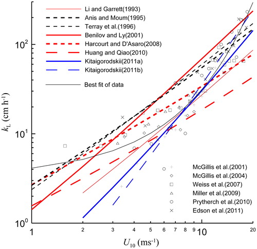
Figure 6 shows that the parameters determined using Equation (30)(30) $$k_L=AS{c}^{-n}{\left({\epsilon }_{w0}{\nu }_t\right)}^{1/4},$$(30) are comparable to the observations, even when ε is derived from Langmuir turbulence, as in Li and Garrett (1993) and Harcourt and D’Asaro (2008). In this context, it is clear that the dependence of gas transfer velocity on wind speed is nonlinear, and consistent with the observational data. Additionally, combining four tracer measurements in the North Sea, Nightingale et al. (2000) show in their fig. 13 that k_L increases with H_s, which implies an increase with wave age. In terms of the wind–sea Reynolds number, Zhao et al. (2003; Zhao and Xie, 2010) also implicitly indicated that k_L increases with wave age.

Another important parameter affecting gas transfer is wave steepness (δ), which strongly controls wave breaking. In general, wave steepness increases with decreasing wave age, and their relationship can be expressed as δ = β⁻²(gH_s/2πU₁₀²), utilising the deep water dispersion relationship. However, compared to wave age, wave steepness information is more difficult to obtain because wave length cannot be measured directly. Therefore, wave steepness is usually replaced by wave age.

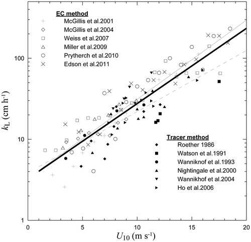
Figure 7 compares observational data from previous studies obtained by eddy correlation and tracer methods. The eddy correlation results appear to be greater than the tracer results as a whole, although their differences are insignificant. According to the least squares method, k_L is more likely an exponential function of wind speed than a linear or square function. Figure 7 plots the regression results of all data, eddy correlation data, and tracer data in thick solid, thin solid, and dashed lines, respectively. The thick solid line (all data) is expressed as: (37) $$k_{\mathrm{L}}=3.251\hspace{0.17em}\text{exp}\left(0.214U_{10}\right),$$(37) where k_L is in cm/h and U₁₀ in m/s. It is clear that current observational data cannot describe k_L robustly due to a lack of information about wave age and wave steepness, which is important for the parameterisation of gas transfer.

Fig. 7. Comparison of observational data obtained by eddy correlation and tracer methods. Thick solid line, think solid line, and dashed solid line indicate regression results for all data (3.251 exp(0.214U₁₀)), eddy correlation data (3.294 exp(0.225U₁₀)), and tracer method data (3.112 exp(0.174U₁₀)), respectively.

4. Conclusion

We analysed various models of the TKE dissipation rate and WED. In the case of wind waves, ε_w0 for either wave breaking or Langmuir circulation can be expressed as an explicitly linear function of wind speed, and its dependence on wave age is very scattered and inconsistent. The explicitly linear dependence on wind speed cannot be directly confirmed by observation due to a lack of information about wave states and sufficient data at the same water depth. WED explicitly increases in wind waves as the cube of the wind speed, and weakly depends on wave age. Assuming that turbulence induced by wave breaking is limited to a constant dissipation layer near the sea surface, in which the turbulent energy is equal to the wave energy, we conclude that the thickness of this constant dissipation layer is one order greater than the wave height, which is consistent with the observations.

In the case of wind waves, molecular viscosity in the traditional renewal model should be replaced by the turbulent viscosity related to wind waves. Thus, the gas transfer velocity is explicitly linearly dependent on wind speed and increases with wave age and the drag coefficient. When the scale coefficient A = 0.2, the result is comparable to observational data under the assumption that wave age varies with wind speed. This new model has dimensional consistency and can capture the observed nonlinear dependence on wind speed with varying wave age. We emphasise that the linear wind dependence of k_L is valid only when wave age is fixed, and cannot be confirmed by current observational data because they are collected during various wave states.

Acknowledgments

We thank the researchers who obtained and published the data adopted in this study as well as their respective funding organisations. The observational data read from these published papers are available from Dongliang Zhao via e-mail: [email protected].

Disclosure statement

No potential conflict of interest was reported by the authors.

Additional information

Funding

This work was supported by the Public Science and Technology Research Funds for Ocean Projects (201505007), National Natural Science Foundation of China (NSFC, 41876010, 41276015, 41076007), and the Joint Project for the National Oceanographic Center by the NSFC and the Shandong Government (U1406402).

References

- Anis, A. and Moum, J. N. 1995. Surface wave-turbulence interactions: scaling ε (z) near the sea surface. J. Phys. Oceanogr. 25, 1222–1227.
- Ardhuin, F. and Jenkins, A. D. 2006. On the interaction of surface wave and upper ocean turbulence. J. Phys. Oceanogr. 36, 551–557. DOI:10.1175/JPO2862.1.
- Benilov, A. Yu. and Ly, L. N. 2002. Modelling of surface waves breaking effects in the ocean upper layer. Math. Comput. Modell. 35, 191–213. DOI:10.1016/S0895-7177(01)00159-5.
- Cavaleri, L., Bertotti, L. and Bidlot, J.-R. 2015. Waving in the rain. J. Geophys. Res. Oceans. 120, 3248–3260. DOI:10.1002/2014JC010348. DOI:10.1002/2014JC010348.
- Csanady, G. T. 1990. The role of breaking wavelets in air-sea gas transfer. J. Geophys. Res. 95, 749–759.
- Danckwerts, P. V. 1951. Significance of liquid–film coefficients in gas absorption. Ind. Eng. Chem. 43, 1460–1467. DOI:10.1021/ie50498a055.
- Donelan, M. A., Skafel, M. G., Graber, H., Liu, P., Schwab, D. and Venkatesh, S. 1992. On the growth rate of wind–generated waves. Atmos. Ocean. 30, 457–478.
- Drennan, W. M., Donelan, M. A., Terray, E. A. and Katsaros, K. B. 1996. Oceanic turbulence dissipation measurements in SWADE. J. Phys. Oceanogr. 26, 808–815. DOI:10.1175/1520-0485(1996)026<0808:OTDMIS>2.0.CO;2.
- Felizardo, F. and Melville, W. K. 1995. Correlations between ambient noise and the ocean surface wave field. J. Phys. Oceanogr. 25, 513–532. DOI:10.1175/1520-0485(1995)025<0513:CBANAT>2.0.CO;2.
- Gerbi, G. P., Trowbridge, J. H., Terray, E. A., Plueddemann, A. J., Kukulka, T. and co-authors. 2009. Observations of turbulence in the ocean surface boundary layer: energetics and transport. J. Phys. Oceanogr. 39, 1077–1096. DOI:10.1175/2008JPO4044.1.
- Glazman, R. E., and Greysukh, A. 1993. Satellite altimeter measurements of surface wind. J. Geophys. Res. 98, 2475–2483.
- Hanson, J. L. and Phillips, O. M. 1999. Wind sea growth and dissipation in the open ocean. J. Phys. Oceanogr. 29, 1633–1648. DOI:10.1175/1520-0485(1999)029<1633:WSGADI>2.0.CO;2.
- Harcourt, R. R. and D’Asaro, E. A. 2008. Large-eddy simulation of Langmuir turbulence in pure wind seas. J. Phys. Oceanogr. 38, 1542–1562. DOI:10.1175/2007JPO3842.1.
- Hasselmann, K. 1974. On the spectral dissipation of ocean waves due to whitecapping. Bound.Layer Meteor. 126, 507–127.
- Huang, C. J. and Qiao, F. 2010. Wave-turbulence interaction and its induced mixing in the upper ocean. J. Geophys. Res. 115, C04026. DOI:10.1029/2009JC005853.
- Hwang, P. A. and Sletten, M. A. 2008. Energy dissipation of wind-generated waves and whitecap coverage. J. Geophys. Res. 113, C02012, DOI:10.1029/2007JC004277.
- Jähne, B., Munnich, K. O., Bosinger, R., Dutzi, A., Huber, W. and Libner, P. 1987. On the parameters influencing air–water gas exchange. J. Geophys. Res. 92, 1937–1949.
- Kitaigorodskii, S. A. 1998. The dissipation subrange in wind wave spectra. Geophysica. 34, 179–207.
- Kitaigorodskii, S. A. 2001. On the influence of wind wave breaking on the structure of the subsurface oceanic turbulence. Izv. Atmosph. Ocean. Phys. 37, 566–576.
- Kitaigorodskii, S. A. 2011a. The influence of wind wave breaking on the dissipation of the turbulent kinetic energy in the upper ocean and its dependence on the stage of wind-wave development. In: Gas Transfer at Water Surfaces 2010 (eds. S. Komori, W. McGillis and R. Kurose), Kyoto University Press, Kyoto, pp. 29–37.
- Kitaigorodskii, S. A. 2011b. The calculation of the gas transfer between the ocean and atmosphere. In: Gas Transfer at Water Surfaces 2010, (eds. S. Komori, W. McGillis and R. Kurose, Kyoto University Press, Kyoto. pp. 13–28.
- Kitaigorodskii, S. A., Donelan, M. A., Lumley, J. L. and Terray, E. A. 1983. Wave–turbulence interaction in the upper ocean. Part II: Statistical characteristics of wave and turbulence components of the random velocity field in the marine surface layer. J. Phys. Oceanogr. 13, 1988–1999. DOI:10.1175/1520-0485(1983)013<1988:WTIITU>2.0.CO;2.
- Lamont, J. C. and Scott, D. S. 1970. An eddy cell model of mass transfer into the surface of a turbulent liquid. AIChE J. 16, 513–519. DOI:10.1002/aic.690160403.
- Li, M. and Garrett, C. 1993. Cell merging and the jet/downwelling ratio in Langmuir circulation. J. Mar. Res. 51, 737–769. DOI:10.1357/0022240933223945.
- Liss, P. S. and Merlivat, L. 1986. Air–sea gas exchange rates: Introduction and synthesis. In: The Role of Air–Sea Exchange in Geochemical Cycling (eds. P. Buat-Menard), D. Reidel, Norwell, MA, pp. 113–129.
- Lorke, A. and Peeters, F. 2006. Toward a unified scaling relation for interfacial fluxes. J. Phys. Oceanogr. 36, 955–961. DOI:10.1175/JPO2903.1.
- Mitsuyasu, H., Tasai, F., Suhara, T., Misuno, S., Ohkuso, M., Honda, T., and Rikiishi, K.. 1980. Observations of the power spectrum of ocean waves using a cloverleaf buoy. J. Phys. Oceanogr. 10, 286–296.
- Nightingale, P. D., Malin, G., Law, C. S., Watson, A. J., Liss, P. S., and co-authors. 2000. In situ evaluation of air–sea gas exchange parameterizations using novel conservative and volatile tracers. Global Biogeochem. Cycles. 14, 373–387.
- Phillips, O. M. 1985. Spectral and statistical properties of the equilibrium range in wind generated gravity waves. J. Fluid Mech. 156, 505–531. DOI:10.1017/S0022112085002221.
- Soloviev, A. V. 2007. Coupled renewal model of ocean viscous sublayer thermal skin effect and interfacial gas transfer velocity. J. Mar. Syst. 66, 19–27. DOI:10.1016/j.jmarsys.2006.03.024.
- Stokes, G. G. 1847. On the theory of oscillatory waves. Trans. Cambridge Philos. Soc. 8, 441–455.
- Terray, E. A., Donelan, M. A., Agrawal, Y. C., Drennan, W. M., Kahma, K. K., and co-authors. 1996. Estimates of kinetic energy dissipation under breaking waves. J. Phys. Oceanogr. 26, 792–807. DOI:10.1175/1520-0485(1996)026<0792:EOKEDU>2.0.CO;2.
- Thorpe, S. A. 1993. Energy loss by breaking waves. J. Phys. Oceanogr. 23, 2498–2502. DOI:10.1175/1520-0485(1993)023<2498:ELBBW>2.0.CO;2.
- Thorpe, S. A., Osborn, T. R., Jackson, J. F. E., Hall, A. J. and Lueck, R. G. 2003. Measurements of turbulence in the upper–ocean mixing layer using Autosub. J. Phys. Oceanogr. 33, 122–145. DOI:10.1175/1520-0485(2003)033<0122:MOTITU>2.0.CO;2.
- Toba, Y. 1972. Local balance in the air–sea boundary processes. I. On the growth processes. J. Oceanogr. Soc. Jpn. 28, 109–120. DOI:10.1007/BF02109772.
- Toba, Y. 1978. Stochastic form of the growth of wind waves in a single-parameter representation with physical implications. J. Phys. Oceanogr. 8, 494–507.
- Tokoro, T., H., Kayanne, A., Watanabe, K., Nadaoka, H., Tamura, K. and co-authors. 2008. High gas-transfer velocity in coastal regions with high energy-dissipation rates. J. Geophys. Res. 113, C11006. DOI:10.1029/2007JC004528.
- Vachon, D., Prairie, Y. T. and Cole, J. J. 2010. The relationship between near-surface turbulence and gas transfer velocity in freshwater systems and its implications for floating chamber measurements of gas exchange. Limnol. Oceanogr. 55, 1723–1732. DOI:10.4319/lo.2010.55.4.1723.
- Wang, B., Liao, Q., Fillingham, J. H. and Bootsma, H. A. 2015. On the coefficients of small eddy and surface divergence models for the air–water gas transfer velocity. J. Geophys. Res. Oceans. 120, 2129–2146. DOI:10.1002/2014JC010253.
- Wanninkhof, R. 1992. Relationship between gas exchange and wind speed over the ocean. J. Geophys. Res. 97, 7373–7381.
- Wanninkhof, R., Asher, W. E., Ho, D. T., Sweeney, C. S. and McGillis, W. R. 2009. Advances in quantifying air-sea gas exchange and environmental forcing. Ann. Rev. Mar. Sci. 1, 213–244. DOI:10.1146/annurev.marine.010908.163742.
- Weiss, A., Kuss, J., Peters, G. and Schneider, B. 2007. Evaluating transfer velocity–wind speed relationship using a long-term series of direct eddy correlation CO2 flux measurements. J. Mar. Syst. 66, 130–139. DOI:10.1016/j.jmarsys.2006.04.011.
- Wen, S. and Yu, Z. 1985. Ocean-Wave Theory and Computational Principle (in Chinese). Science Press, Beijing.
- Wu, J. 1980. Wind stress coefficients over sea surface near neutral conditions: a revisit. J. Phys. Oceanogr. 10, 727–740. DOI:10.1175/1520-0485(1980)010<0727:WSCOSS>2.0.CO;2.
- Young, I. R. and Babanin, A. V. 2006. Spectral distribution of energy dissipation of wind-generated waves due to dominant wave breaking. J. Phys. Oceanogr. 36, 376–394. DOI:10.1175/JPO2859.1.
- Zappa, C. J., McGillis, W. R., Raymond, P. A., Edson, J. B., Hintsa, E. J., and co-authors. 2007. Environmental turbulent mixing controls on air–water gas exchange in marine and aquatic systems. Geophys. Res. Lett. 34, L10601. DOI:10.1029/2006GL028790.
- Zhao, D. and Toba, Y. 2001. Dependence of whitecap coverage on wind and wind-wave properties. J. Oceanogr. 57, 603–616. DOI:10.1023/A:1021215904955.
- Zhao, D. and Xie, L. 2010. A practical bi-parameter formula of gas transfer velocity depending on wave states. J. Oceanogr. 66, 663–671. DOI:10.1007/s10872-010-0054-4.
- Zhao, D., Toba, Y., Suzuki, Y. and Komori, S. 2003. Effect of wind waves on air–sea gas exchange: proposal of an overall CO2 transfer velocity formula as a function of breaking-wave parameter. Tellus. 55, 478–487.