Predicting atmospheric particle formation days by Bayesian classification of the time series features

Abstract

Atmospheric new-particle formation (NPF) is an important source of climatically relevant atmospheric aerosol particles. NPF can be directly observed by monitoring the time-evolution of ambient aerosol particle size distributions. From the measured distribution data, it is relatively straightforward to determine whether NPF took place or not on a given day. Due to the noisiness of the real-world ambient data, currently the most reliable way to classify measurement days into NPF event/non-event days is a manual visualization method. However, manual labor, with long multi-year time series, is extremely time-consuming and human subjectivity poses challenges for comparing the results of different data sets. These complications call for an automated classification process. This article presents a Bayesian neural network (BNN) classifier to classify event/non-event days of NPF using a manually generated database at the SMEAR II station in Hyytiälä, Finland. For the classification, a set of informative features are extracted exploiting the properties of multi-modal log normal distribution fitted to the aerosol particle concentration database and the properties of the time series representation of the data at different scales. The proposed method has a classification accuracy of 84.2 % for determining event/non-event days. In particular, the BNN method successfully predicts all event days when the growth and formation rate can be determined with a good confidence level (often labeled as class Ia days). Most misclassified days (with an accuracy of 75 %) are the event days of class II, where the determination of growth and formation rate are much more uncertain. Nevertheless, the results reported in this article using the new machine learning-based approach points towards the potential of these methods and suggest further exploration in this direction.

Keywords:

• atmospheric aerosol particles
• new-particle formation
• machine learning
• Bayesian neural networks

1. Introduction

The Earth’s atmosphere, while providing shelter and comfort for its inhabitants, also hosts a multitude of interesting and interconnected physical processes. Among these the phenomenon of atmospheric new-particle formation (NPF) has attracted growing scientific attention during the last few decades (Nieminen et al., 2014). By providing an initial surface for a significant fraction of cloud condensation nuclei, the tiny secondary atmospheric aerosol particles are crucial players in cloud and climate processes (Bianchi et al., 2016). Thus, atmospheric scientists are interested in understanding how various processes modify the properties of aerosol particles and especially how, why and when these particles form.

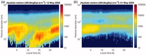
The most straightforward way to investigate NPF in depth is to directly measure these events in the ambient atmosphere. Typically, this is done by observing the time-evolution of the particle size distributions. Figure 1 shows example of both an event day (Fig. 1a: clear NPF and growth to large sizes) and a non-event day (Fig. 1b: no clear NPF).

Fig. 1. Examples of an event (a) and a non-event (b) day at Hyytiälä, Finland, in May 2005. The x-axis shows one 24-h time period whereas the y-axis shows the range of particle size diameters (from 3 to 1000 nm). The color scale indicates particle concentration (cm^{– 3}). In (a) one can clearly see aerosol particles forming around noon and then growing into larger sizes. This data was accessed via Smart-SMEAR (Junninen et al., 2009).

The current procedure for generating the database of aerosol formation days is based on the visualization method, proposed by Dal Maso et al., (2005). Although the visualization method and the event classes, it introduced have been received very well by the atmospheric community, at the same time, it is acknowledged that the utilization of the method requires significant manual labor. Furthermore, as the classification in the end is determined by human judgement, inconsistencies may arise between different datasets due to unavoidable human subjectivity. Thus, robust automated procedures for data analysis are called for (Kulmala et al., 2012).

Although modern data science provides new techniques to tackle large data sets. Neural networks have been one of the most successful machine learning (ML) methods which have been applied widely in many applications (Hagan et al., 2014). In particular, modern day deep neural network (DNN) learning methods are tailored to find the essence of large datasets, therefore, they might also help in dealing with the atmospheric data. But one of the major drawbacks of deep learning approaches is that huge amount of data and computational resources are required for training such models.

The second most common issue that arises in DNN training is over-fitting, i.e. if the number of model parameters is too large, the model tends to overfit the training data and its ability to generalise on the test dataset is restricted. Hence, we propose to use a Bayesian neural network (BNN) classifier which is known method not only with good generalisation capability but also relatively less computationally expensive then the DNN (Szegedy et al., 2015). This method utilizes the representative features extracted from time series data to automatize the classification process of atmospheric aerosol particle formation days.

2. Atmospheric data

In this work, we utilize the aerosol particle size distribution data gathered at the SMEAR II station in Hyytiälä, Finland.

2.1. Sampling site: SMEAR II Hyytiälä, Finland

The SMEAR II station is located in Hyytiälä forestry field station in southern Finland (${61}^{°} 51\prime$N, ${24}^{°} 17\prime$E, 181 m above sea level), about 220 km northwest of Helsinki. This station lies between two big cities, Tampere and Jyväskylä. It is surrounded by homogeneous Scots-pine-dominated forests. Hyytiälä forest is classified as a rural background site considering the levels of air pollutants, shown by e.g. submicron aerosol number size distributions (Asmi et al., 2011; Nieminen et al., 2014). The SMEAR II has been established for multidisciplinary research, including atmospheric sciences, soil chemistry and forest ecology. A detailed description of the continuous measurements performed at this station can be found in Kulmala et al., (2001) and Hari and Kulmala (2005).

In particular, aerosol particle number concentration size distributions are measured with a twin-Differential Mobility Particle Sizer (DMPS) system with condensation particle counters (Aalto et al., 2001). The system comprises two separate DMPS instruments, the first instrument measures the particle sizes between 3 and 50 nm and another DMPS measures the larger particles. When SMEAR II was first operated, the measured particle size distributions ranged from 3 to 500 nm until December 2004. After that, it was extended to cover the size range from 3 to 1000 nm (Nieminen et al., 2014). In the last few years, the size of the smallest particles that can be detected has decreased from 3 nm to around one nanometer (Kulmala et al., 2012). Nevertheless, in this study, we only utilize particle sizes ranging from 3 to 1000 nm due to the availability of the classification database needed for the neural network training and validation.

2.2. Database: classification of aerosol particle formation days

In order to perform supervised learning, an input–output database is required to train classification or regression models (Bishop, 2006). Here, we use a variety of features extracted from the aerosol particle concentration database for the training of the proposed method. Please see Section 3 for further details related to feature extraction and the classification methodology. For determining the class information, i.e. event/non-event days, we use a classification database created by the atmospheric scientists at the University of Helsinki during the years 1996–2014. The database has been constructed by a visual inspection method (Dal Maso et al., 2005) of the continuously measured aerosol size distributions over a size range of 3–1000 nm at SMEAR II Hyytiälä. The method classifies the days into three main categories, which are event, non-event and undefined days.

An event day occurs when there is a growing new mode in the nucleation size range prevailing over several hours, whereas a non-event day is assumed when the day is clear of all traces of particle formation. A day is defined to be an undefined day when it cannot be unambiguously classified as either an event or a non-event day. To avoid any bias in the training of the neural network, we exclude the undefined days in this study.

The NPF event days can be further divided into class I and class II based on their confidence level. Class I is assumed when the growth and formation rate can be determined with a good confidence level, whilst class II occurs when the derivation of these parameters is not possible or there is a doubt in the accuracy of the results. Class I can be still further divided into sub-classes Ia and Ib. Class Ia is assumed when the day shows a very clear and strong particle formation event, with very little or no pre-existing particles obscuring the newly formed mode, whereas class Ib contains the remaining class I events. An example of four different types of NPF days is shown in Fig. 2. In this study, we attempt to teach a neural network to classify the days only into event and non-event days. The sub-class classification of NPF days provides useful information while analysing the result of the classification performance.

Fig. 2. Four different types of NPF days, classified based on the method proposed by Dal Maso et al. (2005). The x-axis shows the 24-h time period, whereas y-axis represents the range of particle diameters (from 3 to 1000 nm). The color indicates the particle concentration (cm^-3).

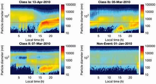
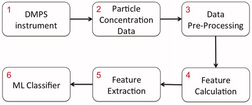
Fig. 3. Schematic diagram of the ML methodology for classifying aerosol particle formation days.

3. Machine learning method

Figure 3 illustrates the proposed ML classification strategy. Aerosol particle concentration data (the second box) obtained from the DMPS instruments (the first box) is used in this analysis. These data need to be pre-processed first (the third box) before it is fed into the ML model. This section describes the methodology for data pre-processing and obtaining the relevant features. The BNN classifier used in this study is briefly introduced in the final subsection.

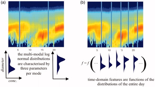
Fig. 4. From the concentration data, two types of features are calculated to be used in the learning and validating of the neural network. At each instance of time, the ambient aerosol particle distribution can be presented as a multi-modal log normal distribution, characterized by three parameters per mode (see panel (a)). The set of these fitted parameters are used as the first type of features given to the neural network. The ambient particle distribution evolves throughout the day and this change is manifested in the parameters of the log normal distributions. A set of time-domain quantities calculated over the entire measurement day (excluding nighttime) are given to the neural network as second type of features (see panel (b) and Table 1).

3.1. Data pre-processing and feature extraction

In the data pre-processing step, we remove outlier data points, which are typically due to sensor faults or extreme conditions. Undefined days are also excluded to reduce the uncertainty in training dataset because this class cannot be unambiguously classified as either an event or non-event day, hence may give rise to human associated bias.

In the feature calculation step, the pre-processed data are then used to calculate representative features which can be used in the actual ML process. Here, we consider the following two types of quantities:

3.1.1. Mmulti-modal log normal distribution function

The first set of features consists of the properties of a multi-modal log normal distribution function. Most aerosol particle size distributions can be fitted with this distribution function (Whitby, 1978). The multi-modal log normal distribution function, f, can be expressed mathematically by (1) $$f\left(D_p,{\overline{D}}_{pg,i},N_i,{\sigma }_{g,i}\right)=\sum _{i=1}^n\frac{N_i}{\sqrt{2\pi }\hspace{0.17em}\text{log}\left({\sigma }_{g,i}\right)}\times \hspace{0.17em}\text{exp}\hspace{0.17em}\left[-\frac{{\left[\text{log}\left(D_p\right)-\hspace{0.17em}\text{log}\left({\overline{D}}_{pg,i}\right)\right]}^2}{2{\hspace{0.17em}\text{log}\hspace{0.17em}}^2\left({\sigma }_{g,i}\right)}\right]$$(1) where D_p and n are the diameter of an aerosol particle and the number of individual log-normal modes that characterize the particle number size distribution, respectively. This distribution function also comprises three tuned parameters. The parameters N_i, ${\sigma }_{g,i}^2$ and $D_{pg,i}$ represent the mode concentration, geometric variance and geometric mean diameter, respectively. In this case, these parameters are fitted using an automatic algorithm developed by Hussein et al., (2005). The fitting is done at each instance of time and the fitted parameters are considered as the properties of the multi-modal log normal distributions, which will then be used as the first type of ML feature.

3.1.2. Time-domain features

The second set of ML features are the time domain properties of aerosol particle concentrations, such as mean, standard deviation, kurtosis and skewness. These features are adopted from time-domain signal processing techniques described in Howard (1994) and Allen and Mills (2004). These features utilize the amplitude vs. time characteristic of aerosol particles concentration. In other words, we calculate all features mentioned in Table 1 for every type of particle size per day. This results in a single value per particle size termed as a feature of the time series. Once all the features for all types of particle size are calculated they are then fed to the BNN model as inputs for the training purpose. Table 1 shows all the calculated time-domain features used in this study. In this case, x(i) is the number of concentration at time i for every particle size distribution.

Table 1. Time-domain feature representations used in this study. The notation of x(i) and N denote the signal x(i) at time i and the number of data points, respectively. In this case, the signal is equivalent with the concentration level of every particle size distribution.

Time-domain features	Formula
Mean ($\overline{x}$)	$\frac{1}{N}{\sum }_{i=1}^N(x(i))$
Variance	$\frac{1}{N}{\sum }_{i=1}^N{(x(i)-\overline{x})}^2$
Standard Deviation	$\sqrt{\frac{1}{N}{\sum }_{i=1}^N{(x(i)-\overline{x})}^2}$
RMS value (RMS)	$\sqrt{\frac{1}{N}{\sum }_{i=1}^N|x(i){|}^2}$
Peak value (PV)	$\frac{1}{2}(\text{max}(x(t))-\text{min}(x(t)))$
Kurtosis	$\frac{\frac{1}{N}{\sum }_{i=1}^N{(x(i)-\overline{x})}^4}{{(\frac{1}{N}{\sum }_{i=1}^N{(x(i)-\overline{x})}^2)}^2}$
Crest factor	$\frac{\text{PV}}{\text{RMS}}$
Skewness	$\frac{\frac{1}{N}{\sum }_{i=1}^N{(x(i)-\overline{x})}^3}{{(\sqrt{\frac{1}{N}{\sum }_{i=1}^N{(x(i)-\overline{x})}^2})}^3}$
Clearance factor	$\frac{\text{PV}}{\frac{1}{N}{({\sum }_{i=1}^N\sqrt{|x(i)|})}^2}$
Impulse factor	$\frac{\text{PV}}{\frac{1}{N}{\sum }_{i=1}^N|x(i)|}$
Shape factor	$\frac{\text{RMS}}{\frac{1}{N}{\sum }_{i=1}^N|x(i)|}$
K-Factor	$\text{PV}·\text{RMS}$

These two types of ML features are illustrated in Fig. 4. The parameters of a multi-modal log normal distribution can be seen as features calculated from the y-axis of the NPF ‘banana plot’, whereas the time-domain features are calculated from the x-axis. This way the ML procedure should be able to take into account both the instantaneous shape of the aerosol particle distribution and the evolution of the distribution. This strategy enables us to construct an information-rich feature set to distinguish between the event and the non-event days.

Fig. 5. The cumulative sum of eigenvalues of the data in Principal Component (PC) space. In order to retain 99 per cent of original data information, we need to select only the first 69 PCs from almost 400 calculated features.

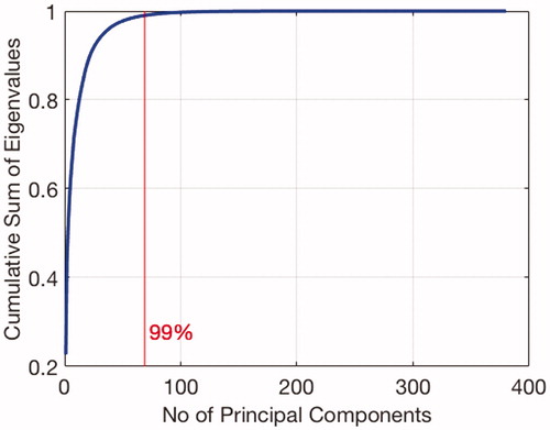
The combination of the first and second feature sets results in a large data dimension, which may lead to the ‘curse of dimensionality’: the proposed algorithm may perform poorly with very high-dimensional data (Bishop, 2006). Therefore, as illustrated in the fifth box in Fig. 3, a set of dominant features are extracted which is then finally used to train the ML model. Principal component analysis (PCA) (Pearson, 1901) is a popular technique to perform dimensionality reduction for large data sets (Lu, Plataniotis, and Venetsanopoulos 2011). In this case, we use PCA to project all of the obtained features onto principal components (PCs) space. Then, we select only the directions with highest variance PCs for the input of ML model. Figure 5 illustrates the cumulative sum of eigenvalues of the data in the PC space. It can be seen that there are almost 400 calculated features which can be reduced to be only 69 PCs as ML features by retaining 99 % information from original calculated features. Finally, the selected PCs are fed into the selected ML method (the last box in Fig. 3), that is a BNN classifier. Nevertheless, other ML approaches may also be adopted and implemented using this general strategy. BNN classifier will be introduced briefly in the following subsection.

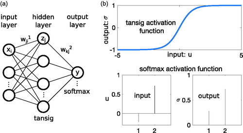
Fig. 6. Schematic representation of a BNN with one hidden layer (a) and the used activation functions (b).

3.2. Bayesian neural network

We use a BNN (Bishop, 2006) to model the unknown relationship, $\mathbf{y}=f(\mathbf{x})$, between the features x and their corresponding event/non-event days output y. Unlike standard neural networks (Lippmann, 1987), BNN uses Bayesian inference in optimizing the network weights. It adds a regularization term to the network performance function. This steers the training towards simpler neural networks, thus reducing the risk of over-fitting.

Figure 6a shows a schematic representation of the neural network. The input layer consists of an M-dimensional array $\mathbf{x}=\left\{x_1,x_2,\dots ,x_M\right\}$, containing the number of selected features M (in our case M = 69). In this case, the output y is just a binary number (e.g. zero and one), representing event/non-event days. The jth neuron in the Lth layer computes its output $z_j^L$ as follows: (2) $$z_j^L=\sigma \left(\sum _i{w}_{ji}^L{x}_i+b_j^L\right)$$(2) where $w_{ji}^L$ is the weight of connection between the computing neuron and its ith input in the preceding layer, and $b_j^L$ is an additional bias parameter.

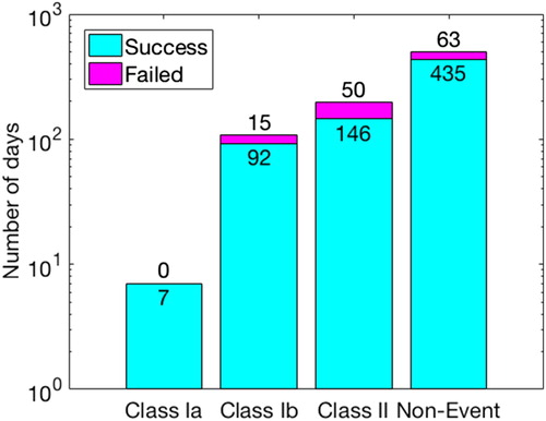
Fig. 7. The bar chart of the successful and unsuccessful number of predicted days.

The symbol $\sigma ()$ represents an activation function. In this case, the used activation functions for the hidden layer and the output layer are hyperbolic tangent sigmoid (tansig) and softmax basis functions, respectively. They are expressed mathematically as follows: (3) $$\sigma \left(u\right)=\text{tansig}\left(u\right) \hspace{1em}=\frac{2}{1+{\hspace{0.17em}\text{exp}\hspace{0.17em}}^{-2u}}-1$$(3) (4) $$\sigma \left(u_p\right)=\text{softmax}\left(u_p\right)=\frac{{\hspace{0.17em}\text{exp}\hspace{0.17em}}^{u_p}}{{\sum }_{q=1}^Q{\hspace{0.17em}\text{exp}\hspace{0.17em}}^{u_q}}\hspace{1em}\hspace{1em}\text{for} p=1,\dots ,Q$$(4)

The tansig basis function ranges between –1 and 1, which is a good choice for a hidden layer function. The softmax basis function on the output layer is typically used for classification. It is equivalent with a generalization of the logistic function that ‘squeezes’ a Q-dimensional vector u of arbitrary real values to a Q-dimensional vector $\sigma (u)$ of real values in the range 0 and 1 that add up to 1. The shape of both activation functions is illustrated in Fig. 6b.

Once a training dataset $\left\{\mathbf{x},\tilde{\mathbf{y}}\right\}$ with reference inputs x and their corresponding outputs $\tilde{\mathbf{y}}$ is given, it becomes possible to find a suitable set of weights w by minimizing the cost function: (5) $$E=\frac{\beta }{2}\sum _n{\left(f({\mathbf{x}}_n,\mathbf{w})-{\tilde{\mathbf{y}}}_n\right)}^2+\frac{\alpha }{2}\sum _i{w}_i^2$$(5) where $f({\mathbf{x}}_n,\mathbf{w})$ is the output of the BNN from training inputs ${\mathbf{x}}_n$. The first term on the right-hand side is the prediction error of the model on the training data, and its minimization leads to a model that fits the data. The second term on the right-hand side comes from the derivation of Bayesian inference in the training and effectively gives a penalty to complex models with larger weights, thus preventing over-fitting. The two contributions are weighted by hyperparameters α and β, are initiated to capture the knowledge about the network weight before any data is collected and then they are iteratively updated during the training process (MacKay, 1992). This helps in reducing the models uncertainty and improve its generalization capability (Hagan et al., 2014).

In our case, the training process needs 700 iterations to find optimal network weights, which consumes about 17 minutes in a desktop computer (iMac with OSX operating system, 3,5 GHz Intel Core i7 and 32 GB RAM). The computation is relatively fast because the simplification of ML features and BNN algorithm has a closed-form solution. More details on BNN can be found in MacKay (1992), Foresee and Hagan (1997), Bishop (2006) and Hagan et al., (2014).

4. Results

Once the relevant features have been calculated and extracted, we obtain an input/output database. Then, we divide the database into two different parts: training and testing data (validation set). We use the data from 1996 to 2010 for training data, whereas the period of 2011–2014 is used for testing data. The training data contain 43.1 % event days and 56.9 % non-event days. This share represents a good balance between two classes and is beneficial for training the ML classifier. In particular, event days comprises 4.1 % of class Ia, 16.5 % of class Ib and 22.5 % of class II. Although the ML model will not be trained using sub-classes output, it is advantageous to trace these sub-classes for analysing the classification performance.

The next step is to set up the structure of the BNN network. After several validation tests, the best classification performance is found in a BNN structure with one hidden layer of 25 neurons. As shown in Fig. 6 the network uses hyperbolic tangent sigmoid (tansig) and softmax activation functions on the hidden layer and the output layer, respectively. Once the structure of the network is defined, the training data are fed into the BNN model and Bayesian regularization is used to optimize the network weights as described in Section 3.2.

The results of the training are presented as a confusion matrix in Table 2. The matrix presents the BNN accuracy in comparison to the visualization method (i.e. the target data set). The total number of days in the two classes (event/non-event) is the sum of the respectively labelled columns, while the values along the rows indicate the BNN classification performance (percentage values are given in parenthesis). On the last row of Table 2, it can be seen that BNN is trained well on event days (97.5 %) and non-event days (98.3 %). The bottom-most value of the right-most column reports the total BNN training classification accuracy to be 97.9 %, indicating that the training process was very successful.

Table 2. Training performance (1996–2010).

	Visualization method
		Event-days	Non-event days
BNN	Event-days	1223 (42.0 %)	29 (1.0 %)	97.7 %
	Non-event days	32 (1.1 %)	1630 (55.9 %)	98.1 %
		97.5 %	98.3 %	97.9 %

As a result of the training process, we obtain the optimized weights for the BNN model, which is then called trained BNN classifier. The testing input data from 2011 to 2014 is then fed to the trained BNN classifier. The real output classes within these years comprise 38.37 % of event days and 61.63 % of non-event days. The classification outcome that the predicted number of event and non-event days are then compared with the real output classes (i.e. the event/non-event days obtained from visualization) to evaluate the testing performance. Table 3 presents the testing results (validation performance), again in the form of a confusion matrix. It can be seen from the last row that BNN predicts successfully 79 and 87.3 % for event and non-event days, respectively. Overall, BNN has a total classification accuracy of 84.2 % for determining event/non-event days using aerosol particle concentration data. In other words, the BNN classifies automatically event/non-event days from 2011 to 2014 with an accuracy of 84.2 %.

Table 3. Validation performance (2011–2014).

	Visualization method
		Event-days	Non-event days
BNN	Event-days	245 (30.3 %)	63 (7.8 %)	79.5 %
	Non-event days	65 (8.0 %)	435 (53.8 %)	87.0 %
		79.0 %	87.3 %	84.2 %

Figure 7 presents the details of the validation results. The bar chart displays the number of days that are predicted successfully and unsuccessfully. It can be seen that BNN predicts all of class Ia days successfully (100 % accuracy). This perfect classification is expected as the class Ia contains the days with very clear NPF. In addition, the BNN classifier is still able to predict reasonably well for class Ib, with a success rate of 85 % (92 days). However, the method predicts correctly only 75 % (146 days) of class II events. Also, the misclassified event days take place mostly on class II days. This is not surprising, as the class II event days are also more difficult and ambiguous to classify using the manual visualization approach. Thus, it is expected that these events pose the greatest challenge for the BNN model as well. Similarly, the failures in predicting the non-event days, 13 % (63 days), occur due to the BNNs confusion in recognizing the difference between class II and non-event days. Nevertheless, the accuracy prediction of BNN classifier for non-event days (87 %) is acceptable.

In general, the analysis of the results indicates that the applied ML method is a promising tool for automatically classifying aerosol particle formation days based solely on particle size distribution measurements. The developed ML model is certainly adequate to provide rapid estimation for classifying event/non-event days, especially for searching the NPF days of class Ia. This may also speed up NPF analysis particularly in research stations where the database of aerosol formation days does not exist yet. Given that this is the first ML attempt dealing with this problem, there is still plenty of room for improvements; some possibilities are discussed in the following section.

5. Conclusion

This article presents the use of ML model to automatize the classification of NPF days based on aerosol particle size distribution measurements. The method is expected to complement the existing visualization method in order to speed up the classification process as well as the analysis of NPF days. Specifically, this method is advantageous in providing fast NPF classification on the aerosol particle concentration data obtained from research stations where a classification database does not exist yet.

This work proposes to use the properties of multimodal log normal particle size distribution and time-series domain quantities as ML features for automated classification. A BNN is then trained to classify the event/non-event days using an aerosol particle formation database measured at the SMEAR II station in Hyytiälä, Finland.

The results provide very good accuracy in the training process and acceptable performance in the testing and validation. The misclassified days take place mostly on class II and non-event days. Our initial analysis suggests that the main reason for the misclassification is the similarity of the class II events and non-event days: the ML model is not always able to correctly distinguish these from each other.

It might be possible that the selected features do not contain enough information to present the particle concentration distributions needed for the analysis. In future work, it is worth to investigate the use of more complex features (e.g. on the frequency domain) as they may encode more information about the properties of each class.

On the other hand, the applied ML model may still suffer from overfitting although it already contains a Bayesian regulator. In our case the telltale of a possible overfitting, reduced testing performance in comparison to training, is almost 15 %. Appropriate ML modeling practice maintains that similar performance should be obtained during training and testing. The implementation of more complex ML model might cope with this issue. For example, probabilistic Bayesian modelling involving not only Bayesian inference in the hyperparameters optimization but it also providing confidence levels in the outcome might be required for better classification.

Finally, NPF is an extremely complicated process. ML methods might benefit from having also other sources of information than the particle size distributions. Therefore, one future research direction is to use additional input, such as various gas concentrations and solar radiation.

In conclusion, even though the proposed method does not provide an excellent performance at this stage, it is nevertheless promising due to two main reasons. First, the testing performance is still adequate to accelerate the classification process and provide rapid estimation of NPF days, especially for searching the NPF days of class Ia. Second, as mentioned above, there are many routes to improve the ML approach suggesting that such methods might eventually solve this problem to higher accuracy.

This article proposes a generic methodology for classifying NPF event days based on a data-driven learning approach, hence it can be easily adapted for any other dataset from other measurement sites. The only requirement then is to extract the relevant features again and to train the model on the extracted set of features. The parameters of the model can then be tuned based on the available sets of data from different SMEAR stations. At this moment, we have access only to SMEAR II dataset but in the future, we will incorporate data sets from other SMEAR stations for training the ML model training, this will enable the proposed method classify NPF event days on other sites.

Additional information

Funding

This work is supported by the European Research Council (ERC) via ATM-GTP (grant number 742206), the Academy of Finland Centre of Excellence in Atmospheric Sciences (project number 307331), Aalto Science Institute, the Academy of Finland through its Centres of Excellence Program (project no. 915804), the EU through grant PAMS (seventh framework program GA 610446), European Regional Development Fund project MOBTT42 under Mobilitas Pluss programme and the Academy of Finland through an Academy Research Fellowship (project number 268302).

References

- Aalto, P., Hämeri, K., Becker, E. D. O., Weber, R., Salm, J., and co-authors. 2001. Physical characterization of aerosol particles during nucleation events. Tellus B 53, 344–358. doi:10.3402/tellusb.v53i4.17127.
- Allen, R. L. and Mills, D. 2004. Signal Analysis: time, Frequency, Scale, and Structure. John Wiley & Sons, Hoboken.
- Asmi, A., Wiedensohler, A., Laj, P., Fjaeraa, A.-M., Sellegri, K., and co-authors. 2011. Number size distributions and seasonality of submicron particles in Europe 2008–2009. Atmos. Chem. Phys. 11, 5505–5538. doi:10.5194/acp-11-5505-2011.
- Bianchi, F., Tröstl, J., Junninen, H., Frege, C., Henne, S., Hoyle, C. R., and co-authors. 2016. New particle formation in the free troposphere: A question of chemistry and timing. Science 352, 1109–1112. doi:10.1126/science.aad5456.
- Bishop, C. M. 2006. Pattern Recognition and Machine Learning. Springer, New Yot.
- Dal Maso, M., Kulmala, M., Riipinen, I., Wagner, R., Hussein, T., and co-authors. 2005. Formation and growth of fresh atmospheric aerosols: eight years of aerosol size distribution data from SMEAR II, Hyytiala, Finland. Boreal Environment Research 10, 323–336.
- Foresee, F. D. and Hagan, M. T. 1997. Gauss–Newton approximation to Bayesian learning. In: International Conference on Neural Networks, Vol. 3, 1930–1935. IEEE, Houston.
- Hagan, M. T., Demuth, H. B., Beale, M. H. and Jesús, O. D. 2014. Neural Network Design. Martin Hagan, Boston.
- Hari, P. and Kulmala, M. 2005. Station for measuring ecosystem-atmosphere relations (SMEAR II). Boreal Environment Research 10, 315–322.
- Howard, I. 1994. A Review of Rolling Element Bearing Vibration’Detection, Diagnosis and Prognosis’. Technical Report. Defence Science and Technology Organization Canberra (Australia), Melbourne.
- Hussein, T., M. D., Maso, T., Petaja, I. K., Koponen, P., Paatero, P. P., and co-authors. 2005. Evaluation of an automatic algorithm for fitting the particle number size distributions. Boreal Environment Research 10, 337–355.
- Junninen, H., A., Lauri, P., Keronen, P., AaIto, V., HiItunen, P. and co-authors. 2009. Smart-SMEAR: on-line data exploration and visualization tool tor SMEAR stations. Boreal Environment Research 14, 447–457.
- Kulmala, M., Hämeri, K., Aalto, P. P., Mäkelä, J. M., Pirjola, L., and co-authors. 2001. Overview of the international project on biogenic aerosol formation in the boreal forest (BIOFOR). Tellus B 53, 324–343. doi:10.3402/tellusb.v53i4.16601.
- Kulmala, M., Petäjä, T., Nieminen, T., Sipilä, M., Manninen, H. E., and co-authors. 2012. Measurement of the nucleation of atmospheric aerosol particles. Nat. Protoc. 7, 1651–1667. doi:10.1038/nprot.2012.091.
- Lippmann, R. 1987. An introduction to computing with neural nets. IEEE Assp Mag. 4, 4–22. doi:10.1109/MASSP.1987.1165576.
- Lu, H., Plataniotis, K. N. and Venetsanopoulos, A. N. 2011. A survey of multilinear subspace learning for tensor data. Pattern Recognition 44, 1540–1551. doi:10.1016/j.patcog.2011.01.004.
- MacKay, D. J. C. 1992. Bayesian interpolation. Neural Computation 4, 415–447. doi:10.1162/neco.1992.4.3.415.
- Nieminen, T., A., Asmi, M. D., Maso, P. P., Aalto, P., Keronen, T., and co-authors. 2014. Trends in atmospheric new-particle formation. Boreal Environment Research 19 (suppl B), 191–214.
- Pearson, K. 1901. LIII. On lines and planes of closest fit to systems of points in space. The London, Edinburgh, and Dublin Philosophical Magazine and Journal of Science 2, 559–572. doi:10.1080/14786440109462720.
- Szegedy, C., Liu, W., Jia, Y., Sermanet, P., Reed, S., Anguelov, D., Erhan, D., Vanhoucke, V. and Rabinovich, A. 2015. Going deeper with convolutions. In: Proceedings of the IEEE Conference on Computer Vision and Pattern Recognition, 1–9. IEEE, Boston.
- Whitby, K. T. 1978. The physical characteristics of sulfur aerosols. Atmospheric Environment (1967) 12, 135–159. doi:10.1016/0004-6981(78)90196-8.