Composition, isotopic fingerprint and source attribution of nitrate deposition from rain and fog at a Sub-Arctic Mountain site in Central Sweden (Mt Åreskutan)

Abstract

While dry and rain deposition of nitrate (NO₃⁻) and ammonium (NH₄⁺) are regularly assessed, fog deposition is often overlooked. This work assesses summer fog events contribution to nitrogen deposition and availability for forest ecosystems. Rain and fog samples were collected at Mt Åreskutan, Sweden, during CAEsAR (Cloud and Aerosol Characterization Experiment), in 2014. NH₄⁺ + NO₃⁻ represent (31 ± 25) % of total rain ion amount, and (31 ± 42) % in fog. Based on ion concentrations and the nitrate stable isotope signatures δ(¹⁵N) and δ(¹⁸O), it was possible to detect the plume generated by the Västmanland forest fire; NO_x emissions from oil rigs and Kola Peninsula; and the plume of Bardarbunga volcano, Iceland. Scavenging of ions by fog was more efficient than by rain. Rain NH₄⁺ and NO₃⁻ deposition was (26 ± 36) μmol m⁻² d⁻¹ and (23 ± 27) μmol m⁻² d⁻¹, respectively. Fog NH₄⁺ and NO₃⁻ contributed (77 ± 80) % to total wet deposition of these species. Upscaling rain deposition fluxes to 1 year gave an inorganic nitrogen deposition of (18 ± 16) mmol m⁻² a⁻¹ ((252 ± 224) mg m⁻² a⁻¹ N equivalents), whereas fog deposition was estimated as (59 ± 47) mmol m⁻² a⁻¹ ((826 ± 658) mg m⁻² a⁻¹ N equivalents). Annual fog deposition was four times higher than previously reported for the area which only considered rain deposition. However, great uncertainty on the calculation of fog deposition need to be bear in mind. These findings suggest that fog should be considered in deposition estimates of inorganic nitrogen and major ions. If fog deposition is not accounted for, ion wet deposition may be greatly underestimated. Further sampling of wet and dry deposition is important for understanding the influence of nitrogen deposition on forest and vegetation development, as well as soil major ion loads.

Keywords:

• aerosol
• cloudwater
• nitrogen isotopes
• reactive nitrogen
• source analysis

1. Introduction

Fossil fuel burning releases significant amounts of sulfur dioxide (SO₂) and nitrogen oxides (NO_x: NO + NO₂), which cause soil and water acidification as well as damage to biodiversity. Emissions of NO_x and volatile organic compounds (VOCs) contribute to tropospheric ozone (O₃) formation. O₃ acts as a greenhouse gas, irritates lungs, and damages vegetation (Pleijel, 1999; WHO, 2005). SO₂ and NO_x are oxidized to sulfate (SO₄²⁻) and nitrate (NO₃⁻) and form secondary particulate matter, which can have deleterious health effects when inhaled (WHO, 2005). Since NO₃⁻ is the final product of NO_x oxidation, its concentration measured in different samples can be used as a proxy of NO_x emissions (Hastings et al., 2004; Hastings et al., 2009). Following wet and dry deposition, atmospheric NO₃⁻ is incorporated into terrestrial and ocean ecosystems.

The relatively pristine northern regions, including the sub-Arctic, (50–70° N) present fragile nitrogen-limited ecosystems that can be altered by even small increases of reactive nitrogen (N_r) deposition (Atkin, 1996; Aanes et al., 2000; Rinnan et al., 2007). Both, human development and greater food demand have increased N_r deposition during the last century (Lamarque et al., 2010). N_r enters different ecosystems and alters the natural nitrogen cycle, which has been described as the nitrogen cascade (Mosier et al., 2002). N_r is released to the atmosphere mainly as NO_x in most regions, and mainly as NH₃ over India and South-East China (Bauer et al., 2007), and these N_r can be transported across regional scales (Holland et al., 1999). Consequently, the study of N_r wet deposition is important for the understanding of N_r sources and sinks to forest ecosystems (Ogren and Charlson, 1984; Ferm et al., 2000; Hultberg and Ferm, 2003).

In addition, the ¹⁵N/¹⁴N isotope delta of NO₃⁻ (δ(¹⁵N)) can be used to identify NO_x sources (Moore, 1977). The ¹⁸O/¹⁶O isotope delta of NO₃⁻ (δ(¹⁸O)) can be used to infer atmospheric oxidative paths of NO₃⁻ formation (Michalski et al., 2003). δ(¹⁵N) values from natural and anthropogenic sources cover a wide range (Michalski et al., 2003; Hastings, 2010; Li and Wang, 2008; Felix et al., 2012). Vega et al. (2015) showed that total NO₃⁻ during the last 60 years found in ice cores from Svalbard is dominated by fossil fuel combustion and soil emissions due to fertilizer usage in the US and Europe. In addition, NO_x emissions from forest and grassland fire activity over Siberia are also evidenced in the ice cores (Vega et al., 2015).

Seasonal variations of δ(¹⁵N) have been reported by various authors (Heaton, 1987; Freyer, 1991; Freyer et al., 1996; Hastings et al, 2004; Morin et al., 2008; Frey et al., 2009; Morin et al., 2012). Atmospheric δ(¹⁵N) shows summer maxima and winter minima at Arctic sites, in response to source seasonality and local processes (Heaton, 1987; Freyer, 1991; Freyer et al., 1996; Hastings et al, 2004; Morin et al., 2008; Frey et al., 2009; Morin et al., 2012). δ(¹⁵N) values below −20 ‰ are reached during springtime, as a consequence of the oxidation of NO_x photochemically emitted from the snowpack (Frey et al., 2009; Morin et al., 2012).

On the other hand, seasonal variations of δ(¹⁸O) and ¹⁷O excess (Δ(¹⁷O) = δ(¹⁷O) − 0.52 × δ(¹⁸O) described by Barkan and Luz (2007)) depend on the nitric acid (HNO₃) production pathway from atmospheric NO_x, with higher δ(¹⁸O) and Δ(¹⁷O) when NO₃⁻ is formed either from NO₃ (via O₃) or N₂O₅, and lower δ(¹⁸O) and Δ(¹⁷O) when NO₂ reacts with an OH radical or when NO is oxidized by HO₂/RO₂ rather than O₃. Thus, δ(¹⁸O) and Δ(¹⁷O) show lower summer and higher winter values in polar regions (Hastings et al, 2004; Morin et al., 2008; Frey et al., 2009; Morin et al., 2012). Using bi-weekly measurements of δ(¹⁵N) and Δ(¹⁷O), Morin et al. (2008, 2012) found a connection between low δ(¹⁵N) and high Δ(¹⁷O) values as a consequence of NO_x produced by local photochemical emissions from the snowpack that were later oxidized to NO₃⁻ by reactive halogens (e.g., BrO via Br₂ and Br), in the atmosphere during spring.

The Cloud and Aerosol Experiment at Åre (CAEsAR 2014) campaign took place from June to October 2014 at Mt Åreskutan in central Sweden. Designed to investigate aerosol and clouds physico-chemical properties under orographic forcing, the campaign sampling site allowed in situ characterization of such properties at Mt Åreskutan together with extensive remote sensing sampling at the nearby valley (Zieger et al., 2015; Franke et al., 2017). During the campaign, a forest fire occurred in Västmanland, South-Central Sweden, which started on July 31 and was controlled by August 11 (MSB, 2015). The forest fire generated a smoke plume that was transported over the observation site with measureable impacts on the aerosol properties (Franke et al., 2017), presenting the opportunity to assess the impact of biomass burning to the local N_r load and isotope composition. This work presents the ionic and isotopic composition of nitrate in rain, and cloud-water (identified hereafter as fog) samples collected during the CAEsAR 2014 campaign, complemented by back-trajectory analyses to estimate major ion, and specially N_r, deposition rates and sources. In particular, we wanted to assess the contribution of frequent summer fog occurring in mountain regions to deposition and nitrogen availability for forest biological processes (Zimmermann and Zimmermann, 2002, Templer et al., 2015), that may form a significant part of soluble ion deposition (Walmsley et al., 1996; Lange et al., 2003).

2. Methods

2.1. Study site

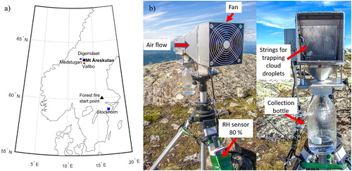
Rain and fog samples were collected at Åre (63̊ 26’ N, 13̊ 6’ E), Central Sweden (Figure 1a), during 27 June 2014 and 12 September 2014 (rain), and 4 July 2014 and 12 September 2014 (fog). Sixteen fog samples were collected at Mt Åreskutan station (1250 m above sea level a.s.l.), while 16 rain samples were collected at the foot of Mt Åreskutan (400 m a.s.l.) outside the village of Åre. In terms of air masses arriving to the site, the north-west sector represents clean Atlantic air, the south-east sector is characterized by air from densely populated and industrialized areas, and air masses coming from the north-east sector pass over boreal forests (Ogren and Rodhe, 1986; Drewnick et al., 2007; Franke et al., 2017). The mountainous area itself and its surroundings are considered rural areas; therefore no large local anthropogenic N_r sources are expected. The station is often within the planetary boundary layer (PBL) and surrounded by clouds, making it suitable for studying the partitioning of pollutants between rain and fog.

Fig. 1. (a) Map of central Sweden showing the sampling site, Mt Åreskutan (black square), the start point of the Västmanland forest fire (black triangle), Digernäset station (pale blue dot), Medstugan station (blue dot), Vallbo station (red dot) and Stockholm (blue square) for reference. (b) Custom-built active strand cloudwater collector (Collett et al., 1990) used during the CAEsAR 2014 campaign.

2.2. Sample collection and chemical analyses

Table 1 shows details on sample collection and analyses. The samples were collected at various intervals spanning from sub-daily collection to a continuous collection during 17 days, with an average collection interval of 5 days (Table 1). Before collection, sampling instruments and bottles were rinsed with ultrapure water (>18 MΩ·cm, Millipore Co.). Collection of samples was done in either high density polyethylene (HDPE, Nalgene) bottles or laboratory grade glass bottles (Duran^®), both materials present an inert behavior, e.g., ion exchange between the bottle material and the sample can be neglected.

Table 1. Sample type, ID, sampling period, and amount of water collected of rain and fog samples taken during the CAEsAR 2014 campaign.

Sample	ID	Sampling period in 2014	Sampling interval (days)	Total amount of water collected (ml)	Mean fog droplet Reff±1σ (μm)
Rain	R0	Jun 27–Jul 4	7	590	–
	R1	Jul 4–8	4	525	–
	R2	Jul 8–15	7	454	–
	R3*	Jul 15–17	2	3133*	–
	R4*	Jul 17–18	1	2518*	–
	R5▼	Jul 22–27	5	720	–
	R6▼	Jul 27	<1	173	–
	R7▼	Jul 27	<1	n.a.	–
	R8*▼	Jul 27–Aug 10	14	213*	–
	R9▼	Aug 10–14	4	56
	R10▼	Aug 14	<1	71	–
	R11▼	Aug 14–22	8	601*	–
	R12▼	Aug 22–23	1	2700	–
	R13▼	Aug 23–24	1	2980	–
	R14▼	Aug 24–Sep 10	17	715	–
	R15	Sep 10–12	2	118	–
Fog	F1	Jul 4–8	4	102	5.3 ± 2.2
	F2	Jul 8–14	6	378	8.6 ± 3.5
	F3	Jul 14–15	1	308	6.4 ± 2.7
	F4	Jul 15–17	2	287	8.9 ± 3.5
	F5	Jul 17–18	1	268	8.3 ± 4.2
	F6	Jul 18–19	1	96	7.1 ± 2.6
	F7▼	Jul 19–27	8	73	(**)
	F8▼	Jul 27–30	3	246	6.6 ± 2.7
	F9▼	Jul 30–Aug 10	11	472*	6.8 ± 3.1
	F10▼	Aug 10–12	2	217	5.9 ± 1.8
	F11	Aug 12–14	2	7	(**)
	F12▼	Aug 14–22	8	444*	9.0 ± 2.6
	F13▼	Aug 22–23	1	442	8.9 ± 2.2
	F14▼	Aug 23–24	1	241	9.5 ± 2.0
	F15▼	Aug 24–Sep 10	17	479*	8.2 ± 2.5
	F16▼	Sep 10–12	2	49	9.1 ± 2.2

(^▼) Samples in which nitrogen stable isotopes are measured; (*) volume corresponds to a fraction of total volume, i.e., the 5 L collection bottle was over-filled and part of the water was discarded; (n.a.) not available; and (**) R_eff below the cut-off size of the instrument. Samples in italics indicate that they were collected during the timespan of the forest fire in central Sweden.

Rain samples were collected in a 5 L plastic bottle using a wet-only sampler (M.I.C., Canada). Fog samples were collected in a pre-cleaned glass bottle with a custom-built single stage Caltech Active Strand Cloudwater Collector (Collett Jr. et al, 1990; Demoz et al., 1996) (Figure 1b), made with a stainless steel housing connected to fan rotating at 2000 min⁻¹. Air was pumped with a 5 m³ min⁻¹ flow through Teflon strings placed inside the housing to trap the fog drops by inertial impaction. The theoretical lower size cut-off of the instrument is 3.5 μm, based on droplet diameter (Collett et al., 1990). A switch turned on the fan only when relative humidity (RH) was above 80 %. After collection, rain and fog samples were filtered using Munktell quartz microfiber filters (T293, 47 mm diameter), poured in pre-cleaned plastic bottles and kept frozen (−20 °C) until chemical analyses. Blanks for the collection of fog (N = 2), rain (N = 3), and for the filtration processes (N = 1) were also obtained following the same procedure as for the samples (but with the fan turned off), using ultrapure water.

The samples were transported frozen (−20 °C) to the Department of Earth Sciences, Uppsala University, in order to analyze major ion concentrations (Na⁺, NH₄⁺, K⁺, Ca²⁺, Mg²⁺, Cl⁻, Br⁻, NO₃⁻, and SO₄²⁻) using a ProfIC850 Metrohm ion chromatograph (IC). Samples and standards were handled under a class 100 clean air hood, using powder-free gloves. Standards were prepared before analysis and stored frozen at −20 °C. Shortly prior to analysis, samples and standards were melted at room temperature (with vial lids closed), and then filtered using 0.2 μm polyethersulfone (PES) filters. Samples were placed in the IC auto-sampler, covered with aluminium foil to avoid any dust contamination. A minimum of 5 mL H₂O per sample was required to measure cations and anions. Calibration curves (R ≥ 0.9998) were constructed using 12 standards in the concentration range 1–1000 µg L⁻¹. Samples with ionic concentrations greater than the highest standard were diluted automatically using the Dosino module, which is part of the ProfIC850 chromatographic system. Three sample blanks consisting of ultrapure water were analysed at the beginning and the end of every sample batch. Check samples consisting of melted bulk snow collected in Uppsala, Sweden, were analysed every 10 samples to assess the reproducibility of measurements within a given batch. The reproducibility was within 5 % for each ion. Limits of Blank (LoB) (Armbruster and Pry (2008)) were calculated as the mean concentration plus 1.645 times one standard deviation (1σ) of six separate blanks, i.e., LoB = mean_blank + 1.645σ_blank, and were below 1 μmol L⁻¹ for each ion, while the Limits of Detection (LoD) (Armbruster and Pry (2008)) were calculated as LoB plus 1.645 times 1σ of six separate low concentration samples, i.e., LoD = LoB + 1.645σ_{low concentration sample}, and were below 1 μmol L⁻¹ for each ion.

Non-sea-salt (nss-), and sea-salt (ss-) fractions were calculated using the mean seawater composition with Na⁺ in seawater as reference ion, as follows: (1) $$\left[\text{ssX}\right] = k{\left[{\text{Na}}^{+}\right]}_{\text{total}}$$(1) (2) $$\left[\text{nssX}\right]={\left[\mathrm{X}\right]}_{\text{total}}-\left[\text{ssX}\right]={\left[\mathrm{X}\right]}_{\text{total}}-k{\left[{\text{Na}}^{+}\right]}_{\text{total}}$$(2) where X is an ion different from Na⁺, and (3) $$k=\frac{{\left[\mathrm{X}\right]}_{\text{seawater}}}{{\left[{\mathrm{N}\mathrm{a}}^{+}\right]}_{\text{seawater}}}$$(3) calculated using the standard mean chemical composition of seawater with a practical salinity of 35. Due to the relatively low concentrations of NH₄⁺ and NO₃⁻ in surface seawater (Summerhayes and Thorpe, 1996), NH₄⁺ and NO₃⁻ were not separated into nss- and ss-fractions (i.e., these ions were assumed to have a nss-origin only).

δ(¹⁵N), δ(¹⁷O) and δ(¹⁸O) of nitrate were analysed at the Stable Isotope Laboratory, University of East Anglia, using the denitrifier–thermal decomposition method (Casciotti et al., 2002; Kaiser et al., 2007). This method uses denitrifying bacteria (Pseudomonas aureofaciens) to convert NO₃⁻ into nitrous oxide (N₂O), followed by thermal decomposition in a gold tube at 880 °C, which is then introduced into a mass spectrometer to determine δ(¹⁵N), δ(¹⁷O) and δ(¹⁸O). The method requires a minimum of 10 nmol of NO₃⁻ (20 nmol being optimum) in at most 13 mL of sample. Consequently, samples R11–R14, which presented low NO₃⁻ concentrations, were pre-concentrated using lyophilisation following the procedure described by Vega et al. (2015). Considering that the observed range of δ(¹⁵N) in the samples is about 20 ‰, and that the concentration factors of the lyophilized samples were <10, any changes in δ(¹⁵N) due to sample pre-concentration are negligible compared to the environmental variability and can be disregarded. All samples were then filtered using 0.2 μm PES filters, collected in clean plastic tubes and kept frozen (−20 °C) until isotopic analysis. The ¹⁷O excess, Δ(¹⁷O), was calculated as Δ(¹⁷O) = δ(¹⁷O) − 0.52 δ(¹⁸O). δ(¹⁵N) and δ(¹⁸O) values were corrected for the contribution of ¹⁴N¹⁴N¹⁷O to the peak at mass 45 using δ(¹⁷O). Standard deviations were 0.3 ‰, 0.4 ‰, and 0.5 ‰ for δ(¹⁵N), δ(¹⁸O), and Δ(¹⁷O), respectively. Samples R12–R14 had low volume left for isotope analysis, thus, only δ(¹⁵N) and δ(¹⁸O) could be analysed. Τhe ¹⁷O peak area of samples R11, F12 and F13 was too low, thus the mean Δ(¹⁷O) value of the series was assigned to these samples.

2.3. Rain deposition

Since rain samples were collected at different sampling intervals, mean daily precipitation (P_d) was estimated using daily precipitation data provided by the Swedish Meteorological and Hydrological Institute (SMHI, http://opendata-download-metobs.smhi.se) for three meteorological stations (Medstugan, Digernäset, and Vallbo) located nearby the study site (Figure 1a). Of the 77-day campaign period, only 58 days had precipitation (Table S1, in the supplementary material). The daily ionic rain deposition (D_rain, in µmol m⁻² d⁻¹) was then calculated as follows: (4) $$D_{\text{rain}}={ c}_{\mathrm{i}}\times P_{\mathrm{d}}$$(4) where c_i is the ionic concentration, in µmol L⁻¹, measured in rain samples, and P_d the mean daily precipitation, in mm d⁻¹ (Table S1). Even though we can approximately know the amount of daily precipitation by using the station data, since each rain sample corresponds to various days in which precipitation was collected, it is not possible to know if the ion concentrations vary from one collection day to another. Consequently, the calculation of D_rain was done assuming that the ionic concentration during different days, within the same collection interval and rain sample, remained constant.

2.4. Fog deposition

Ion deposition by fog (D_fog, in µmol m⁻² d⁻¹) was estimated as: (5) $$D_{\text{fog}}=86400\times \frac{\gamma \left({\mathrm{H}}_2\mathrm{O}\right)}{\rho \left({\mathrm{H}}_2\mathrm{O}\right)}\times v\times c_{\mathrm{i}}$$(5) where 86400 is a conversion factor for units (e.g., number of seconds in one day (s d⁻¹)), γ(H₂O) is the mean liquid water mass concentration in air (or liquid water content; LWC) (in g m⁻³) corresponding to each fog event (Table S2), ρ(H₂O) is the density of liquid water (in kg L⁻¹), v is the mean deposition velocity of fog droplets (in m s⁻¹) during each fog event, and c_i is the ionic concentration (in µmol L⁻¹) measured in each fog sample. LWC was obtained using laser-diffraction measurements at 5-min averages, and readings were only considered during periods in which the sampling location was within the cloud. D_fog depends on droplet size through the v parameter. The effective radius (R_eff) of fog droplets corresponding to each fog event was obtained using a particulate volume monitor (PVM; Gerber, 1991) at a 1-min time resolution. Mean R_eff values are shown in Table 1. Two fog samples (F7 and F11) had mean R_eff below the fog collector cut-off size, therefore, we did not considered those samples in the D_fog calculations. We used modelled cloud droplet deposition velocities reported by Matsumoto et al. (2011) for particles with radii larger than 1.75 μm (cut-off of the fog collector) and smaller than 15 μm (i.e., v = 0.047  m  s⁻¹ for 1.75 μm<R_eff<2.5 μm; v = 0.101  m  s⁻¹ for 2.5 μm<R_eff<5 μm; v = 0.135 m s⁻¹ for 5 μm<R_eff<10 μm; and v = 0.156 m s⁻¹ for 10 μm<R_eff<15 μm). We then assigned deposition velocities to each R_eff value measured at 1-min resolution. The LWC and v values were then averaged and used in equation (5)(5) $$D_{\text{fog}}=86400\times \frac{\gamma \left({\mathrm{H}}_2\mathrm{O}\right)}{\rho \left({\mathrm{H}}_2\mathrm{O}\right)}\times v\times c_{\mathrm{i}}$$(5) . The D_fog values reported in this study contain uncertainties related to the variables in equation (5)(5) $$D_{\text{fog}}=86400\times \frac{\gamma \left({\mathrm{H}}_2\mathrm{O}\right)}{\rho \left({\mathrm{H}}_2\mathrm{O}\right)}\times v\times c_{\mathrm{i}}$$(5) , especially the selection of v values, in addition to the intrinsic fog collection efficiency of the instrument used in this study.

Table 2. Mean molar concentrations, standard deviation (1σ), 25^th, 50^th, and 75^th percentiles of selected ions, δ(¹⁵N), δ(¹⁸O), δ(¹⁷O), and Δ(¹⁷O) in rain and fog samples.

	N	Mean ± 1σ	25^th	50^th	75^th	N	Mean ± 1σ	25^th	50^th	75^th	Ratio fog/rain ± 1σ
		Rain (μmol L^−^1)					Fog (μmol L^−^1)
Na^+	16	7 ± 8	2	3	9	16	53 ± 139	4	10	23	8 ± 22
Cl^−		7 ± 9	2	3	12		32 ± 55	4	9	31	5 ± 9
Mg^2+		2 ± 2	0	1	3		8 ± 14	2	4	8	4 ± 8
NH4^+		9 ± 8	5	8	12		25 ± 32	9	17	28	3 ± 4
Br^−		0.03 ± 0.02	0.01	0.02	0.04		0.08 ± 0.09	0.01	0.05	0.10	3 ± 3
NO3^−		11 ± 10	4	8	17		35 ± 56	13	20	36	3 ± 6
SO4^2−		9 ± 10	3	6	9		24 ± 26	7	17	27	3 ± 4
K^+		2 ± 1	1	1	2		3 ± 5	1	2	3	2 ± 3
Ca^2+		17 ± 19	5	10	23		14 ± 27	3	5	11	1 ± 2
ssK^+		0.1 ± 0.2	0	0.1	0.2		1 ± 3	0.1	0.2	0.5	10 ± 36
ssCa^2+		0.1 ± 0.2	0	0.1	0.2		1 ± 3	0.1	0.2	0.5	10 ± 36
ssMg^2+		0.8 ± 0.9	0.2	0.3	1.0		6 ± 15	0	1	3	8 ± 21
ssSO4^2−		0.4 ± 0.5	0.1	0.2	0.6		3 ± 8	0	1	1	8 ± 22
nssMg^2+		1 ± 8	0	1	2		3 ± 2	2	2	4	3 ± 24
nssSO4^2−		8 ± 10	3	6	8		21 ± 21	6	13	27	3 ± 4
nssK^+		2 ± 1	1	1	2		2 ± 3	1	2	3	1 ± 2
nssCa^2+		17 ± 18	5	10	23		12 ± 25	3	5	11	1 ± 2
		Rain (‰)					Fog (‰)				Δδ (fog − rain)
δ(^15N)	9	−2 ± 8	−7	−7	5	9	−8 ± 2	−9	−8	−6	−6 ± 8
δ(^18O)	9	57 ± 15	42	66	67	9	71 ± 3	69	71	73	14 ± 15
δ(^17O)	6	59 ± 3	58	58	60	9	62 ± 5	61	64	65	3 ± 6
Δ(^17O)	6	22 ± 1	22	22	22	9	25 ± 2	25	25	25	3 ± 2

Fog/rain ratios of mean values are also shown. N indicates the number of samples collected and analysed. Percentiles for ssK⁺ and ssCa²⁺ in fog are shown with one decimal as an exception for visualization.

2.5. Air mass back-trajectory analyses

We used a reconstruction of air mass back-trajectories with the NOAA Hybrid Single-Particle Lagrangian Integrated Trajectory model (HYSPLIT) (Draxler and Hess, 1998; Draxler, 2004) in order to understand the medium- and long-range transport of aerosols and the influence of different source regions of air masses arriving to the sampling site. The calculations were based on meteorological data from NCEP’s (National Weather Service’s National Centres for environmental Prediction) Global Data Assimilation System (GDAS) with 1-degree resolution. Air masses were modelled at an elevation of 500 m above ground level with 7-day back-trajectory runs with a restart interval of 48 h. The length of the back-trajectories was chosen based on the estimated lifetime of NO_x in Arctic regions, i.e., ∼10 days (Liu et al., 1987), and the global mean lifetime of NO₃⁻ aerosol, i.e., 4–6 days (Xu and Penner, 2012).

3. Results and discussion

3.1. Ion concentrations and nitrate stable isotope values

Table 2 shows mean molar concentrations of major ions (ss- and nss-fractions), standard deviation (1σ), and the 25^th, 50^th and, 75^th percentiles for rain and fog samples. The 50^th percentile corresponds to the median and the 25^th and 75^th percentiles, i.e., lower and upper percentiles are located half-way between the median and the data extremes presented in Table 2, represent a robust and resistant measure of central tendency and spread of the data (Wilks, 2006). For the sake of comparativeness, we conducted our analysis using mean concentration values. It is worth saying that some of the references used in this study only report mean concentration or deposition values and the 25^th, 50^th, and 75^th percentiles (e.g., Jung et al., 2013), mean, standard deviation, and the 25^th, 50^th, and 75^th percentiles (Franke et al., 2017), median and extreme values (e.g., Ogren and Rodhe, 1986), mean and extreme values (Zimmermann and Zimmermann, 2002; Lange et al., 2003), or did not report any statistics, either robust or nonrobust, to account for spreading of the data (e.g., Ogren and Charlson, 1984; Ferm et al., 2000). Our data sets are physically constrained to lie above a minimum value (i.e., precipitation, ion concentrations and deposition fluxes, cannot take negative values), therefore, the datasets would be more likely positively skewed. To test the symmetry of our data sets, we employed the Yule-Kendall index, which is a robust and resistant alternative to the skewness coefficient (Wilks, 2006). The results of the test show that major ion (Na⁺, Cl⁻, Mg²⁺, NH₄⁺, Br⁻, NO₃⁻, SO₄²⁻, K⁺, and Ca²⁺) concentration data for rain and fog have Yule-Kendall index values above zero, which indicates that the data sets are right-skewed as expected. In rain, molar mean values were in the range of 0.1–17 μmol L⁻¹, with the exception of Br⁻ that showed average concentrations two orders of magnitude lower than the other ions. Meanwhile, in fog, mean values were in the range of 1–53 μmol L⁻¹, with Br⁻ also exhibiting mean concentrations two order of magnitude lower than the other ions. The fog/rain ratio in Table 2 shows that mean concentrations of most ions were 2–8 times higher in fog than in rain, with the exception of nssK⁺, and nssCa²⁺ which showed similar values in both rain and fog.

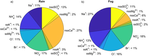
NO₃⁻ made up a larger proportion of total inorganic nitrogen ions (NO₃⁻ + NH₄⁺, NO₂⁻ was not analyzed) than NH₄⁺ in both rain and fog samples. Figure 2 shows the contribution of each ion to the total load of ions in rain and fog samples. For both rain and fog samples, total inorganic nitrogen contributes about (31 ± 25) % and (31 ± 42) % of the total ion load, respectively. nssCa²⁺ was the dominant ion in rain samples (27 ± 31) %, with NO₃⁻, NH₄⁺, nssSO₄²⁻, Na⁺, and Cl⁻ also having individual contributions above 10 %. In fog, Na⁺ was the dominant ion (27 ± 75) %, followed by NO₃⁻, Cl⁻, NH₄⁺, and nssSO₄²⁻ with individual contributions above 10 %.

Fig. 2. Pie-plot of ion fractions (mol-%) measured in (a) rain and (b) fog samples during the CAEsAR campaign. Nss- and ss-fractions were calculated as explained in Section 2.2.

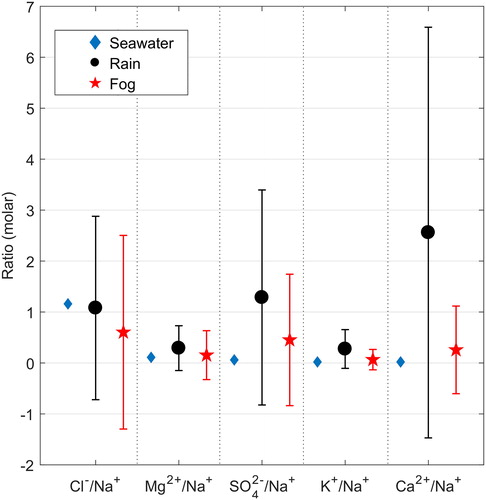
Figure 3 shows the sea-salt molar ratios referred to Na⁺ in bulk seawater, rain, and fog (ratios were calculated using mean ion concentrations). The Cl⁻/Na⁺ ratio in rain and fog is lower than in seawater. For the other ions, ratios in rain and fog are higher than in seawater indicating a dominance of non-sea salt sources, which can be also observed in the mean ion concentrations presented in Table 2.

Fig. 3. Sea-salt ratios referred to Na⁺ in bulk seawater (blue diamonds), in rain (black circles) samples, and in fog (red stars) samples collected during the CAEsAR campaign. Fog/rain ratios were calculated using mean ion concentrations. Error bars represent 1σ.

For stable isotopes of nitrogen and oxygen in nitrate, there is a difference of (6 ± 8) ‰ between mean δ(¹⁵N) values in fog (i.e., (−8 ± 2) ‰) compared to values in rain samples (i.e., (−2 ± 8) ‰), while there is a difference of (14 ± 15) ‰ between mean δ(¹⁸O) values in fog (i.e., (71 ± 3) ‰) and rain (i.e., (57 ± 15) ‰) (Table 2). Both δ(¹⁵N) and δ(¹⁸O) presented values within ranges previously reported for atmospheric NO₃⁻ (Heaton et al., 1987; Hastings, 2010 and references therein; Vega et al., 2015).

3.2. Sources

In order to assess possible sources explaining the total variance in the ion concentrations from both rain and fog samples, a principal component analysis (PCA) was applied to the different ion series. For the PCA analysis, ion concentrations were log-normalised by taking their logarithms, subtracting the mean of the data series from each data point and then dividing the result by the standard deviation of the data series. PCA analyses were performed using ion concentration of samples listed in Table 1, at a resolution corresponding to each sampling interval. The sum of the variances of the first three principal components (PC1, PC2, and PC3) was ≥ 80  % of the total variance of the original rain and fog series. Principal components are shown in Table 3. PCA results are consistent between rain and fog samples, and show that all selected ions contribute similarly to most of the variance in the samples (PC1). The loadings in PC2 for rain, show that an independent source of NO₃⁻ and NH₄⁺ (e.g., the effect of the large forest fire occurred in central Sweden during the sampling period, industrial NO_x emissions and/or soil emissions form fertilized areas) could explain on the order of 12 % of the total variance, while the loadings in PC3 show that an independent source of Br⁻ (not linked with sea-salts) could explain near 5 % of the total variance, e.g., from methyl bromide used for agricultural fumigation purposes. In the case of the fog samples, PC1 is similar as for rain samples, while PC2 suggest a source of NH₄⁺. PC3 shows a source of nssMg²⁺ dominating this component, likely the input of mineral dust from the mountaintop.

Table 3. PCA loadings of the first three principal components calculated using concentrations of major ions (separated into ss- and nss-fractions) measured in rain and fog samples collected during the CAEsAR 2014 campaign.

Sample	Rain			Fog
Loadings	PC1	PC2	PC3	PC1	PC2	PC3
Na^+	0.30	−0.23	−0.02	0.32	−0.19	−0.02
NH4^+	0.23	0.45	−0.36	0.22	0.45	−0.33
ssK^+	0.30	−0.23	−0.02	0.32	−0.19	−0.02
ssCa^2+	0.30	−0.23	−0.02	0.32	−0.19	−0.02
ssMg^2+	0.30	−0.23	−0.02	0.32	−0.19	−0.02
Cl^−	0.30	−0.13	0.12	0.30	−0.28	0.06
Br^−	0.20	0.25	0.90	0.12	−0.38	−0.31
NO3^−	0.26	0.42	0.01	0.31	0.20	2 × 10^−3
ssSO4^2−	0.30	−0.23	−0.02	0.32	−0.19	−0.02
nssK^+	0.29	−0.15	−0.10	0.26	0.33	0.02
nssCa^2+	0.30	−0.02	−0.04	0.28	0.31	0.25
nssMg^2+	0.25	0.32	−0.12	0.19	0.13	0.74
nssSO4^2−	0.27	0.37	−0.13	0.21	0.37	−0.42
Explained Variance (%)	79	12	5	67	16	7
Source	Mixed	Soil/Industrial Forest fire	Fumigation	Mixed	Soil/Industrial	Mineral dust

Possible sources related to the different components are displayed in the bottom row.

Figure 4 shows NH₄⁺, NO₃⁻, and Na⁺ concentrations, and Figure 5 shows Br⁻, nssMg²⁺, nssSO₄²⁻, and K⁺ concentrations, in individual rain and fog samples collected during the CAEsAR campaign. Note that the concentrations were plotted in such a way that each collection interval for rain overlaps the correspondent collection period for fog (e.g., R1 was collected in the same period as F1, R5 in the same period as F7, and no fog samples were collected during the collection period of sample R0). In case of samples R6 and R7, both overlap with sample F8 (the overlapping is indicated with horizontal arrows in Figures 4 and 5); while samples R9 and R10 together overlap with F10 and F11. We divided the samples into periods in which NH₄⁺ and NO₃⁻ concentrations were more than double the mean (high), within twice the mean and half the mean (medium), or less than half the mean (low) (Table 4). In general, most of rain samples presented NH₄⁺ concentrations classified as medium (samples R0, R2–R10, and R15). One sample had NH₄⁺ concentration classified as high (sample R1), while four samples had concentrations classified as low (samples R11–R14). There was a general correspondence between NH₄⁺ and NO₃⁻ concentration categories in rain (Table 4), although NO₃⁻ had two additional samples with concentrations classified as high (samples R9 and R15); and two additional samples classified as low (samples R3 and R4). Conversely, only eight fog samples presented NH₄⁺ concentrations classified as medium (samples F2–F4, F6, F8–F10, and F16), while only one sample presented NH₄⁺ and NO₃⁻ concentrations classified as high (sample F1) (Table 4).

Fig. 4. Stacked bar plot of NH₄⁺, NO₃⁻, and Na⁺ concentrations in each (a) rain and (b) fog sample collected during the CAEsAR campaign. Horizontal arrows indicate that samples R6 and R7 overlap with sample F8; while samples R9 and R10 together overlap with sample F10 and F11. For sample collection periods see Table 1.

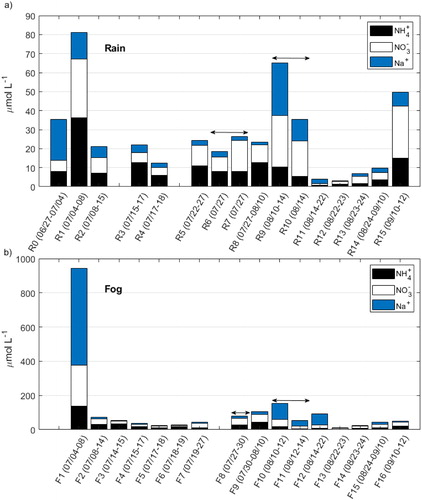
Fig. 5. Stacked bar plot of Br⁻, nssMg²⁺, nssSO₄²⁻, and K⁺ concentrations in each (a) rain and (b) fog sample collected during the CAEsAR campaign. Note that Br⁻ concentrations have been scaled to improve visualization. Horizontal arrows indicate that samples R6 and R7 overlap with sample F8; while samples R9 and R10 together overlap with sample F10 and F11. For sample collection periods please refer to Table 1.

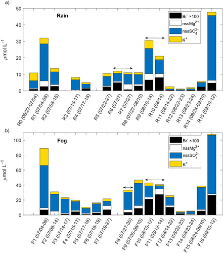
Table 4. Rain and fog sample classification considering concentrations thresholds; more than double the mean (high), less than half the mean (low), and within twice the mean and half the mean (medium).

Sample Rain (Fog)	Rain		Fog
	NH4^+	NO3^−	NH4^+	NO3^−
R0	medium		(*)
R1 (F1)	high
R2 (F2)	medium
(F3)	(*)		medium	low
R3 (F4)	medium	low	medium	low
R4 (F5)	medium	low
(F6)	(*)		medium	low
R5 (F7)	medium		low	medium
R6	medium		(*)
R7 (F8)	medium
R8 (F9)	medium
R9 (F10)	medium	high	medium
R10 (F11)	medium		low
R11 (F12)	low			medium
R12 (F13)	low
R13 (F14)	low
R14 (F15)	low			medium
R15 (F16)	medium	high	medium

Rain and fog samples collected within the same time interval are shown together. (*) no sample.

Air mass back-trajectories showed that rain samples with NO₃⁻ concentrations classified as high, and NH₄⁺ concentrations ranging from medium to high (Table 4), had a common origin over industrialized regions or over the North Atlantic Ocean (Figure 6a, b, and d, i.e., samples R1, R9, and R15). In the case of sample R1, ssK⁺, ssCa²⁺, nssCa²⁺, nssMg²⁺ and nssSO₄²⁻ concentrations were also categorised as high; for R9, all ions but nssK⁺ and nssSO₄²⁻ had concentrations classified as high. For R15, only nssSO₄²⁻ concentrations were considered high. Therefore, we consider ion concentrations in samples classified as high to have mainly an anthropogenic influence. This is in agreement with pollution episodes evidenced by Franke et al. (2017) during July 3–12 corresponding to samples R1 and F1 (Figure 5a), which also show large rain daily deposition fluxes of nssSO₄²⁻ (Figure 7b), and the pollution event registered during September 7–10 corresponding to sample F15 explained further.

Fig. 6. 7-day back-trajectories arriving to Åreskutan for samples (a) R1, (b) R9, (c) R8, (d) R15, (e) R12, and (f) R13. Start altitude is an elevation of 500 m above ground level (a.g.l.). Each colour represents a back-trajectory restarted each 48 h: initial back-trajectory (red line and triangles), restarted after 48 h (blue line and squares), and restarted after 96 h (green line and circles).

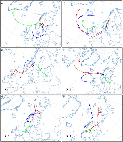
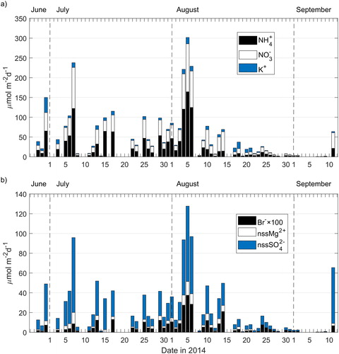
Fig. 7. Stacked bar plot of (a) NH₄⁺, and NO₃⁻, and (b) Br⁻, nssMg²⁺, and nssSO₄²⁻ daily rain deposition obtained as explained in Section 2.3. Note that Br⁻ concentrations have been scaled to improve visualization.

On the other hand, rain samples with NO₃⁻ concentrations classified as low, and NH₄⁺ concentrations ranging from low to medium (Table 4), originated from three sectors: the Atlantic Ocean, the Arctic, and the Baltic area (Figure S1). In addition to low inorganic nitrogen concentrations found in these samples, Br⁻, nssMg²⁺, and nnsSO₄²⁻ concentrations were also generally low or medium. Therefore, we consider samples with inorganic nitrogen concentrations classified as low to have marine (Figure S1: samples R3, R4, and R14) and Arctic (Figure S1: R11, Figure 6: R12, and R13) origins.

Back-trajectories for samples with NO₃⁻ and NH₄⁺ concentrations classified as medium (Table 4) showed inland air masses traveling within Scandinavia (Figure S2: samples R2, R6, and R7), with some of the trajectories reaching over the Atlantic Ocean (Figure S2: samples R0, R5, and Figure 6: sample R8). This air mass classification based on ion concentration thresholds agree with the results by Franke et al. (2017) for air masses arriving Mt Åreskutan during the CAEsAR campaign period.

3.2.1. Forest fire

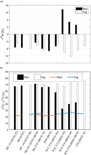
Franke et al. (2017) reported that the plume of a forest fire originated in Västmanland, Central Sweden (Figure 1a), which started on July 31 and was controlled by August 11 (MSB, 2015). The plume of the forest fire reached the mountain top during August 2–5, evidenced by high organic carbon (OC), elemental carbon (EC), and K⁺ concentrations measured in particulate matter sampled at the top of Mt Åreskutan. Daily rain deposition (Figure 7) showed high NH₄⁺ and NO₃⁻ deposition during August 4–6 (corresponding to sample R8), which could be associated to the forest fire plume. nssSO₄²⁻ and Br⁻ rain deposition fluxes were also high during this event. Conversely to the findings by Franke et al. (2017), rain deposition of K⁺ did not show maximum values during the mentioned period. Figure 8 shows δ(¹⁵N), δ(¹⁸O), and Δ(¹⁷O) measured in rain and fog between July 22 and September 12, 2014. NO_x emissions from forest and grassland fires generate NO₃⁻ aerosol bearing δ(¹⁵N) values in the range of −7.2 to 25.7 ‰ (Hastings, 2010; Fibiger and Hastings, 2016). NO₃⁻ measured in Svalbard ice cores has been linked to Siberian forest and grassland fires evidenced by a marked increase in δ(¹⁵N) values (i.e., less negative values corresponding to an enrichment in the ¹⁵N isotope) (Vega et al., 2015). Rain samples show a difference of ∼3 ‰ (less negative δ(¹⁵N) values) between sample R8 (i.e., −5 ‰) and samples for late-July (R6, i.e., −7 ‰) and mid-August (R9, i.e., −8 ‰) in Figure 8a, respectively. This difference could be due to the influence of NO₃⁻ enriched in the ¹⁵N isotope and emitted by the Västmanland forest fire. δ(¹⁵N) in fog shifted to less negative values with a difference of 2 ‰ and 3 ‰ between sample F9 (i.e., −6 ‰) and samples for late-July (F8, i.e., −8 ‰) and mid-August (F10, i.e., −9 ‰), however, not reaching a minimum value as was the case with sample R8 in the rain samples set, while δ(¹⁸O) and Δ(¹⁷O) in both, rain and fog, did not experienced any particular change that could be attributed to the forest fire plume influence during those days (samples R8 and F9 in Figure 8b).

Fig. 8. Bar plot of (a) δ(¹⁵N), and (b) δ(¹⁸O) and Δ(¹⁷O) in NO₃⁻, from rain and fog samples collected during the CAEsAR campaign. In the bottom graph, Δ(¹⁷O) values for rain and fog samples are shown with red and blue lines, respectively. (*) The sampling date is (as detailed in Table 1): R5 07/22–27, R7 07/27, F9 07/30–08/10, F10 08/10–12.

3.2.2. Kola Peninsula and oil rig emissions

A sharp increase of ∼21 ‰ in δ(¹⁵N) toward positive values was observed in rain samples, between sample R11 (i.e., −7 ‰) and R12 (i.e., 14 ‰), with positive δ(¹⁵N) maintained during the period August 22–September 10 (samples R12–R14 in Figure 8a). These samples had NO₃^– and NH₄⁺ concentrations classified as low (Table 4), and air mass back-trajectories for the period covered by the samples had a north to north-east origin (e.g., Figure 6e and f). These back-trajectories show that air masses travelled over Kola Peninsula, Russia, where several industrial NO_x sources exist (Prank et al., 2010; Hongisto, 2015). In addition, Franke et al. (2017) reported high EC to OC mass concentration ratios during August 20–23, associated with air masses arriving from the north, with PBL residence times above oil rigs off the Norwegian coast. These rigs emit NO_x (Lee et al., 2015) from combustion processes, and therefore, with expected δ(¹⁵N) values close to those reported for combustion of fossil fuels. To our knowledge, there are no studies of δ(¹⁵N) in the oil rig plume NO_x. Therefore, considering the isotopic fingerprint of reported mobile and stationary NO_x sources, the δ(¹⁵N) of oil rig emissions could be within a wide range between −13 and 20 ‰ (Hastings (2010) and references therein; Felix et al., 2012; Miller et al., 2017). Concomitant to the shift in δ(¹⁵N) values, a decrease in δ(¹⁸O) values from 58 ‰ to 33 ‰ in rain samples was observed between samples R11 and R12 (Figure 8b), which could be due to formation of NO₃⁻ via oxidation of NO_x with hydroxyl radicals (OH) in competition with NO_x oxidation by O₃, leading to δ(¹⁸O) values in NO₃⁻ below 50 ‰ (Burns and Kendall, 2002; Williard et al., 2001).

On the other hand, samples R1, and R9–R10 show medium to high NH₄ and NO₃, but no positive δ¹⁵N. In addition, sea-salt (Na⁺) concentrations measured in these samples have medium (R10) to high (R1 and R9) values (Figure 4a). Back-trajectories for these samples show air masses travelling from the south-west sector to the study site (Figure 6a and b, and Figure S2f). Figure 7 in Franke et al. (2017) shows major offshore oil rig installation over Northern Europe. We hypothesize that medium to high inorganic nitrate in these samples may originate from oil rigs located in the Northern Sea, which would explain also the enrichment in sea-salts observed in these samples.

3.2.3. Volcanic emissions

Grahn et al. (2015) reported the presence of sulfur gases detected on September 10 at Västerbotten county, approximately 250 km to the north east of Åre due to degassing of the Icelandic Bardarbunga volcano. nssSO₄²⁻ concentrations in rain and fog (samples R15 and F16, Figure 5a and b), and rain nssSO₄²⁻ deposition showed high values during September 11 (Figure 7b), which could be attributed to the passing of the volcanic plume over Åre. This is supported by the air mass back-trajectory for that period (Figure 6d) which shows transport pathways from Iceland to central Sweden.

3.3. Scavenging of ions

As noted in Section 3.1, mean concentrations of ions showed higher values in fog than in rain (Table 2), which suggest that scavenging of ions per unit of cloud water deposited by wet deposition was more efficiently done by fog than by rain (with the exception of Ca²⁺), as expected for water-soluble ions (Lange et al., 2003; Gilardoni et al., 2014). NH₄⁺ and NO₃⁻ showed similar (statistically significant at 95  % confidence interval when using a Wilcoxon rank-sum test (Gibbons and Chakraborti, 2003)) fog/rain ratios of mean concentrations (Table 2). The highest partition between fog and rain was registered for sea-salts Na⁺ (fog/rain ratio: 8 ± 22), ssK⁺ (10 ± 36), ssCa²⁺ (10 ± 36), ssMg²⁺ (8 ± 21), and ssSO₄²⁻ (8 ± 22), most likely associated with the presence of these ions in coarse form, as for example in sea-salt aerosols acting as fog condensation nuclei (Sasakawa et al., 2003), supporting the assumption that Na⁺ in the samples was mostly originated by sea-salts (Section 2.2). Jung et al. (2013) have found that there is a preferential behavior for coarse particles to act as condensation nuclei in sea fog, with NO₃⁻ being scavenged more efficiently than NH₄⁺.

Table 5 shows fog/rain ratios of mean ion concentrations of samples classified as high, medium, or low (explained in Section 3.2.), and associated to three main ion sources: anthropogenic (i.e., high NO₃⁻ concentrations), inland (i.e., medium NO₃⁻ concentrations), and marine Arctic (i.e., low NO₃⁻ concentrations) (also described in Section 3.2.). Sea-salt ions present similar ratios within each group, with ratios associated to anthropogenic sources being larger than ratios of marine Arctic sources, and larger than inland sources (with the exception of Cl⁻ that shows lower values than the other sea-salt ions in samples associated with anthropogenic and inland sources). The lower Cl⁻ ratio could be due to the volatilization of sea-salt Cl⁻ as HCl, which would be enhanced by the presence of HNO₃ and H₂SO₄; consequently, it could be expected that Cl⁻ loss would be enhanced by the presence of anthropogenic aerosol. There is a clear difference between the ratios for sea-salt fractions and non-sea-salt fractions (Table 5). In samples associated to anthropogenic sources, ratios for the same ion are higher in the sea-salt fraction than in the non-sea-salt fraction. This could indicate that fog scavenges non-sea-salt fractions less efficiently than sea-salt fractions in air masses with anthropogenic origin. Non-sea-salt fractions of K⁺, Ca²⁺, and Mg²⁺ are often associated with crustal emissions. Or, alternatively, that crustal aerosols were below the altitude at which the fog developed at Mt Åreskutan, hence, those would not be scavenged by fog, and concentrations would be depleted in fog samples compared to rain, with rain washing out particles below cloud level.

Table 5. Fog/rain ratios of mean ion concentrations of samples classified as high, medium, or low (explained in Section 3.2), and associated to three main ion sources: anthropogenic (i.e. high NO₃⁻ concentrations), inland (i.e. medium NO₃⁻ concentrations), and marine Arctic (i.e low NO₃⁻ concentrations), also described in Section 3.2.

Ion	Ratio fog/rain ± 1σ
	Anthropogenic	Inland	Marine Arctic
Na^+	14 ± 20	2 ± 3	7 ± 12
NH4^+	3 ± 4	3 ± 2	2 ± 3
ssK^+	14 ± 20	2 ± 3	7 ± 12
ssCa^2+	14 ± 20	2 ± 3	7 ± 12
ssMg^2+	12 ± 18	2 ± 3	7 ± 12
Cl^−	5 ± 6	3 ± 3	7 ± 14
Br^−	4 ± 3	3 ± 4	6 ± 10
NO3^−	4 ± 4	3 ± 2	4 ± 3
ssSO4^2−	14 ± 20	2 ± 3	7 ± 12
nssK^+	2 ± 2	1 ± 1	1.4 ± 0.8
nssCa^2+	1 ± 1	0.8 ± 0.7	0.6 ± 0.6
nssMg^2+	0.8 ± 0.4	4 ± 3	8 ± 8
nssSO4^2−	2 ± 2	3 ± 2	5 ± 6

In the case of nssMg²⁺, the ratio found in air masses associated with marine-Arctic origins, was almost twice the ratio for the sea-salt fraction. This could be attributed to sources of nssMg²⁺ with no crustal origin, due to the fact that other crustal ions do not show high fog/rain ratios (e.g., nssK⁺ nor nssCa²⁺). Kindbom et al. (1993) reported point sources of Mg²⁺ (i.e., steel industry, forest industry, and cement industry) and areal sources (i.e., wood/bio-fuel, oil, and coal) in Sweden. Marine Arctic air masses passed over large mining and industrial areas located in Northern Sweden; therefore, it is plausible that nssMg²⁺ aerosol generated by those activities could had been transported to Mt Åreskutan and scavenged preferably by fog than rain.

Ratios for Br⁻ are also high for marine Arctic air masses, which could be due to non-sea-salt sources. There are multiple sources of bromine that could eventually generate Br⁻ in the troposphere. Wetlands are a natural source and sink of methyl bromide (CH₃Br) to the atmosphere, with net uptake found for wetlands located in Northern Sweden (Hardacre et al., 2009). In addition, anthropogenic organic and inorganic brominated compounds are mainly used in agriculture and paper-cellulose industry, respectively, as fungicide and algaecide (KEMI-report, 2014). However, it is not possible to assess with the current data if Br⁻ measured in rain and fog is mainly from natural, agricultural, or industrial sources; this question remains for future work on the area, considering the presence of wetland, forest plantations, and at least four cellulose factories north-east of the sampling site (SkogsIndustrierna, 2018).

3.4. Rain deposition

Mean precipitation during the sampling period was (2 ± 3) mm (with 58 registered precipitation events within the 77-day sampling period, Table S1). A precipitation event was considered as “large” when the precipitation amount was above the mean precipitation value plus twice the standard deviation (i.e., 8 mm). Therefore, according to the station data, large precipitation events were observed in the region during July 17, August 4–6, and August 18. Table 6 shows mean and 1σ of rain deposition, in μmol m⁻² d⁻¹, of major ions sampled at Mt Åreskutan. Mean rain deposition of NH₄⁺ and NO₃⁻ was (26 ± 36) μmol m⁻² d⁻¹ and (23 ± 27) μmol m⁻² d⁻¹, respectively, representing (36 ± 37) % of the total major ion rain deposition flux. Ca²⁺ contributed with the largest individual percentage to the total flux (25 ± 30) %, while Na⁺ and Cl⁻ contributed together with (22 ± 26) % of the total rain deposition flux, and SO₄²⁻ contributed with (12 ± 15) %, with the remaining ions, K⁺, Mg²⁺, and Br⁻, contributing less than 10 % altogether.

Table 6. Mean and standard deviation (1σ) for rain and fog deposition of selected ions considering modelled deposition velocities reported by Matsumoto et al. (2011).

Ion	Rain deposition (μmol m^−2 d^−1)	Fog deposition (μmol m^−2 d^−1)
Na^+	15 ± 26	113 ± 268
NH4^+	26 ± 36	72 ± 69
K^+	5 ± 6	9 ± 10
Ca^2+	34 ± 38	33 ± 57
Mg^2+	4 ± 5	18 ± 27
Cl^−	15 ± 19	70 ± 114
Br^−	0.06 ± 0.08	0.2 ± 0.3
NO3^−	23 ± 27	89 ± 111
SO4^2−	17 ± 19	75 ± 92

Daily rain deposition of NH₄⁺, NO₃⁻, Br⁻, nssMg²⁺, and nssSO₄²⁻ are shown in Figure 7. Rain deposition was highly variable during the campaign depending on ion concentration and precipitation amount. Of the three large precipitation events registered in the station data (i.e., more than 10 mm per day, Table S1), only two of them showed increased NH₄⁺ and NO₃⁻ fluxes (i.e., on July 17, and August 4–6, Figure 7). The largest rain deposition events (i.e., on July 7, and August 4–6, Figure 7) correspond to anthropogenic and inland air mass back-trajectories. Those two events represented 8 % and 27 % of the total load of NH₄⁺ and NO₃⁻ during the whole campaign period.

3.5. Fog deposition

Deposition of major ions by fog was estimated using the approximation described in Section 2.4. Table 6 shows mean and 1σ of fog deposition, in μmol m⁻² d⁻¹, of major ions sampled at Mt Åreskutan. Due to the crude assumptions made in estimating fog deposition (Section 2.4), fog deposition rates are highly uncertain. Considering the D_fog values shown in Table 6, Na⁺ showed the highest individual contribution, contributing a (24 ± 60) % on a mole per mole basis. NH₄⁺ and NO₃⁻ accounted for (34 ± 36) %, Na⁺ and Cl⁻ together contributed (38 ± 66) %, SO₄²⁻ contributed (16 ± 22) %, with the remaining ions contributing less than 12 % altogether. NH₄⁺ and NO₃⁻ deposited by fog would represent (77 ± 80) % of total inorganic nitrogen wet deposition (i.e., rain deposition + fog deposition), which greatly surpasses the fraction of total inorganic nitrogen deposited by wet deposition. Wet deposition and total deposition of NH₄⁺ and NO₃⁻ have been estimated over Sweden during 1997 and presented in a report by the Swedish Environmental Protection Agency (Bertills and Näshol, 2000, Report 5067). Wet and total deposition (wet + dry deposition) of NO₃⁻ in the Åre area had values between 4–7 mmol m⁻² a⁻¹ N equivalents (50–100 mg m⁻² a⁻¹ N equivalents) and 7–11 mmol m⁻² a⁻¹ N equivalents (100–150 mg m⁻² a⁻¹ N equivalents), respectively, with similar values found for NH₄⁺ (Bertills and Näshol, 2000, Report 5067). This corresponds to a total inorganic nitrogen wet deposition between 8 and 14 mmol m⁻² a⁻¹ N equivalents (100–200 mg m⁻² a⁻¹ N equivalents) at the Åre area. Scaling-up the values presented in Table 6, the annual rain deposition flux of total inorganic nitrogen at the sampling site would be approximately (18 ± 16) mmol m⁻² a⁻¹ N equivalents ((252 ± 224) mg m⁻² a⁻¹ N equivalents), while annual fog deposition of total inorganic nitrogen would be approximately (59 ± 47) mmol m⁻² a⁻¹ N equivalents ((826 ± 658) mg m⁻² a⁻¹ N equivalents), which is four times higher than the expected wet deposition values for the area estimated by Bertills and Näshol (2000). This is due to the fact that wet deposition calculated by Bertills and Näshol (2000) corresponds only to deposition by rain, i.e., they did not considered the contribution of fog to total inorganic nitrogen deposition. Considering that fog deposition potentially could account for (77 ± 80) % of total inorganic nitrogen wet deposition, the corrected upper end of the range for wet deposition reported by Bertills and Näshol (2000) (i.e., now corrected to include fog deposition) would be 870 mg m⁻² a⁻¹ N equivalents which is close to the annual value estimated in this study for Mt Åreskutan. It is worth saying that the calculation of D_fog considered modelled deposition velocities by Matsumoto et al. (2011) for different particle size ranges; therefore, great uncertainty on the calculation of D_fog is associated to the deposition velocity selection as it has previously pointed out by Jung et al. (2013).

4. Conclusions

Total inorganic nitrogen ions (NH₄⁺ + NO₃⁻) amount to (31 ± 25) % and (31 ± 42) % of the total load of ions in rain and fog samples, respectively.

Based on an air mass back-trajectories and principal component analysis, three main air mass origins were identified for the sampling period: anthropogenic, inland, and marine Arctic, in agreement with previous findings by Franke et al. (2017) during the CAEsAR campaign. Anthropogenic air masses were associated with high NH₄⁺ and NO₃⁻ concentrations; however, not necessarily with the largest influx of inorganic nitrogen through rain deposition. Marine Arctic air masses showed generally low ion concentrations; however, they presented high fog/rain ratios for Br⁻ and nssMg²⁺. High NH₄⁺ and NO₃⁻ rain deposition fluxes during August 4–6 (corresponding to sample R8) could be associated to the plume of the forest fire occurred in Västmanland, Central Sweden, which started on late July and was controlled by mid-August. This plume was also detected by Franke et al. (2017) as high concentrations of carbonaceous aerosols sampled at Mt Åreskutan during these particular days. In addition, less negative δ(¹⁵N) values found in sample R8 could be linked to the influence of NO₃⁻ enriched in ¹⁵N, fingerprint previously reported in the forest fire plumes (Hastings et al., 2010). A sharp shift in δ(¹⁵N) toward positive values was observed in rain samples with marine Arctic origin, during the period August 22–September 10 (samples R12–R14), likely due to the influence of both Kola Peninsula and oil rig NO_x emissions transported from the north to the study site. However, the δ(¹⁵N) of such emissions is not known. Evidence of pollution events of this kind has been also reported by Franke et al. (2017). These findings indicate that polluted air masses with different sources and origins can be traced using δ(¹⁵N) at this site, independent of the NO₃⁻ concentration present in the plume and samples. In addition, nssSO₄²⁻ concentrations in rain and fog (samples R15 and F16), and rain deposition showed high values during September 11, which can be attributed to the passing of the plume generated by Bardarbunga volcano in Iceland (Grahn et al., 2015).

In general, fog scavenging (per unit of cloud water) of major ions at Mt Åreskutan was more efficient than by rain. Rain deposition fluxes for NH₄⁺ and NO₃⁻ were estimated to be (26 ± 36) μmol m⁻² d⁻¹ and (23 ± 27) μmol m⁻² d⁻¹, representing approximately (36 ± 37) % of the total ion deposition by rain. NH₄⁺ and NO₃⁻ total deposition by fog was estimated as (77 ± 80) % of total wet deposition (i.e. rain deposition + fog deposition), which is four times higher than the contribution by rain deposition to total inorganic nitrogen; therefore, acting as a significant source of nutrients to the area. However, it is worth saying that due the great uncertainty on the calculation of D_fog (sections 2.4 and 3.5), associated to the deposition velocity selection used in the calculation of D_fog, these results should be considered bearing in mind those large uncertainties attached to the calculations.

Scaling the rain and fog deposition fluxes obtained during the CAEsAR campaign, annual rain deposition of NH₄⁺ and NO₃⁻ at the sampling site would be approximately (18 ± 16) mmol m⁻² a⁻¹ N equivalents ((252 ± 224) mg m⁻² a⁻¹ N equivalents), while annual fog deposition of total inorganic nitrogen would be approximately (59 ± 47) mmol m⁻² a⁻¹ N equivalents ((826 ± 658) mg m⁻² a⁻¹ N equivalents). When considering the percentage of contribution of fog deposition to total wet deposition, the corrected upper end of the range for wet deposition reported by Bertills and Näshol (2000) (i.e., now corrected to include fog deposition) would be 870 mg m⁻² a⁻¹ N equivalents which is close to the annual value estimated in this study for Mt Åreskutan in this study.

In conclusion, the results presented in this study suggest that fog deposition cannot be neglected in this area, at least for the particular time of the year of the study. If deposition by fog is not accounted for, wet deposition of different compounds such as inorganic nitrogen may be greatly underestimated. This in turn may have implications for biogenic cycle of forests and other vegetation. Consequently, further sampling of wet and dry deposition is important for understanding the influence of atmospheric nitrogen deposition to the site and its influence on forest and vegetation development, as well as major ion concentrations in the soil.

Supplementary material

Supplemental data for this article can be accessed here

Table S1. Mean daily precipitation estimated as the mean of daily precipitation at the three SMHI stations near Åre: Medstugan, Digernäset and Vallbo, and mean, median, standard deviation (1σ), maximum, and minimum precipitation values for the three stations (considering the study period, i.e., 77-days).

Date	Mean daily precipitation (Combining the three stations) (mm d^−1)		Date	Mean daily precipitation (Combining the three stations) (mm d^−1)
Jun 28	2.1		Aug 5	13.0
Jun 29	1.1		Aug 6	9.9
Jun 30	8.0		Aug 8	0.2
Jul 3	2.3		Aug 9	1.8
Jul 5	1.1		Aug 10	1.8
Jul 6	1.5		Aug 11	0.7
Jul 7	3.4		Aug 12	0.2
Jul 8	0.5		Aug 13	1.3
Jul 11	0.5		Aug 14	2.6
Jul 12	1.6		Aug 17	7.2
Jul 13	4.5		Aug 18	12.1
Jul 14	0.1		Aug 19	0.7
Jul 15	5.1		Aug 20	6.2
Jul 17	10.4		Aug 21	7.2
Jul 18	1.3		Aug 22	2.7
Jul 19	0.7		Aug 23	3.3
Jul 20	0.3		Aug 24	3.3
Jul 22	1.9		Aug 25	2.0
Jul 23	1.3		Aug 26	1.3
Jul 25	4.3		Aug 27	0.6
Jul 26	1.9		Aug 28	0.2
Jul 27	1.3		Aug 30	0.9
Jul 29	4.2		Aug 31	0.6
Jul 30	1.6		Sep 1	0.4
Jul 31	3.0		Sep 2	0.5
Aug 1	3.7		Sep 7	0.1
Aug 2	1.3		Sep 8	0.1
Aug 3	3.1		Sep 9	0.2
Aug 4	9.5		Sep 11	1.4
Statistics considering the 77-day period
Station	Combining the three stations	Medstugan		Digernäset	Vallbo
Mean (mm)	2	3		2	2
Median (mm)	1	0		0	1
1σ (mm)	3	6		4	4
Maximum (mm)	13	26		23	19
Minimum (mm)	0	0		0	0.0

Table S2. Days in which fog was present at the sampling site and mean liquid water content γ(H₂O), for each sample interval.

Sample	Date	Mean γ(H2O) (g m^−3)	Sample	Date	Mean γ(H2O) (g m^−3)
F1	Jul 4	0.18	F12	Aug14	0.26
	Jul 7			Aug15
F2	Jul 8	0.42		Aug16
	Jul 13			Aug17
F3	Jul 14	0.23		Aug18
F4	Jul 15	0.37		Aug19
	Jul 16			Aug20
F5	Jul 17	0.32		Aug21
F6	Jul 18	0.23	F13	Aug22	0.21
F7	Jul 19	0.01	F14	Aug23	0.31
	Jul 24		F15	Aug24	0.22
	Jul 25			Aug25
	Jul 26			Aug26
F8	Jul 28	0.26		Aug27
	Jul 29			Aug28
F9	Jul 30	0.26		Aug29
	Aug 1			Aug30
	Aug 2			Aug31
	Aug 3			Sep02
	Aug 4			Sep03
	Aug 5			Sep04
	Aug 6			Sep05
	Aug 7			Sep06
	Aug 8			Sep08
	Aug 9			Sep09
F10	Aug 10	0.19	F16	Sep10	0.38
	Aug 11			Sep11
F11	Aug 12	0.02		Sep12

Acknowledgements

The authors would like to thank the Department of Environmental Science and Analytical Chemistry at Stockholm University and Skistar Åre for providing access to the research facilities at Mt Åreskutan. Special thanks go to the people who helped collecting rain and fog samples at Mt Åreskutan, and to S. Wexler from the Science Analytical Facility at University of East Anglia for her help with the nitrate stable isotopes analyses, and V. Víquez from the School of Physics, University of Costa Rica, for helping revising the final manuscript. Thanks to Ski Star for all the help and special thanks to Lars ‘Lumpan’ Lundberg for his support.

Disclosure statement

No potential conflict of interest was reported by the authors

Data availability

Precipitation data for Medstugan, Digernäset, and Vallbo stations was provided by the Swedish Meteorological and Hydrological Institute (SMHI, http://opendata-download-metobs.smhi.se). Back-trajectories obtained using the HYSPLIT model can be retrieved using the online platform of the model from the NOAA Air Resources Laboratory (https://ready.arl.noaa.gov/HYSPLIT_traj.php). The data collected in this study are available upon request to the corresponding author.

Additional information

Funding

Financial support for this work was received from Vetenskaprådet (project 2011-4340). Additional support was given by University of Costa Rica, network ISONet (project B6-774), and projects (B5-295), (B7-507), and (B8-606), the Swiss National Science Foundation (fellowship P. Zieger, P300P2_147776), and Formas (project 2011-1007).

This work was supported by Vetenskaprådet [2011-4340], University of Costa Rica [B6-774], [B5-295], [B7-507], [B8-606], the Swiss National Science Foundation [P300P2_147776], and the Swedish Research Council Formas [2011-1007].

References

- Aanes, R., Saether, B.-E. and Øritsland, N. A. 2000. Fluctuations of an introduced population of Svalbard reindeer: The effects of density dependence and climatic variation. Ecography 23, 437–443.
- Armbruster, D. A. and Pry, T. 2008. Limit of blank, limit of detection and limit of quantitation. Clin. Biochem. Rev. 29, S49–S52.
- Atkin, O. K. 1996. Reassessing the nitrogen relations of Arctic plants: A mini-review. Plant. Cell Environ. 19, 695–704.
- Barkan, E. and Luz, B. 2007. Diffusivity fractionations of H216O/H217O and H216O/H218O in air and their implications for isotope hydrology. Rapid Commun. Mass Spectrom. 21, 2999–3005. doi: 10.1002/rcm.3180.
- Bauer, S. E., Koch, D., Unger, N., Metzger, S. M., Shindell, D. T. and co-authors. 2007. Nitrate aerosols today and in 2030: a global simulation including aerosols and tropospheric ozone. Atmos. Chem. Phys. 7, 5043–5059. www.atmos-chem-phys.net/7/5043/2007/.
- Bertills, U. and Näshol, T. 2000. Effects of Nitrogen Deposition on forest Ecosystems, Swedish Environmental Protection Agency, Report 5067, Berlings Skogs, Trelleborg.
- Burns, D. A. and Kendall, C. 2002. Analysis of δ15N and δ18O to differentiate NO3– sources in runoff at two watersheds in the Catskill Mountains of New York. Water Resour. Res. 38, 9-1–9-11. doi: 10.1029/2001WR000292.
- Casciotti, K. L., Sigman, D. M., Galanter Hastings, M., Böhlke, J. K. and Hilkert, A. 2002. Measurement of the oxygen isotopic composition of nitrate in seawater and freshwater using the denitrifier method. Anal. Chem. 74, 4905–4912.
- Collett, J. L. Jr., Daube, B. C. Jr., Munger, J. W. and Hoffmann, R. 1990. A comparison of two cloudwater/fogwater collector: The rotating arm collector and the Caltech active strand cloudwater collector. Atmospheric Environ. 24A, 1685–1692.
- Demoz, B. B., Collett, J. L. and Daube, B. C. 1996. On the Caltech active strand cloudwater collectors. Atmos. Res. 41, 47–62.
- Draxler, R. R. 2004. Description of the HYSPLIT4 Modeling System. Air Resources Laboratory, Silver Spring, MD, NOAA Technical Memorandum ERLARL-224 edn.
- Draxler, R. R. and Hess, G. D. 1998. An overview of the HYSPLIT_4 modeling system of trajectories, dispersion, and deposition. Austrian Meteorol. Magazine 47, 295–308.
- Felix, J. D., Elliot, E. M. and Shaw, S. L. 2012. Nitrogen isotopic composition of coal-fired power plant NOx: Influence of emission controls and implications for global emission inventories. Environ. Sci. Technol. 46, 3528–3535.
- Ferm, M., Westling, O. and Hultberg, H. 2000. Atmospheric deposition of base cations, nitrogen and Sulphur in coniferous forests in Sweden—attest of a new surrogate surface. Boreal Environ. Res 5, 197–207.
- Fibiger, L. D. and Hastings, M. G. 2016. First measurements of the nitrogen isotopic composition of NOx from biomass burning. Environ. Sci. Technol. 50, 11569–11574. doi: 10.1021/acs.est.6b03510.
- Franke, V., Zieger, P., Wideqvist, U., Acosta- Navarro, J. C., Leck, C. and co-authors. 2017. Chemical composition and source analysis of carbonaceous aerosol particles at a mountaintop site in central Sweden. Tellus B: Chem. Phys. Met 69, 1353387. doi: 10.1080/16000889.2017.1353387.
- Frey, M. M., Savarino, J., Morin, S., Erbland, J. and Martins, J. M. F. 2009. Photolysis imprint in the nitrate stable isotope signal in snow and atmosphere of East Antarctica and implications for reactive nitrogen cycling. Atmos. Chem. Phys. 9, 8681–8696.
- Freyer, H. D. 1991. Seasonal variation of 15N/14N ratios in atmospheric nitrate species. Tellus B 43, 30–44.
- Freyer, H. D., Kobel, K., Delmas, R. J., Kley, D. and Legrand, M. R. 1996. First results of 15N/14N ratios in nitrate from alpine and polar ice cores. Tellus B 48, 93–105.
- Gerber, H. 1991. Direct measurement of suspended particulate volume concentration and far-infrared extinction coefficient with a laser-diffraction instrument. Appl. Opt. 30, 4824–4831.
- Gibbons, J. D. and Chakraborti, S. 2003. Nonparametric Statistical Inference. 4th ed. Boca Raton, FL: CRC Press.
- Gilardoni, S., Massoli, P., Giulianelli, L., Rinaldi, M., Paglione, M. and co-authors. 2014. Fog scavenging of organic and inorganic aerosol in the Po Valley. Atmos. Chem. Phys. 14, 6967–6981. doi: 10.5194/acp-14-6967-2014.
- Grahn, H., von Schoenberg, P. and Brännström, N. 2015. What’s that smell? Hydrogen sulphide transport from Bardarbunga to Scandinavia. J. Volcanol. Geotherm. Res. 303, 187–192.
- Hardacre, C. J., Blei, E. and Heal, M. R. 2009. Growing season methyl bromide and methyl chloride fluxes at a sub-arctic wetland in Sweden. Geophys. Res. Lett 36, L12401. doi: 10.1029/2009GL038277.
- Hastings, M. G. 2010. Evaluating source, chemistry and climate change based upon the isotopic composition of nitrate in ice cores. IOP Conf. Ser: Earth Environ. Sci. 9, 012002. doi: 10.1088/1755-1315/9/1/012002.
- Hastings, M. G., Jarvis, J. C. and Steig, E. J. 2009. Anthropogenic impacts on nitrogen isotopes of ice-core nitrate. Science 324, 1288
- Hastings, M. G., Steig, E. J. and Sigman, D. M. 2004. Seasonal variations in N and O isotopes of nitrate in snow at Summit, Greenland: Implications for the study of nitrate in snow and ice cores. J. Geophys. Res 109, doi: 10.1029/2004JD004991.
- Heaton, T. H. E. 1987. 15N/14N ratios of nitrate and ammonium in rain at Pretoria, South Africa. Atmos. Environ 21, 843–852.
- Hongisto, M. 2015. The FMI emission inventory and source-receptor calculations across Finland’s eastern border. Int. J. Environ. Pollution 58, 15–26.
- Holland, E. A., Dentener, F. J., Braswell, B. H. and Sulzman, J. M. 1999. Contemporary and pre-industrial global reactive nitrogen budgets. Biogeosci 46, 7–43.
- Hultberg, H. and Ferm, M. 2003. Temporal changes and fluxes of sulphur and calcium in wet and dry deposition, internal circulation as well as in run-off and soil in a forest at Gårdsjön, Sweden. Biogeochem 68, 355–363.
- Jung, J., Furutani, H., Uematsu, M., Kim, S. and Yoon, S. 2013. Atmospheric inorganic nitrogen input via dry, wet, and sea fog deposition to the subarctic western North Pacific Ocean. Atmos. Chem. Phys. 13, 411–428.
- Kaiser, J., Hastings, M. G., Houlton, B. Z., Röckmann, T. and Sigman, D. M. 2007. Triple oxygen isotope analysis of nitrate using the denitrifier method and thermal decomposition of N2O. Anal. Chem. 79, 599–607.
- KEMI-report 2014. Försålda kvantiteter av bekämpningsmedel. Kemikalieinspektionen, Arkitektkopia AB, Stockholm.
- Kindbom, K., Sjöberg, K. and Lövblad, G. 1993. Beräkning av ackumulerad syrabelastning från atmosfären. Delrapport 1: Emissioner av svavel, kväve och alkaliskt stoft i Sverige 1900–1990. IVL Rapport B 1109. (In Swedish).
- Lamarque, J.-F., Bond, T. C., Eyring, V., Granier, C., Heil, A. and co-authors. 2010. Historical (1850–2000) gridded anthropogenic and biomass burning emissions of reactive gases and aerosols: Methodology and application. Atmos. Chem. Phys. 10, 7017–7039. doi: 10.5194/acp-10-7017-2010.
- Lange, C. A., Matschullat, J., Zimmermann, F., Sterzik, G. and Wienhaus, O. 2003. Fog frequency and chemical composition of fog water—a relevant contribution to atmospheric deposition in the eastern Erzgebirge, Germany. Atmos. Environ 37, 3731–3739.
- Lee, J. D., Foulds, A., Purvis, R., Vaughan, A. R., Carslaw, D. and co-authors. 2015. NOx emissions from oil and gas production in the North Sea. AGU Fall Meeting 2015, abstract #A11M-0257.
- Li, D. and Wang, X. 2008. Nitrogen isotopic signature of soil-released nitric oxide (NO) after fertilizer application. Atmos. Environ 42, 4747–4754. doi: 10.1016/j.atmosenv.2008.01.042.
- Liu, S. C., Trainer, M., Fehsenfeld, F. C., Parrish, D. D., Williams, E. J. and co-authors. 1987. Ozone production in the rural troposphere and the implications for regional and global ozone distributions. J. Geophys. Res. 92, 4191–4207.
- Matsumoto, K., Tominaga, S. and Igawa, M. 2011. Measurements of atmospheric aerosols with diameters greater than 10 μm and their contribution to fixed nitrogen deposition in coastal urban environment. Atmos. Environ 45, 6433–6438. doi: 10.1016/j.atmosenv.2011.07.061.
- Michalski, G., Scott, Z., Kabiling, M. and Thiemens, M. H. 2003. First measurements and modeling of Δ17O in atmospheric nitrate. Geophys. Res. Lett 30, 1870. doi: 10.1029/2003GL017015.
- Miller, D. J., Wojtal, P. K., Clark, S. C. and Hastings, M. G. 2017. Vehicle NOx emission plume isotopic signatures: Spatial variability across the eastern United States. J. Geophys. Res. Atmos. 122, 4698–4717. doi: 10.1002/2016JD025877.
- Moore, H. 1977. The isotopic composition of ammonia, nitrogen dioxide and nitrate in the atmosphere. Atmos. Environ 11, 1239–1243.
- Morin, S., J., Erbland, J., Savarino, F., Domine, J., Bock, U. and co-authors. 2012. An isotopic view on the connection between photolytic emissions of NOx from the Arctic snowpack and its oxidation by reactive halogens. J. Geophys. Res 117, D00R08. doi: 10.1029/2011JD016618.
- Morin, S., Savarino, J., Frey, M. M., Yan, N., Bekki, S. and co-authors. 2008. Tracing the origin and fate of NOx in the Arctic atmosphere using stable isotopes in Nitrate. Science 322, 730–732.
- Mosier, A. R., Bleken, M. A., Chaiwanakupt, P., Ellis, E. C., Freney, J. R. and co-authors. 2002. Policy implications of human-accelerated nitrogen cycling. Biogeosci 57/58, 477–516.
- Myndigheten för samhallsskydd och beredskap (MSB). 2015. Skogsbranden i Västmanland 2014, Observatörsrapport MSB798, ISBN: 978-91-7383-527-5, 68 pp.
- Ogren, J. A. and Charlson, R. J. 1984. Wet deposition of elemental carbon and sulfate in Sweden. Tellus 36B, 262–271.
- Ogren, J. and Rodhe, H. 1986. Measurements of the chemical composition of cloudwater at a clean air site in central Scandinavia. Tellus B 38, 190–196.
- Pleijel, H. (Ed.). 1999. Gorund-level ozone – A threat to vegetation. Swedish Environmental Protection Agency, Report 4970, Ed. Berlings Skogs, Trelleborg.
- Prank, M., Sofiev, M., Denier van der Gon, H. A. C., Kaasik, M., Ruuskanen, T. M. and co-authors. 2010. A refinement of the emission data for Kola Peninsula based on inverse dispersion modelling. Atmos. Chem. Phys. 10, 10849–10865. doi: 10.5194/acp-10-10849-2010.
- Rinnan, R., Michelsen, A., Bååth, E. and Jonasson, S. 2007. Fifteen years of climate change manipulations alter soil microbial communities in a subarctic heath ecosystem. Global Change Biol. 13, 28–39. doi: 10.1111/j.1365-2486.2006.01263.x.
- Sasakawa, M., Ooki, A. and Uematsu, M. 2003. Aerosol size distribution during sea fog and its scavenge process of chemical substances over the northwestern North Pacific. J. Geophys. Res 108, 4120. doi: 10.1029/2002JD002329.
- SkogsIndustrierna. 2018. http://www.skogsindustrierna.se/om-oss/vara-medlemmar/medlemskarta/, last visited on -02-09.
- Summerhayes, C. P. and Thorpe, S. A. 1996. Oceanography: An Illustrated Guide. Wiley, New York, Chapter 11, pp. 165–181.
- Templer, P. H., Weathers, K. C., Ewing, H. A., Dawson, T. E., Mambelli, S. and co-authors. 2015. Fog as a source of nitrogen for redwood trees: evidence from fluxes and stable isotopes. J. Ecol. 103, 1397–1407.
- Vega, C. P., Pohjola, V. A., Samyn, D., Pettersson, R., Isaksson, E. and co-authors. 2015. First Ice Core Records of NO3− Stable Isotopes from Lomonosovfonna, Svalbard. J. Geophys. Res.: Atmos 120, doi: 10.1002/2013JD020930.
- Walmsley, J. L., Schemenauer, R. and Bridgman, H. A. 1996. A method for estimating the hydrologic input from fog in mountainous terrain. J. Appl. Meteor. 35, 2237–2249.
- WHO: World Health Organization. 2005. WHO Air Quality Guidelines for Particulate Matter, Ozone, Nitrogen Dioxide and Sulfur Dioxide. WHO Press, Geneva, Switzerland, WHO/SDE/PHE-/OEH/06.02.
- Wilks, D. S. 2006. Statistical Methods in the Atmospheric Sciences. 2nd ed, Elsevier, San Diego, CA, p. 649.
- Williard, K. W. J., DeWalle, D. R., Edwards, P. J. and Sharpe, W. E. 2001. 18O isotopic separation of stream nitrate sources in mid-Appalachian forested watersheds. J. Hydrol 252, 174–188.
- Xu, L. and Penner, J. E. 2012. Global simulations of nitrate and ammonium aerosols and their radiative effects. Atmos. Chem. Phys. 12, 9479–9504.
- Zieger, P., Tesche, M., Krejci, R., Baumgardner, D., Walther, A. and co-authors. 2015. Cloud and Aerosol characterization during CAEsAR 2014, AGU Fall Meeting 2015, abstract #A33G-0261.
- Zimmermann, L. and Zimmermann, F. 2002. Fog deposition to Norway Spruce stands at high-elevation sites in the Eastern Erzgebirge (Germany). J. Hydrol 256, 166–175.