New insights in sources of the sub-micrometre aerosol at Mt. Zeppelin observatory (Spitsbergen) in the year 2015

Abstract

In order to evaluate the potential impact of the Arctic anthropogenic emission sources it is essential to understand better the natural aerosol sources of the inner Arctic and the atmospheric processing of the aerosols during their transport in the Arctic atmosphere. A 1-year time series of chemically specific measurements of the sub-micrometre aerosol during 2015 has been taken at the Mt. Zeppelin observatory in the European Arctic. A source apportionment study combined measured molecular tracers as source markers, positive matrix factorization, analysis of the potential source distribution and auxiliary information from satellite data and ground-based observations. The annual average sub-micrometre mass was apportioned to regional background secondary sulphate (56%), sea spray (17%), biomass burning (15%), secondary nitrate (5.8%), secondary marine biogenic (4.5%), mixed combustion (1.6%), and two types of marine gel sources (together 0.7%). Secondary nitrate aerosol mainly contributed towards the end of summer and during autumn. During spring and summer, the secondary marine biogenic factor reached a contribution of up to 50% in some samples. The most likely origin of the mixed combustion source is due to oil and gas extraction activities in Eastern Siberia. The two marine polymer gel sources predominantly occurred in autumn and winter. The small contribution of the marine gel sources at Mt. Zeppelin observatory in summer as opposed to regions closer to the North Pole is attributed to differences in ocean biology, vertical distribution of phytoplankton, and the earlier start of the summer season.

Keywords:

• arctic aerosols
• source apportionment
• chemical analysis
• marine gels
• ice-related processes

1. Introduction

Arctic warming has proceeded twice as fast as the global average since the mid-1960s (Jeffries and Richter-Menge, 2015), a phenomenon termed Arctic amplification. This is worrying given the particular vulnerability of Arctic ecosystems to climate change. Surface radiative forcing and surface temperature response related to short-lived climate forcers (SLCFs) such as black carbon (BC), methane, tropospheric ozone (ACIA, 2004) is one of the causes for the Arctic amplification (Serreze and Barry, 2011). BC contributes significantly to the warming of the Arctic climate, directly through absorption of incoming sunlight and indirectly through the reduction of the albedo (darkening) of Arctic snow and ice surfaces due to BC deposition, thereby contributing to the rapid melting of sea ice in the recent decades (Hansen and Nazarenko, 2004). The Arctic lower troposphere is influenced by anthropogenic emissions from high-latitude Eurasia and by pollution from emerging sources within the inner-Arctic (region north of the Arctic Circle, that is the southernmost latitude in the Northern Hemisphere at which the centre of the sun can remain continuously above or below the horizon for 24 h). These pollution sources are currently poorly quantified (Roiger et al., 2015). These sources include emissions associated with flaring of gas during oil production (Stohl et al., 2013) and transit shipping activities (Dalsøren et al., 2013). Natural aerosols from inner-Arctic sources, such as sea spray, which comprises a complex mixture of inorganic salt and organic substances, and biogenic secondary sulphur have, in contrast to SLCFs, a cooling effect on the Arctic climate by scattering incoming radiation (direct forcing) and by changing of cloud albedo (first indirect forcing). Natural emissions affect the uncertainty in determining the aerosol first indirect forcing because they affect the background aerosol state against which the forcing is calculated (Carslaw et al., 2013). In order to evaluate the potential impact of the Arctic anthropogenic emission sources it is thus necessary to better understand the inner-Arctic natural aerosol sources and their transformation processes during their transport in the atmosphere on top of which anthropogenic aerosol exert their radiative forcing.

The seasonal course of atmospheric aerosols over the Arctic is characterized by high pollution levels in winter and early spring, a phenomenon referred to as Arctic haze, and lower pollution levels in summer due to the slower meridional transport and increased removal by precipitation (Browse et al., 2012). In winter and early spring, Arctic pollution levels increase because the Arctic front extends further south (as far as 40° N), allowing more frequent intrusions of anthropogenic emissions from Eurasia into the region (e.g. Rahn and McCaffrey, 1980). The cold dry conditions in winter with minimal removal via wet deposition, and the suppression of vertical mixing by the temperature inversion over the Arctic (known as the ‘polar dome’), channel the transported pollutants in the form of Arctic haze close to the surface (Shaw, 1995). Arctic haze aerosols constitute a mixture of sulphate and organic particulate matter and, to a lesser extent, ammonium, nitrate, BC, and dust aerosols (Quinn et al., 2007). During the winter, BC from anthropogenic combustion processes at mid-latitudes is transported to the Arctic, leading to enhanced BC concentration at the surface. In contrast, Arctic atmospheric BC levels at surface are much lower in summer (Heintzenberg, 1989; Heintzenberg and Leck, 1994; Sharma et al., 2006; Eleftheriadis et al., 2009).

In the beginning of the daylight period in early April, the weaker circumpolar vortex leading to slower transport of air pollutants from southerly mid-latitude sources and the more efficient removal processes (drizzling from low clouds) result in fast clean-up of the haze. Consequently, inner-Arctic aerosol sources become highly relevant during summertime (Law and Stohl, 2007). The inner-Arctic summertime aerosol mainly consists of sulphate from dimethyl sulphide (DMS), with marine biological sources contributing about one third to the sulphate aerosol (Heintzenberg and Leck, 1994; Leck and Persson, 1996a; Leck et al., 2002). DMS is emitted in the marginal ice zone (MIZ) due its high biological productivity with recurring algal blooms and high water DMS concentrations in the water (Leck and Persson, 1996a; Lundén et al., 2010). Other types of observed summertime aerosols comprise sea salt mixed with organic compounds (Leck et al., 2002) and BC from episodic boreal forest fires (Warneke et al., 2010) and agricultural fires (Stohl et al., 2007).

Sea spray aerosol is typical for the Arctic marine environment in summer (Leck et al., 2002; Leck and Bigg, 2005a,b); emitted to the atmosphere at the sea-air interface of the open water between the ice floes (Bigg and Leck, 2008) along and south of the MIZ (Leck and Svensson, 2015). Besides dissolved sea salt and water-soluble organic compounds, rising bubbles collect and concentrate surface-active organics such as polymer gels¹ (in the following referred to as marine gels) and biological particles (i.e. bacteria, viruses, fragments of phytoplankton and its detritus), carrying them to the surface micro-layer (SML). A still largely unknown phenomenon is the mechanism by which microlayer-derived particles within the pack ice become airborne in the absence of strong winds

1. About 30%–50% of the dissolved organic matter (DOM) in surface waters can exist in the colloidal phase (Benner et al., 1992), released by bacteria and algae. The colloids can hold large amounts of water, and many of them form polymer gels (Verdugo et al., 2004). The marine polymer gels span the whole particle size range from a few nanometres up to micrometres in diameter. They can be viewed as three-dimensional (3D) biopolymer networks mainly consisting of polysaccharides and/or monosaccharides (carbohydrates). These biopolymers are inter-bridged with divalent cations (Ca²⁺ and Mg²⁺) to which other organic compounds, such as proteins and lipids, are readily bound, resulting in a gel-like consistency (Decho 1990; Chin et al., 1998; Verdugo, 2012). The assembly of free organic macromolecules into gels is a dynamic process in which macromolecules continuously redistribute themselves between bulk seawater and assembled gels (Verdugo et al., 2004). Kinetic experiments showed that the free organic macromolecules in the DOM pool of the SML in samples from the central Arctic Ocean assembled spontaneously into polymer gels (Orellana et al., 2011).

creating waves (Bigg and Leck, 2008). Wave action, melting of ice containing trapped bubbles and bubbles from below the ice are possible mechanisms (Norris et al., 2011). Heintzenberg et al. (2015) suggested that broken-ice or open water patches within the summer pack ice offer favourable biological conditions for the generation of new atmospheric particles, very likely connected to the release of the marine polymer gels to the air above the ice floes. A growing body of evidence is indicating that polymer gels, produced by phytoplankton and sea ice algae biological secretions can be transferred by bubble bursting from the sea-air interface into the Arctic atmosphere (Leck and Bigg, 2005a,b; Bigg and Leck, 2008; Orellana et al., 2011). The similarity in monosaccharide fingerprint between the ambient aerosol and those in situ generated at the open lead site lends support to the suggestion that bubble bursting is capable of providing the Aitken and accumulation mode particles originating from marine gels (Leck et al., 2013). However, the knowledge about the seasonal cycle of gel-forming marine microorganisms and their controlling factors is currently very limited.

The primary objective of this study was to identify the sources of particulate matter in the sub-micrometre fraction at an Arctic monitoring and research station, the Mt. Zeppelin observatory, from one year of continuous observations. Open water patches are increasingly present in the fracturing ice throughout the year, producing unquantified emissions of primary biogenic aerosol. Hypothesized sources of aerosol from ice related processes, such as erosion of frost flowers, have yet to be observationally demonstrated in Arctic regions, but may be important sources of Arctic aerosol (Willis et al., 2018). Hence, the secondary objective was to elucidate the contribution of airborne marine gels from biological activity in the Arctic Ocean to the sub-micrometre aerosol. To achieve the aims of this study, the following methods were combined:

1. Measurement of molecular tracers used as source markers;

2. Positive matrix factorization (PMF) to resolve the aerosol sources by their chemical fingerprints and to apportion the measured sub-micrometre particulate mass to the identified aerosol sources;

3. Analysis of the potential source distribution (PSD) based on back-trajectories; and

4. Assessment of the PMF factors in relation to auxiliary information from satellite data and ground-based measurements.

2. Materials and methods

The Zeppelin observatory is located at 79° N on Mt. Zeppelin (78° 54′ N, 11° 53′ E, 474 m a.s.l.) at the west coast of Spitsbergen in the Svalbard archipelago (Norway). Due to its geographical surroundings and its location on a mountain, the observatory is different compared to other Arctic observation stations such as Barrow and Alert. In winter, Mt. Zeppelin is not always within the stable air masses of the ‘polar dome’ since it is near to open sea and the North Atlantic storm track. In addition, the observatory is above the winter temperature inversion. As high-altitude station, the observed aerosol is thought to be regionally representative. The observatory is often in or above the cloudy region of the planetary boundary layer (BL). The most frequent wind sector is from ESE with air predominantly coming through the glacier valley of the Vestre Lovenbreen. Influence from local pollution sources, such as from the nearby community of Ny-Ålesund is considered to be limited because of the high altitude of the observatory. However, as Eckhardt et al. (2013) showed, local pollution from tourist cruise ships in the Kongsfjord area influences measured concentrations at the Zeppelin observatory at times.

2.1 Aerosol collection

Sub-micrometre particles were collected on air filters at the Zeppelin observatory in the period from 9 August 2014 to 13 January 2016. In this study, we report the chemical composition of the sub-micrometre particle fraction for the entire year 2015. Two types of samples were taken. With preloaded cassettes (CAS) particles were collected for BC and ion chromatography (IC) analyses downstream of a cyclone with a one micrometre cut size. The CAS unit used Whatman Nuclepore polycarbonate membrane (PCMB) (GE Healthcare Bio-Sciences, Pittsburgh, PA, USA) filters (0.4 μm pore size, 37 mm diameter). The PCMB filter samples were taken for 48 or 72 h through isokinetic take off lines from the main inlet pipe. Sampling flow was 2 standard litres per min (slpm). Field blanks were obtained by having no air drawn through the PCMB filters during the length of the sampling period. After sampling, the PCMB membranes (samples and blanks) were stored in filter cassettes, which were sealed with Parafilm until post-sampling analyses.

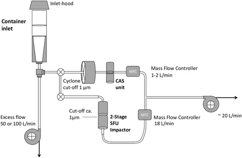
With preloaded two-stage stacked filter units (SFU; NILU Products AS), particles were collected on coarse and fine particle size fractions (Heidam, 1981). The SFU unit contained a coarse (8 μm pore size) filter and a fine (0.4 μm pore size) Nuclepore polycarbonate filter. The fine filter collected all particles <2 μm equivalent aerodynamic diameter (EAD; John et al., 1983). The coarse fraction was analysed but is not used because the focus of this study was on the sub-micrometre particles. The SFU was operated at a flow rate of 17 slpm downstream of an inlet at ambient conditions, which removed all particles (and cloud elements) above 10 µm EAD. The discrete SFU samples were collected for between 48 and 72 h. Figure 1 gives a schematic overview of the sampling arrangement. The flows of the CAS and SFU units were maintained and measured with mass-flow-controllers. The DC flow signals for CAS and SFU were recorded with a small HOBO data logger (Onset Computer Corp, Bourne, MA, USA).

Fig. 1. Schematic arrangement of samplers. CAS unit: 35 mm Nuclepore filter cassette. 2-Stage SFU impactor: 47 mm; open-faced 2-stage filter sampler with ∼1 µm cut size. Inset in the top-right shows a photo of the set-up of the CAS and SFU sampling lines.

2.2 Black carbon

Post-sampling determinations of the BC light absorption coefficient (σ_ap) were performed with a photometer at the Department of Meteorology, Stockholm University (MISU). Heintzenberg (1988) and Engström and Leck (2017) give technical details. To optimize the analytical conditions (increase the signal to noise ratio and provide filter area as optical blank) the PCMB Nuclepore filter surface was masked to 8 mm sampling diameter (0.5 cm² area) before sampling. The use of PCMB filters avoids high chemical blanks and is well suited for optical analyses.

The BC-photometer instrument used a 528 nm LED light source. A sensor behind the PCMB Nuclepore filter alternatively measured the diffusely transmitted light through the BC sample spot on the filter and the transmitted light through an unexposed part of the filter. The difference in intensity of transmitted light between exposed and unexposed filter surface was used to calculate the optical density (Od); σ_ap is defined as Od per metre of air column and is calculated by multiplying Od with the PCMB filter sample spot area and dividing by the volume of sampled air. BC mass concentrations were subsequently derived with a mass absorption efficiency coefficient of 10 m² g⁻¹ (Heintzenberg, 1982).

2.3. Inorganic compounds, MSA and oxalic acid

In order to minimize contamination of the filter substrates the PCMB Nuclepore filters were changed prior and after the exposure in a glove box (free from particles, sulphur dioxide and ammonia). After exposure, still inside the glove box, the filter substrates were extracted with 5 cm³ deionized water (18 MΩcm). For sufficient extraction the filter solutions were sonicated for 60 min. The extracts were thereafter analysed for major cations, anions and weak anions by chemically suppressed ion chromatography (IC, Dionex ICS-2000). The injection volume was 50 µdm³.

Quality checks of the IC-analyses were performed with both internal and external reference samples (Das et al., 2011). The average particulate sodium (Na⁺), ammonium (NH₄⁺), potassium (K⁺), magnesium (Mg²⁺), calcium (Ca²⁺), chloride (Cl⁻), oxalate (C₂O₄²⁻), nitrate (NO₃⁻), sulphate (SO₄²⁻), and methane sulphonate (MSA), blank concentrations were <5%, <3%, <1%, <0.2%, <0.3%, <6%, <0.1%, >0.2%, <0.2%, and 0% of the sample, respectively. Additional procedural information is given in Engström and Leck (2011). Non-sea-salt (nss)-SO₄²⁻ concentrations were calculated by using sodium concentrations and seawater composition taken from Stumm and Morgan (1981).

2.4 Polysaccharide markers

For the collection of airborne polysaccharides the two-stage SFU sampler was used. Field blanks were similar to the PCMB filter cassettes obtained by having no air drawn through the SFU sampler during the length of the sampling period. To avoid high chemical blank values all filter substrates were cleaned by ethanol and ultrapure water and then dried before use. Similar as in the protocol for the BC filter cassettes the SFU units were changed in a glove box both before and after sampling. After sampling the filters substrates (ambient and blank) were stored frozen at -80° prior to analyses. Polysaccharides were quantified after hydrolysis to their subunit monomer markers (monosaccharides) using hydrophilic lipophilic liquid chromatography (HILIC) coupled with tandem mass spectrometry (MS).

2.4.1. Hydrolyses

The SFU filter substrates were ultrasonically extracted with ultrapure water (Milli Q, resistivity 18 MΩ cm). Prior to extraction an amount of 100 pg of internal standard was added to the filter substrates to compensate for any error in quantification. Extracts were moved to a clean Pyrex glass container, baked for 2 h at 550 °C and then vacuum-dried by a rotary evaporator (RII, BUCHI, Switzerland). In order to hydrolyse the polysaccharides into their monosaccharide subunits, the residue in the evaporator was reconstituted in trifluoro acetic acid 4 M and incubated at 100 °C for 2 h. Subsequently, excessive acid was removed by vacuum evaporation and the residue was reconstructed in ultra-water and acetonitrile (20:80 v/v).

2.4.2. Determination

The following seven monosaccharides: pentoses: xylose (Xyl) and arabinose (Ara), hexoses: glucose/mannose (Glu/Man) and galactose (Gal) and deoxysugars: rhamnose (Rha) and fucose (Fuc) were targeted. With an ultra-high performance liquid chromatography (LC) system (Accela, Thermo Fisher Scientific) equipped with an amino propyl silica column and a guard column (Zorbax NH2 Agilent Technologies, Santa Clara, CA, USA) chromatographic separation of the hydrolysates, at isocratic condition, with a mobile phase mixture of acetonitrile and water (80:20, v/v) at a flow rate of 400 µl m⁻¹ was made possible.

The monosaccharides beside internal standards were identified and quantified employing an orthogonal triple-quadrupole mass spectrometer (TSQ Vantage, Thermo Fisher Scientific, Waltham, MA, USA) with a heated electrospray ionization (HESI) interface operating in negative mode. In order to obtain a sufficient selectivity and accuracy for trace level of the targeted monosaccharides they were quantified using an isotopic labelled internal standard technique in selected reaction monitoring mode with deprotonated monosaccharides as precursor ions ([M–H]⁻). Gao et al. (2011) give details on instrumental working parameters.

2.5 Positive matrix factorization

Receptor models are capable of estimating the contribution of the major pollution source categories with a level of accuracy that is in line with the needs of air quality management (Belis et al., 2015). PMF (Paatero, 1997) is a powerful receptor modelling method for the source attribution of airborne particulate matter (Hwang and Hopke, 2006). PMF has been successfully used to assess particle source contributions in the Arctic (Xie et al., 1999; Nguyen et al., 2013). The US EPA software PMF version 5.0 (Norris et al., 2014), short EPA-PMF5, is used in this study. PMF takes into account the estimated measurement uncertainty for each of the measured data values (Polissar et al., 1998). The estimation of measurement uncertainties provides a useful tool to decrease the weight of data that are missing or below detection limit. Further, PMF implements the non-negativity constraints on the factors in order to decrease the rotational freedom and to obtain more physically realistic factors.

The PMF model derives factor contributions and profiles through minimizing the objective function Q: (1) $$Q=\sum _{i=n}^n\sum _{j=1}^m{\left[\frac{x_{\mathit{ij}}-{\sum }_{k=1}^p{g}_{\mathit{ik}}{f}_{\mathit{kj}}}{u_{\mathit{ij}}}\right]}^2$$(1) where u_ij is the measurement uncertainty of concentration x_ij of the chemical compound/element denoted by index j in the sample denoted with index i; p is the number of sources that contribute to x_ij. It is then a least square problem to minimize Q with respect to the matrices of factor contributions, g, and factor profiles, f, with the constraint that each of the elements of g and f is to be non-negative.

Q is a critical parameter for PMF and two versions of Q are displayed in the EPA-PMF5 model runs (1) Q(true), the goodness-of-fit parameter calculated including all points; and (2) Q(robust), the goodness-of-fit parameter calculated excluding points not fit by the model, defined as samples for which the uncertainty-scaled residual is greater than four. Because Q(robust) is not influenced by points not fitted by PMF, it is typically used as the critical parameter for choosing the optimal run from the 20 base runs performed by EPA-PMF5. Q(robust) was inspected in the following to determine the reliability of the found solution.

In this study, the measurement uncertainty of each concentration value was estimated based on the relative error fraction of the analytical uncertainty, err_analyt, and the minimum detection limit (MDL) as: (2) $$u_{\mathit{ij}}=\sqrt{{\left({\mathit{err}}_{\mathrm{analyt}}·x_{\mathit{ij}}\right)}^2+{\left(0.5·\text{MDL}\right)}^2}$$(2)

Another aspect of weighting of individual data points is the handling of extreme values. The data were screened using the signal to noise ratio (S/N ratio) criteria described by Paatero and Hopke (2003), however no bad or weak variables were identified in the Mt. Zeppelin dataset. Missing values for a chemical compound were replaced by the corresponding median value of the entire time period together with an uncertainty of four times the median, as recommended in Brown et al. (2015). The scaled residuals in the PMF solution for the data points corresponding to the replaced missing values were clearly less than one, ensuring that the replacement did not influence the solution. Zero concentrations values in the dataset were replaced by the detection limit of the compound. One sample was excluded due to missing measurement of BC, leaving a total of 148 samples in 2015 for the PMF analysis. The mass of all particulate components in each sample was added to obtain the particulate mass of particles in sizes ≤1 μm in aerodynamic diameter (PM₁) of the sample. This underestimates the ambient PM₁ because only a small fraction of the organic carbon was identified in the chemical analysis (polysaccharides and oxalic acid). A mass-based approach for the particulate components was chosen, which, compared to a mole-based approach, has the advantage of attributing factors to certain mass fraction of total PM₁ in each sample, upon normalization of the concentrations with the measured total PM₁.

The optimal number of sources was determined to be eight based on examination of the scaled residual matrix and the Q values (Q(robust)=1074; Q(true)=1249). All 20 PMF base runs showed almost identical factor profiles and a very narrow range of Q(robust). The intra-run standard deviation of Q(robust) was 147, 0.026 and 12 for seven, eight and nine factors, respectively. With nine sources, an additional source that contributed less than 0.1% to total PM₁ was found. PMF has a tendency to suggest too many sources because this way the fit with the observed data can be improved. However, if only seven sources were chosen, oxalic acid (Oxal), a molecular tracer for aged secondary organic aerosol, was not associated with a distinct factor. The Q(robust) and Q(true) values for seven, eight and nine factors (each 20 base runs) are listed in Supporting Information Table S1. The expected Q value, Q_exp, for each solution was calculated as: (3) $$Q_{\exp }=\left(n·m\right)-\left(\left(p·n\right)+\left(p·m\right)\right)$$(3) where n is number of samples, m is number of chemical compounds (classified as strong in the PMF analysis) and p is the number of factors. When changes in Q become small with increasing factors, it can be indicative that there may be too many factors being fit (Brown et al., 2015). Q(true)/Q_exp is 1.813, 0.935 and 0.827 for seven, eight and nine factors. The small change from eight to nine factors indicates that eight factors is the optimal solution. In the selected base run of the three solutions, the ratio Q(true)/Q_exp for each sample is listed in Supporting Information Table S2 and the ratio Q(true)/Q_exp for each chemical compound is listed in Supporting Information Table S3. For each chemical compound, Q(true)/Q_exp corresponds to the sum of the squares of the scaled residuals, divided by the overall Q_exp divided by the number of chemical compounds. Inspection of Q(true)/Q_exp per compound shows that the solution with eight factors greatly reduces the residuals for Na⁺ and sea-salt sulphate (ss-SO₄²⁻) compared to the seven-factor solution. The nine-factor solution only slightly changes the residuals for most compounds compared to the eight-factor solution.

The parameter FPEAK is used to control the rotational freedom of the factors found in the base run solution (Paatero et al., 2002). For the eight-factor solution, FPEAK runs with values between −1.0 and 1.0 were examined, giving Q(robust) range of 1158 − 1560. Q(robust) was very stable in the range of FPEAK values between −0.1 and 0.1. The FPEAK value was therefore set equal to 0. The FPEAK runs did not reveal significantly different factor profiles.

Variability due to chemical transformations or process changes acting on the particle composition can cause significant differences in the factor profiles among PMF runs. The variability of the source profiles obtained from the PMF analysis was estimated using a block bootstrap technique implemented in EPA-PMF5. The bootstrap analysis helps to measure the variability in the source profile with respect to the variability in the input concentration data. It is important to note that variability and uncertainty are not equivalent. Uncertainty associated with a source profile can only be constructed if the underlying uncertainty distribution is known. Thus, running multiple block bootstrap runs on the same source profile is necessary to construct source profile uncertainties. Bootstrap (BS) data sets are constructed by sampling, with replacement, from the original input data set. BS error intervals include effects from random errors and partially include effects from rotational ambiguity. BS determined errors are generally robust and not influenced by the user-specific sample uncertainties. In this study, 200 BS runs were performed.

2.6 Potential source distribution

For every hour of the present study 3D trajectories have been calculated arriving at the height of the mountain station. The trajectories have been calculated backward for up to 10 days using the HYSPLIT4 model (Draxler and Rolph, 2003; Stein et al., 2015) with meteorological data from the Global Data Assimilation System with one-degree resolution (GDAS1). The meteorological fields were downloaded from the server at Air Resources Laboratory (ARL), NOAA (http://ready.arl.noaa.gov), where more information about the GDAS dataset can be found. Note, that the mean wind speed at Mt. Zeppelin is ca. 6 m s⁻¹, which means that the first time step of a trajectory corresponds to 20 km, limiting the value of individual trajectories for a closer analysis at Svalbard (horizontal distance between Ny-Ålesund port and the Zeppelin observatory is roughly 3 km). Another limitation for using back trajectories in the analysis of local air pollution transport lies in the fact that the HYSPLIT4 model can only represent the Svalbard topography in highly smoothed form.

Heintzenberg et al. (2011) presented a method to extrapolate aerosol measurements taken at one station to a larger area by means of back trajectories that was later developed further and applied to several regional aerosol source investigations (Heintzenberg et al., 2013; Heintzenberg et al., 2015; Heintzenberg et al., 2017). PSDs were derived from this method by distributing measured hourly aerosol parameters like total number concentrations along corresponding hourly back trajectories from the measuring site up to 10 days back in time over a gridded map about the receptor site. Whenever a trajectory passes over a geo-cell of the map the respective aerosol parameter is accumulated for a temporal average in the cell. Geo-cell averages are then calculated over whole experiments, seasons or sample periods. The method was validated with aerosol data measured near distant trajectory points in Heintzenberg et al. (2011).

For the present study PSDs were constructed to identify the potential aerosol source regions related to the PMF factors. For that purpose the values of the PMF-factors were distributed along hourly back trajectories during all sample periods. For each PMF-factor one average PSD was established by averaging over all trajectories of the studied sample periods.

2.7 Auxiliary measurements and data (post-analysis)

Auxiliary measurements at the Zeppelin observatory were used: (1) wind speed and wind direction as hourly averages; (2) trace metal concentrations in weekly PM₁₀ (PM ≤ 10 μm in aerodynamic diameter) samples and (3) major inorganic component concentrations in PM₁₀ in 1-day filter samples (3-filter-pack; Aas et al., 2016). Concentration of trace elements in PM₁₀ collected with a high-volume sampler were determined by Inductively Coupled Plasma Mass Spectrometry (ICP-MS) including vanadium (V), chromium (Cr), manganese (Mn), nickel (Ni), copper (Cu), zinc (Zn), arsenic (As), selenium (Se), cadmium (Cd) and lead (Pb). The sampling was performed by exposure of the filter for two consecutive days (48 h) once per week. These measurements are part of the ‘Cooperative Programme for Monitoring and Evaluation of the Long-range Transmission of Air Pollutants in Europe’ (EMEP) monitoring program at the Zeppelin observatory (Berg et al., 2008; EMEP, 2014; Aas et al., 2016) by the Norwegian Institute for Air Research (NILU). Data sets were obtained from the EBAS database (http://ebas.nilu.no).

Soil samples near the settlement of Ny-Ålesund were taken in the SHIPMATE (Ship Traffic Particulate Matter Emissions) project in June 2014 (López-Aparicio et al., 2016). A complete extraction of soil samples and subsequent metal analysis were carried out at NILU and the average metal concentrations in 15 soil samples are reported in López-Aparicio et al. (2016). The concentrations of crustal V, Ni, Mn and Cr in PM₁₀ samples were calculated from the mass ratios of these elements to aluminium (Al) in the soil samples. The non-crustal (nc) V, nc-Ni, nc-Mn and nc-Cr were obtained by subtracting crustal V, Ni, Mn and Cr from the total V, Ni, Mn and Cr in the PM10 samples at Mt. Zeppelin. These non-crustal metals and the ratio nc-V/nc-Ni were used as indicators for fossil-fuel combustion and ship emissions in the post-analysis of PMF factors.

Daily passenger data from ships arriving in the port of Ny-Ålesund based on port calls recorded by the harbour master of Kings Bay AS Company were used in this study as a proxy for shipping activity and therefore potential local pollution. The majority of anchoring ships are tourist ships that cruised in the Kongsfjord for a few hours before or after visiting Ny-Ålesund. Emission data of air pollutants from ship traffic on the Barents Sea and Norwegian Sea were additionally obtained from the Norwegian Coastal Administration to complement the information from port calls (https://havbase.no/). Monthly shipping emission totals were estimated with the model developed by DNV-GL, which makes use of ship position and identification data recorded with the Automatic Identification System (AIS) in order to estimate fuel consumption and emissions.

In an earlier study on aerosol formation in the inner Arctic information on pack ice extent under the air masses reaching the sampling points proved crucial (Heintzenberg et al., 2015). Also, the fact that the Svalbard region experiences large seasonal changes in pack ice cover does affect marine traffic in the region and can be expected to have strong effects on near-surface aerosol emissions. Therefore, daily sea ice concentrations from Nimbus-7 SMMR and DMSP SSM/I-SSMIS passive microwave data were taken from the NSIDC database (https://nsidc.org/data). Around the pole a roughly circular gap in ice data is caused by the inclination of satellite orbits. To each hourly position and data of the back trajectories (Section 2.6) the ice information was added. On average the closest ice information from the ice maps was about 12 km off any trajectory point. Monthly maps of total ice concentrations were constructed for the interpretation of the aerosol data.

3. Results

3.1 Results of the chemical analyses

Table 1 summarizes measured mean, median and maximum concentrations of selected aerosol components at the Zeppelin observatory during the study period (year 2015). The annual mean concentration of BC was 18 ± 8.5 ng m⁻³ (±1 SD), which is lower than the previous reported annual mean concentration of 46 ± 19 ng m⁻³ by Yttri et al. (2014) for a 1-year period during 2008 − 2009 and 39 ng m⁻³ by Eleftheriadis et al. (2009) for the time period 1998 − 2007 at the Zeppelin observatory. Yttri et al. (2014) used data from a Particle Soot Absorption Photometer (PSAP) operated with an almost identical light source wavelength (522 nm) as in this study (528 nm) but applied a lower mass absorption efficiency coefficient of 5.7 m² g⁻¹ in their calculation of BC equivalent mass concentrations than in this study (10 m² g⁻¹). This difference in the assumption of mass absorption efficiency coefficient can explain the lower annual mean BC concentrations deduced from the optical measurements of the present study. This study’s seasonal variation of BC is similar to previous studies with relatively increased average concentrations of 28 ± 30 ng m⁻³ in winter (October to April) compared to average concentrations (11 ± 19 ng m⁻³) in summer (May to September). Note that the winter concentration average in this study includes data from sampling during October to December 2014.

Table 1. Concentration of BC and selected cations and anions (ng m⁻³) at the Zeppelin observatory during the study period (01 January 2015 to 31 December 2015).

Compound	BC	MSA	NH4^+	NO3^−	Na^+	SO4^2− (tot)	nss- SO4^2-	K^+ (tot)	nss- K^+	Ca^2+
Mean (ng m^–3)	18	5	78	10	49	289	276	3.5	2.0	10
Median (ng m^–3)	9.4	0.5	48	8.4	34	149	127	1.8	0.35	7.6
Maximum (ng m^–3)	147	69	478	30	280	1805	1739	40	40	57

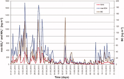
Sulphate and ammonium are major components of the sub-micrometre aerosol at Mt. Zeppelin. The nss-SO₄²⁻ concentrations in 2015 ranged from 7.7 to 1740 ng m⁻³, with a mean of 276 ng m⁻³. The NH₄⁺ concentrations ranged from 0.3 to 478 ng m⁻³, with a mean of 78 ng m⁻³. Concentrations of nss-SO₄²⁻ and NH₄⁺ were increased during the haze period, in particular between January and April (Fig. 2). This is indicative for long-range transport of pollution during Arctic haze in winter and spring. Concentrations of nss-SO₄²⁻ and BC are correlated to some extent for the entire year (R²=0.62, N = 148 samples). The correlation is higher in the period January to April (R²=0.72, N = 47 samples), but very low in the period May to September (R²=0.25, N = 65 samples). In summer (May to September) nss-SO₄²⁻ concentrations are much lower than in winter (by an average factor of five compared to the haze period), with a peak in July and early August. In summer, inner-Arctic ship emissions and oxidation of DMS from marine phytoplankton in seawater mainly contribute to sulphate. Aerosol NH₄⁺ appears to be in mainly the form of sulphates as nitrate concentrations are rather low (mean NO₃⁻ concentration is 10 ng m⁻³). The molar ratio of NH₄⁺ to nss-SO₄²⁻ in all samples has a mean value of 2.11, indicating ammonium sulphate. The median value, upper quartile and lower quartile of the molar ratio are 1.76, 3.12 and 1.29, respectively. From May to September, 83% of the samples have a molar ratio equal or above 2.0, corresponding to a predominant composition of ammonium sulphate. In winter and autumn, nss-SO₄²⁻ is only partly neutralized by ammonium and most samples exhibit a molar ratio equal or below 1.5.

Fig. 2. Concentrations of NH₄⁺ (red line), nss-SO₄²⁻ (blue line), and BC (brown line, second y-axis) measured during 2015 at the Zeppelin observatory.

Calculation of the total PM₁ as the summation of all measured compound concentrations in the sampled particulate matter during 2015 results in range 31–2600 ng m⁻³ with a mean of 458 ng m⁻³ (median: 296 ng m⁻³) at Zeppelin observatory. The mean concentration of the sum of determined polysaccharide markers was 0.48 ng m⁻³. The analysed polysaccharide markers represent only a fraction of the primary saccharides in the ambient aerosol. In a recent study by Fu et al. (2013) the speciation of the organic fraction in marine aerosol from the Arctic Ocean showed primary saccharides (including sugar alcohols) in the range 0.9–112 ng m⁻³.

PM₁ from summation does not include the complete sea salt because chlorine (Cl⁻) has been, similar as in the study by Leck et al. (2002), depleted to a large extent in the acidic sub-micrometre aerosol before arrival at the receptor site. To derive the actual sea salt concentration, the ratio of Cl⁻/Na⁺ of 1.33 derived from PM₁₀ from 1-day air 3-filter-pack samples (EBAS: http://ebas.nilu.no) together with the sea salt formula: [sea salt] = 1.8 [Cl⁻] (Malm et al., 2007) was used. A mean sea salt concentration in PM₁ of 112 ng m⁻³ (median: 81.8 ng m⁻³) was obtained.

Total organic matter can only be derived indirectly because organic carbon (OC) was not determined in the samples. Zhan et al. (2014) reported EC/OC ratios in aerosol measured in the settlement of Ny-Ålesund in the range 0.0076–0.28 (median: 0.04) during summer. To derive total organic matter (OM) in PM₁ the measured BC concentration (used here instead of EC concentration) was translated by using an EC/OC ratio of 0.04 (Zhan et al., 2014) and [OM] = 1.8 [OC] (Malm et al., 2007). This approach gave a mean OC and OM concentration of 442 ng C m⁻³ and 796 ng m⁻³, respectively. The estimated OC is close to the reported mean OC concentration in marine aerosols from Arctic Ocean in summer (i.e. 560 ng C m⁻³, range: 110–2930 ng C m⁻³; Fu et al., 2013).

The chemically reconstructed mass derived from the procedures described above and in Malm et al. (2007) gave a mean PM₁ of 1320 ng m⁻³ (median: 699 ng m⁻³), composed of organic matter, sulphate (as (NH₄)₂SO₄), sea salt, EC (assumed to be the same as BC) and nitrate (as NH₄NO₃) with respective contributions of 60%, 29%, 8.5%, 1.3% and 1.0% to the total mass. Soil dust is assumed to be mainly in the coarse particulate mass and therefore was neglected in the chemical reconstruction. Studies on the size distribution of atmospheric trace elements at Dye 3 in Greenland have shown that for atmospheric trace elements associated with soil dust most of the mass occurs in particle sizes above 1.0 μm (Hillamo et al., 1993; Jaffrezo et al., 1993).

The mean total PM₁ mass derived from aerosol mobility size distributions obtained from measurements by Differential Mobility Particle Sizer (DMPS) during 2015 at the Mt. Zeppelin observatory is 640 ng m⁻³, based on an estimated dry particle density of 1680 kg m⁻³. The annual mean PM₁ from aerosol mobility size distributions indicates that the chemical analyses in our study accounted for 72% of the total sub-micrometre mass.

3.2 Results from PMF analysis of PM₁

The PMF solution that best represented the temporal variability of the analysed components of PM₁ identified eight sources of the sub-micrometre aerosol mass: four natural, two anthropogenic and two secondary. The four natural sources include three primary sources (i.e. sea spray and two types of marine gel sources) and one secondary natural source of marine biogenic aerosol. The two anthropogenic sources consisted of biomass burning and a mixed combustion source. The two identified secondary sources from the regional background are secondary sulphate and secondary nitrate aerosol, which together constitute 61% of the particulate mass on annual average. Table 2 summarizes the PMF factors, their relative and absolute contribution to PM₁, together with the associated uncertainty of the contribution determined from the BS analysis. The average chemical composition of the eight factors is listed in Supporting Information Table S4.

Table 2. Source attribution from the PMF analysis to the annual mean PM₁ of 2015.

PMF factor	Source interpretation	Rel. PM1 contribution [%]	PM1 contribution [ng m^−3]	5th percentile [ng m^−3]	95th percentile [ng m^−3]
1	Regional background secondary sulphate	55.7	255.0	186.6	298.3
2	Sea spray	16.6	76.1	53.1	99.1
3	Marine gel type 1	0.4	2.0	0.4	7.0
4	Biomass burning	15.0	68.7	21.6	155.5
5	Regional background secondary nitrate	5.8	26.7	17.6	46.9
6	Secondary marine biogenic	4.5	20.4	13.0	45.6
7	Mixed combustion	1.6	7.4	1.8	22.6
8	Marine gel type 2	0.3	1.4	0.6	11.5

PM₁ concentration attributed to each PMF factor and associated uncertainty, given as 5th and 95th percentile of the BS runs.

3.2.1 Factor 1: Regional background secondary sulphate

The most important PM₁ component on annual basis is ammonium sulphate. NH₄⁺ and nss-SO₄²⁻ are the dominant constituents of factor 1 (Fig. 3a), classifying this factor as secondary aerosol, abundant in the regional background, with sulphur having both natural and anthropogenic sources. Ammonium sulphate appears to be a common component in the ‘accumulation mode’ (between 70 and 500 nm diameter) of aerosols with natural sources (Leck and Persson, 1996b; Bigg and Leck, 2001), often mixed with methane sulphonate (MSA) deriving from the oxidation of DMS. In remote marine environments, gaseous ammonia (NH₃) mainly originates from the ocean, from the bacterial remineralization of particulate organic matter (Carpenter et al., 2012). Coastal seabird colonies were found to be an important source of NH₃ in the summertime Arctic (Wentworth et al., 2016), although the temporal and spatial variability of this source is highly uncertain. The biological activity within sea ice has also been suggested as NH₃ source found in Antarctic ice (Thomas and Dieckmann, 2002). Long-range transport of NH₃ from animal husbandry and industrial sources at lower latitudes probably has a limited influence in summer, but might contribute substantially to the ammonium sulphate aerosol during winter.

Fig. 3. Factor profiles from the PMF base run: (a) Factor 1 [Regional background secondary sulphate], (b) Factor 2 [Sea spray], (c) Factor 3 [Marine gel type 1], (d) Factor 4 [Biomass burning], (e) Factor 5 [Regional background secondary nitrate], (f) Factor 6 [Secondary biogenic marine], (g) Factor 7 [Mixed combustion], and (h) Factor 8 [Marine gel type 2]. Polysaccharide markers (Xyl, Ara, Rha, Fuc, GluMa and Gal) are displayed as orange bars and refer to the second y-axis. Error bars of the compound/element concentrations in the factor profile indicate the uncertainty range from the bootstrapping with 5th percentile as lower limit and 95th percentile as upper limit.

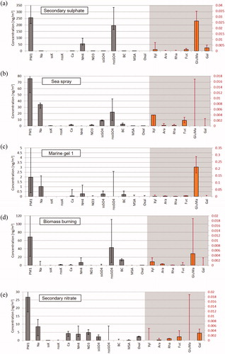
3.2.2 Factor 2: Sea spray

The sea spray factor is clearly dominated by Na⁺, Ca²⁺, sea salt (ss)-K⁺ (about 75% apportioned to this factor) and ss-SO₄²⁻ (Fig. 3b). A contribution from ship traffic or another combustion source to this factor is evident. Mixing of the sea salt aerosol with polluted air masses is significant, with presence of BC, nss-SO₄²⁻ and NO₃⁻. Nitrate is the oxidation product of nitrogen oxides (NO_X) from combustion sources or metal smelters. Nguyen et al. (2013) also identified a contribution from anthropogenic pollution to the marine aerosol factor at station Nord in North East Greenland.

Sea salt is present throughout the whole year with the exception of late summer. Increased wind speeds are expected to increase white cap of breaking waves and lead to injection of more sea salt droplets into air (Monahan and O’Muircheartaigh, 1986). Other parameters such as sea surface temperature (Mårtensson et al., 2003) and sea ice cover (Nilsson et al., 2001) are known to influence the sea salt particle emissions. Peak contributions from the sea spray factor coincide with high wind speed measured at Mt. Zeppelin (Supporting Information Fig. S2).

3.2.3 Factor 3: Marine gel type 1

The compounds contributing to the third factor (Fig. 3c) included Na⁺, Ca²⁺, and ss-SO₄²⁻, indicating seawater origin. This profile was identified as marine gel particles due to the presence of Glu/Man and other monosaccharides (Rha and Fuc), which despite being present in very small quantities, were mainly apportioned to this factor and showed small variability of the apportioned concentrations. The Glu/Man monosaccharides (related to structural polysaccharides, which constitute the cellular materials of phytoplankton) and the monosaccharides Rha and Fuc (exudates derived from phytoplankton and/or non-photosynthetic microbial bacteria) have been observed to be abundant in the particulate organic matter (POM) of samples collected in open water in the central Arctic Ocean (Gao et al., 2012).

The indicated seawater origin of factor 3 shows in the presence of Ca²⁺. The interpretation of the likely source of Ca²⁺ is however ambiguous. On one hand, its presence seems consistent with the observed enrichment of Ca²⁺ in sub-micrometre sea spray particles generated using a sea spray chamber filled with artificial seawater with absence of POM (Salter et al., 2016). On the other hand, Ca²⁺ is also known to provide bridges between adjacent or different polysaccharide chains in the marine gel 3D structures (Chin et al., 1998). The ratio Ca²⁺/Na⁺ in seawater was used to calculate nss-Ca²⁺ in the sub-micrometre particles from Mt. Zeppelin observatory. The average ratio of nss-Ca²⁺ to Ca²⁺ in the sub-micrometre particles was 0.67 ± 0.31. The study of Leck and Svensson (2015) attributed observed significant enrichment of Ca²⁺ in a number of ambient aerosol samples collected over the central Arctic Ocean during summer to organic matter in the form of marine gels. BC and, although uncertain, nss-SO₄²⁻ is found in this factor, suggesting some mixing with polluted air masses before arrival at the receptor site. The increasing inner-Arctic shipping activities including fishery and sightseeing cruises (Hagen et al., 2012; Ødemark et al. 2012) could explain BC and nss-SO₄²⁻ in this marine source. The marine gel factor was found to contribute only 0.4% to PM₁ on an annual basis, but aerosol samples in September-November showed PM₁ contributions of up to 12%. PMF identified a second marine gel factor; therefore, this factor is referred to as marine gel type 1 in the following.

3.2.4 Factor 4: Biomass burning

The typically chosen markers of biomass burning in PMF analysis are levoglucosan (a combustion product of cellulose at temperature above 300 °C) and K⁺. Levoglucosan was not included in the chemical analysis of this study, but fortunately, non-sea salt potassium (nss-K⁺), which is a well-known qualitative marker for biomass burning (Cachier et al., 1995; Frossard et al., 2011; Pachon et al., 2013). In the Arctic wind-blown soil dust can also be a source of potassium. Pio et al. (2008) estimated potassium related to biomass burning, K⁺_bb, as the fraction of K⁺ not associated with sea salt and soil dust particles by: (4) $${\mathrm{K}}_{\text{bb}}^{+}={\mathrm{K}}^{+}-0.036{\text{Na}}^{+}-0.12\left(\text{nss}-{\text{Ca}}^{2+}-{\text{Ca}}_{\text{bb}}^{2+}\right)$$(4)

In this expression, nss-Ca²⁺ refers to non-sea salt calcium and Ca²⁺_bb refers to Ca emitted in biomass burning. The latter is derived from a mass ratio of ten for K⁺_bb/Ca²⁺_bb. Biomass burning K⁺_bb was highly correlated with nss-K⁺ (R²=0.90) in PM₁ at Mt. Zeppelin.

The biomass-burning factor included BC (75% of compound apportioned to biomass burning) and NH₄⁺ and, with substantial uncertainty in the apportionment, nss-SO₄²⁻ (Fig. 3d). The reason for finding sulphate associated with the biomass burning could be the mixing with fossil fuel combustion aerosol during the haze period, which was not possible to separate from the biomass burning factor by PMF. Thus, it cannot be ruled out that pollution from fossil combustion sources contributed to the biomass-burning factor in winter.

Biomass burning, although identified by a single fingerprint in the PMF analysis, likely has different seasonal origins and sources. In winter, residential heating could be the main source whereas during summer, the biomass burning plumes from wildfires could be prevalent. A one-year time series from March 2008 to March 2009 of levoglucosan measurements at Zeppelin observatory revealed elevated mean concentrations of levoglucosan in winter, about a factor of ten higher than in summer (Yttri et al., 2014). Episodes of elevated levoglucosan concentration lasting up to 6 days were found to be more frequent in winter than in summer (Yttri et al., 2014). Modelling with the Lagrangian particle dispersion model FLEXPART (Stohl et al., 2005) captured the seasonal pattern of the observed levoglucosan time series, predicting a period of increased impact from residential wood burning emissions between mid-November and March (Yttri et al., 2014). The study provides an estimated upper limit of 31%–45% for the wintertime contribution of biomass burning to BC, which supports the interpretation that factor 4 in our PMF analysis is partly mixed with fossil fuel combustion aerosol in winter.

3.2.5 Factor 5: Regional background secondary nitrate

Factor 5 is characterised by the marker oxalate (C₂O₄²⁻), referred to as Oxal, and is composed of secondary inorganic ions NH₄⁺ and NO₃⁻ mixed with the sea salt constituents Na⁺, Ca²⁺, and ss-SO₄²⁻ (Fig. 3e). The factor includes a high concentration of nitrate. Nitrate forms in the atmosphere through the oxidation of NO_X, which could come from industrial combustion processes and emissions from ship traffic. Factor 5 is classified as secondary nitrate aerosol abundant in the regional background. Secondary nitrate replaces secondary sulphate as the predominant PM₁ source in late summer and autumn. It is known that lower temperature and higher humidity favour the formation of secondary nitrate particles (Seinfeld and Pandis, 2006). NO₃⁻ may originate from the replacement of Cl⁻ in sea-salt particles through the formation of sodium nitrate (Brimblecombe and Clegg, 1988), supported by the sea salt constituents associated with this factor.

Observations show that dicarboxylic acids like oxalic acid are commonly found in the organic fraction of secondary aerosol in marine environments (e.g. Mochida et al., 2003). Oxal is one of the main identified single organic particle mass components. Oxal forms in cloud processing or chemical ageing of VOCs from biogenic and anthropogenic sources. In the marine atmosphere, the aqueous phase oxidation of glyoxal in clouds is an important pathway leading to particulate Oxal. Glyoxal results from the gas-phase oxidation of acetaldehyde and toluene and the oxidation of glycolaldehyde (Warneck, 2003), for which methylvinylketone (MVK) is the most important precursor. MVK is one of the main isoprene oxidation products. As shown by Lim et al. (2005) this pathway links isoprene, emitted from trees and to a smaller extent from oceanic phytoplankton (e.g. Spracklen et al., 2008), and oxalic acid. Chang et al. (2011) previously identified in the PMF analysis of the aerosol measurements using an aerosol mass spectrometer (AMS) during the Arctic Summer Cloud Ocean Study (ASCOS) expedition an aged organic component in a PMF-factor that they interpreted as continental source, consistent with aerosol that has been extensively oxidised in the atmosphere with long residence time (Ng et al., 2010).

3.2.6 Factor 6: Secondary marine biogenic

Methane sulphonate (MSA) is typically present in ambient marine particles; thus making it a suitable tracer for secondary marine biogenic aerosol. About 95% of MSA was apportioned to the secondary marine biogenic factor (Fig. 3f). This factor is present during summer, containing MSA and sulphate, mixed with other secondary inorganic aerosol components such as NH₄⁺ and to a smaller extent NO₃⁻. It contributes 4.5% to the annual averaged PM₁. The presence of NH₄⁺ in the secondary biogenic aerosol could indicate that the particles contain partly or fully neutralized ammonium sulphates and methane sulphonate. Only a small fraction of the measured monosaccharides, representing primary emitted marine gels, were apportioned to the marine biogenic aerosol, with Fuc being the highest (13% of the compound).

Oceanic emission of DMS is the only known source of particulate MSA. In the Svalbard region, the melting ice edge gives rise to a spring bloom of phytoplankton (April to June), leading to the release of DMS to the atmosphere from the uppermost ocean layer as observable in the corresponding high DMS mixing ratios at Zeppelin observatory (Park et al., 2013).The gas-phase oxidation of DMS leads to particulate MSA and sulphate upon condensation and/or heterogeneous uptake on particles. Thus MSA and nss-SO₄²⁻ from biogenic sources, with minimum anthropogenic influence, are expected with constant ratio in the aerosol. The non-sea salt sulphate in the secondary marine biogenic factor showed high uncertainty in its apportionment. In order to estimate the MSA/nss-SO₄²⁻ mole ratio of the factor, bootstrapping analysis with displacement (BS-DISP) of nss-SO₄²⁻ was used. The average MSA/nss-SO₄²⁻ molar ratio of the secondary marine biogenic factor was 0.36 with a lower limit of 0.19 determined by BS-DISP. It was not possible to establish an upper limit due to the entirely uncertain contribution from nss-SO₄²⁻ to the factor.

The found average MSA/nss-SO₄²⁻ molar ratio lies within the range of values calculated from a box model for conditions of the AOE-96 expedition using different DMS chemistry schemes (0.28–0.39, mean 0.32; Karl et al., 2007). It is also similar to the molar ratio of 0.28 reported by Heintzenberg and Leck (1994) in the Arctic summer sub-micrometre aerosol at Spitsbergen, but higher than the MSA/nss-SO₄²⁻ molar ratio attributed to marine biogenic sources (0.22) from sub-micrometre filter measurements during IAOE-91 (Leck and Persson, 1996b). The MSA/nss-SO₄²⁻ molar ratio is partly controlled by temperature as a consequence of the involved temperature-dependent gas-phase reactions of DMS.

3.2.7 Factor 7: Mixed combustion

The mixed combustion source with common presence of BC, nss-SO₄²⁻ and NO₃⁻ (Fig. 3g) is mainly active in early summer, during the end of the haze period, and in autumn. The mixed combustion source could be related to inner-Arctic activities or to long-range transported pollution from continental sources in the high latitudes of Eurasia or North America. According to Nguyen et al. (2013), 80%−98% of BC at station Nord in Greenland are apportioned to anthropogenic sources, while the remaining fraction has been associated with marine and soil dust sources. In the PMF analysis, only 2.2% of BC was associated with the mixed combustion source.

The mixed combustion source accounts for only 1.6% of the annual averaged PM₁, however its impact has likely been underestimated due to missing markers for anthropogenic organic carbon (OC) in the chemical analysis of the PM₁ samples in this study. Interestingly, about 80%−90% of galactose (Gal) was apportioned to the mixed combustion source, together with glucose and mannose (Glu/Man; concentration average ca. 0.1 ng m⁻³). In conjunction with the other compounds associated with the factor, glucose is a marker for combustion sources. Glucose and mannose have been detected in smoke from wood combustion (‘wood smoke’; Engling et al., 2006). The presence of Glu/Man in fine mode particles has been related to the combustion of biomass (Nolte et al., 2001), whilst glucose in coarse mode particles is most probably from primary biological sources such as plant debris and pollen (Tominaga et al., 2011). Galactose has been detected in particles from soil biota (Simoneit et al., 2004), which would confirm the continental origin of this factor.

The finding of primary saccharide associated with combustion sources is in concert with the high sub-micrometre mass contribution of Glu/Man (78%) collected during the ASCOS expedition in an episode when the boundary layer air had come from the Canadian Archipelago (Leck et al., 2013). Based on the Glu/Man fingerprint Leck et al. (2013) concluded that the boundary layer over the central Arctic Ocean was influenced by continental combustion sources.

3.2.8 Factor 8: Marine gel type 2

PMF isolated a second marine gel factor, referred to as marine gel type 2 in the following, dominated by the monosaccharide Xyl (85% of compound apportioned to marine gel type 2) and Ca²⁺ (Fig. 3h). The attribution of NH₄⁺ and Oxal (0.7% and 0.6% of compound apportioned, respectively) to this factor is highly uncertain but their abundance in the background could indicate relatively long travel time of the marine gel particles before reaching Zeppelin observatory. Marine gel type 2 occurred infrequently during autumn and winter; its contribution to annual average PM₁ was limited (0.3%).

As discussed with marine gel type 1, the presence of Ca²⁺ indicates seawater origin. As pointed out above, divalent ions (Ca²⁺ and Mg²⁺) are known to provide bridges between adjacent or different polysaccharide chains responsible for the gel-like consistency of the marine gels (Chin et al., 1998). Leck and Bigg (2010) and Hamacher-Barth et al. (2016) in using high resolution X-ray spectrometer both found that calcium is a major element in marine gel particle samples collected at Cape Grim and during the ASCOS expedition. Near-absence of sodium in factor 8 suggests that the marine gels were not attached to sea salt, similar as observed by Leck and Bigg (2010) in the Cape Grim samples.

3.2.9 Summary of the PMF results

According to the PMF solution, black carbon on annual average was mainly (by 75%) associated with biomass burning (factor 4) and to a smaller extent (by 17%) with sea spray (factor 2). The contribution from the sea spray source indicates mixing of the sea spray aerosol with anthropogenic pollution, for example from shipping emissions, before arrival at the receptor site. The contribution from the identified mixed combustion source (factor 7) to BC was only 2.2%.

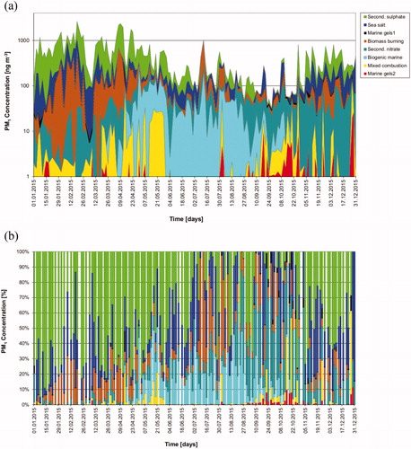
The source contributions from the eight factors to PM₁ have a distinctive seasonality, as shown in Fig. 4. Secondary sulphate (factor 1) is the predominant aerosol constituent in the Arctic haze period (November to April). The biomass-burning source has a high contribution (10%–30%) from January to April and then peaks again in July. Sea spray contributes in both winter and summer and is the third largest PM₁ constituent on annual basis. During spring and summer (April-August), secondary marine biogenic (factor 6), identified by the marker MSA, becomes important and reaches a contribution of up to 50% in some samples. Secondary nitrate (factor 5) mainly contributes towards the end of summer and in autumn. The mixed combustion source (factor 7) occasionally contributed up to 55% in spring and autumn. The primary marine gel sources (factor 3 and 8) are active from September to December, with contributions of a few percent up to 20%. Figure 4 shows the factor profiles; the BS uncertainty results for the eight factors are summarized in Supporting Information Fig. S1.

Fig. 4. Seasonal variation of the factor contributions to PM₁ at Mt. Zeppelin according to the PMF 8-factor solution for the samples in 2015: (a) cumulative source contribution of PMF factors to PM₁ concentrations and (b) percentage source contribution of PMF factors to PM₁ concentrations. Note the logarithmic scale of the y-axis in figure part (a). White vertical lines in figure part (b) represent sampling gaps.

4. Source regions and processes

4.1 Potential source regions for PMF factors

For the understanding of potential aerosol source regions related to the PMF-factors five-day back trajectories during each hour of aerosol sampling were utilized. The results in Fig. 3 show a rather broad distribution of the factor contributions, i.e. the values of the individual PMF-factors scatter over more than one order of magnitude during the year, probably because naturally every sample covers varying air masses during its passage to the receptor site. Thus, in order to sharpen the trajectory analysis only trajectories connected with factor values larger than the 99th percentile of each PMF factor were utilized. Per PMF-factor this sharpening left between 94 and 122 trajectory hours. The related factor values were then distributed along the trajectories related to respective samples, and in each geo-cell the respective factor values were averaged in order to obtain geographic PSD maps for each PMF factor. On the geographic maps in Fig. 5 only geo-cells are shown with at least 60 trajectory hits and the colour scales of the eight maps in Fig. 5 were adjusted to the maximum values of each PMF-factor. Average and median PMF-weighed trajectory heights related to the data in Fig. 5 are drawn in Fig. 6.

Fig. 5. Maps of potential source distributions of the aerosol sources identified by the 8-factor PMF solution and 5-day back trajectories. Top row: Factors 1–4; bottom row: Factors 5–8. The colour scales of the individual maps are adjusted to the peak values of the respective PMF-factors: (a) Factor 1 [Regional background secondary sulphate], (b) Factor 2 [Sea spray], (c) Factor 3 [Marine gel type 1], (d) Factor 4 [Biomass burning], (e) Factor 5 [Regional background secondary nitrate], (f) Factor 6 [Secondary biogenic marine], (g) Factor 7 [Mixed combustion], and (h) Factor 8 [Marine gel type 2]. Only geo-cells with ≥60 trajectory hits per cell are shown. The red symbol indicates the North Pole.

Fig. 6. Left: Average PMF-weighted trajectory heights during 240 h before air mass arrival at the receptor site at 474 m a.s.l., related to the maps in Fig. 5; right: PMF-weighted 50 percentiles trajectory heights.

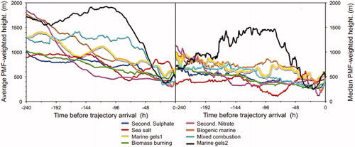
The highest average values of PMF factor 1 (regional background secondary sulphate) are connected with a rather narrow air mass pathway from the continental source region between the Ural and the Kola Peninsula (Fig. 5a). Most frequent trajectory heights on this pathway are above 500 m (cf. Fig. 6). The Kola Peninsula and other parts of northern Russia have Cu and Ni and other non-ferrous metal producing industries, which are strong emitters of sulphur dioxide (SO₂) and NO_X (Hole et al., 2006). The conurbation of Murmansk, a highly populated metropolitan area and maritime port, also contributes to the polluted air from the Kola Peninsula (Law and Stohl, 2007).

Map two (Fig. 5b) relates to the sea spray aerosol source. High average PMF-factor values are located over the open ocean between Fram Strait and Jan Mayen with a secondary area over the Kara Sea. The trajectories related to this factor most frequently stay below 500 m height for most of their 10-day length.

Maps for factor 3 (Fig. 5c) and factor 8 (Fig. 5h) concern marine gels of type 1 and 2, respectively. They both reach from the Fram Strait between Greenland and Svalbard and the open ocean immediately south of Svalbard into the central Arctic, where the cover similar areas. Their median trajectory heights stay below 500 m for the last two days before air mass arrival, apparently sufficiently long to pick up some primary marine (gel) particles. Before that time, their vertical trajectories differ strongly (cf. Fig. 6, where the trajectories of PMF factor 8 stayed high in the free troposphere whereas those of PMF factor 3 stayed below 1000 m). These high paths may suggest that mainly the last two days before arrival mattered for their marine components, similar to the findings in Heintzenberg et al. (2015).

The highest average PMF-factor values of biomass burning, (PMF factor 4, Fig. 5d), show a narrow pathway to Alaska. During the sampling period in summer 2015 more than 20,000 km² of burnt forest in Canada were reported (Northwestern University, 2015). A second cluster of high PMF values over Barents Sea points to Fenno-Scandinavia as a source region for residential wood combustion aerosol.

PMF-factor 5 in Fig. 5e (regional background secondary nitrate) exhibits a narrow trajectory pathway from Svalbard via the coastal regions from Kara Sea to Laptev Sea to central Siberia. Most trajectories on this pathway were between 500 and 1500 m a.s.l. (cf Fig. 6). The transport route is consistent with an aged aerosol as a result of oxidation/aging of anthropogenic and biogenic emissions during the long residence time in the atmosphere, with highest contribution to PM₁ at Mt. Zeppelin in August. The secondary nitrate factor shows mixing with sea salt, which probably occurred during the long travel time over open water before arriving at Mt. Zeppelin.

High average values of PMF factor 6 (Fig. 5f; secondary biogenic marine) are found along a rather narrow trajectory path to Arctic Canada and Alaska. For nearly the whole last week, trajectories along this path stay below 400 m, and even dip down to about 100 m during the last 12 h before reaching Mt. Zeppelin. This agrees with the reported evidence (Leck and Persson (1996a,b) for a substantial DMS source in the Fram-Strait Greenland sea MIZ area, releasing DMS gas to the atmosphere from the uppermost ocean. Park et al. (2013), based on 2-day air mass back trajectories, identified the ocean immediately west to Svalbard as the source region for DMS measured at the Zeppelin observatory.

The trajectories connected with the PMF factor 7 (Fig. 5g; mixed combustion), finally, do not lead directly to Eurasian continental sources. Instead, the trajectories suggest a long pathway through the central and western Arctic before reaching eastern Siberia via Laptev Sea. Air masses on this route could have transported pollution from gas flaring sources in northern Siberia (Stohl et al., 2013) and Siberian biomass burning aerosols (Roiger et al., 2015) to Spitsbergen. PMF-weighted 50 percentiles trajectory heights on this path resemble those of PMF factor 1. During the last 48 h before arrival at Mt. Zeppelin, average trajectory height is below 500 m, which suggests mixing with pollution from local combustion sources.

4.2 Discussion of natural aerosol sources from arctic seawater and sea ice

Sea spray aerosol is emitted to the atmosphere in the summertime Arctic from open water between the ice floes and along the MIZ through the bursting of bubbles at the sea-air interface. It has been suggested that the highly surface-active polymer gels could attach readily to the surface of rising bubbles and self-collide to form larger aggregates Bigg and Leck (2008). Following the burst, the film drop fragments do not consist of sea salt particles but of gel material together (hydrated) with salt-free water. The bubble-derived jet drop particles, which are mainly composed of sea salt, have an exponential dependence on prevailing wind speed while the film drop generation depends less on wind speed (Leck et al., 2002). We explain the considerable contribution of Na⁺ to marine gel type 1 (PMF factor 3) to be caused by the release of sea-salt particles internally mixed with polymer gel material from the evaporation of jet drops in the atmosphere and/or from film drops at high wind speed (Leck et al., 2002). This explanation is consistent with observations near Svalbard in spring and summer that indicate a substantial contribution of primary marine organic aerosol internally mixed with sea salt (Russell et al., 2010; Frossard et al., 2011, 2014).

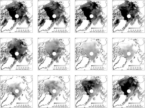
The sea spray source (PMF factor 2) also contributed in winter, when the sea surrounding Svalbard is partly frozen. Sea spray aerosols in winter and autumn may be advected from south of the ice edge or from distant open water. It has been suggested that frost flowers and the marine snow pack can be sources of sea salt (Domine et al., 2004; Kaleschke et al., 2004). Frost flowers are ice crystals which often form on the re-frozen surface of open leads and exhibit enhanced salinity of around 100 g kg⁻¹ (Perovich and Richter-Menge, 1994) and therefore could provide intense point sources of sea salt aerosol. However, in laboratory experiments with frost flowers no aerosol was observed when wind was blown across them (Roscoe et al., 2011). Thus, wind blown partly saline snow (Yang et al., 2008) appears to be a more probable source for sea-salt aerosol in the sea-ice zone. Monthly maps of the ice coverage in 2015 (Fig. 7) reveal that in winter, when the sea along the north and east coast of Svalbard is ice-covered, an area fraction of about 40% is still open water, while the sea at the west coast remains essentially ice-free during winter. Therefore, even in winter, sea-spray from open seawater likely is the most important source of sea salt aerosol at Mt. Zeppelin.

Fig. 7. Maps of average monthly open water of the Arctic Ocean, from January to December 2015. Grey colour scale: 0% open water (white), 100%: fully ice covered (black). The white circle indicates the data void near the pole that is caused by the satellite orbits.

The seasonality of marine biogenic sources, that is the MSA-based secondary source (PMF factor 6) and the marine gel sources (PMF factors 3 and 8) can be explained in terms of ocean biological activity and surface ocean stratification. Appearance of the secondary biogenic marine aerosol (PMF factor 6) in late March coincides with the Arctic spring bloom along the MIZ. The spring bloom often lasts into early June with peak abundances in April (Degerlund and Eilertsen, 2009), depending on prevailing temporal changing physical, as well as chemical and biological conditions in the surface ocean. During the spring bloom, DMS-producing diatoms are confined to the cold surface waters of the strongly stratified ocean, while the gel-producing phytoplankton species Phaeocystis pouchetii resides below the surface mixing layer (Eriksen, 2010). The main reason for P. pouchetii residing in deeper layers than diatoms is probably that the phytoplankton species can grow faster relative to diatoms when irradiance is low, taking advantage of the enhanced nutrient concentrations under the pycnocline (Eilertsen et al., 1989). The species succession during the bloom usually begins with small-celled diatoms and subsequently shifts to a mixed community of bigger diatom cells followed by a third step dominated by dinoflagellates (Margalef, 1958). Towards the end of the spring bloom, the population of diatoms and dinoflagellates declines due to zooplankton grazing and cell lysis, releasing large amounts DMS into the seawater (Leck et al., 1990). In addition, low levels of silicate and the poleward inflow of warmer North Atlantic waters (Wassmann, 2011) promote P. pouchetii at the sea surface. Less stratified and warmer waters favour the growth of P. pouchetii (Metaxatos et al., 2003; Engel et al., 2017) and the subsequent emission of extruded gels to the atmosphere by bubble bursting at the sea-air interface. Moreover, P. pouchetii have shown resistance to grazing due to their large size range and to the toxic life stage (Aanesen et al., 1998) turning them into low DMS producers. The abundance of marine gel type-1 and type-2 aerosol (PMF factors 3 and 8) in late summer and autumn is likely linked to the presence of P. pouchetii in the relatively warmer water, which limits the presence of diatoms around Svalbard compared to the conditions during late spring and summer.

The secondary biogenic marine aerosol (PMF factor 6), identified based on MSA, is an important contributor to the summertime aerosol. Chang et al. (2011) found an organic component in the marine biogenic factor that was approximately equal in mass to the amount of MSA. However, they could not firmly conclude whether the organic component was formed in secondary processes of phytoplankton-emitted biogenic VOC or emitted directly as primary organics from the ocean through a sea-spray mechanism. Observations of the aerosol composition in the Arctic summertime during pristine conditions showed secondary organic aerosol (SOA) of marine origin with low oxygen-to-carbon ratio present when MSA/nss-SO₄²⁻ was high within the boundary layer (Willis et al., 2017). Multi-year observations in the Canadian Arctic Archipelago found the increase of OM in late spring to coincide with the annual peak in MSA and low Na⁺ concentrations (Leaitch et al., 2018), suggesting that the importance of marine SOA in late spring is coupled to high biological activity in the surface ocean.

Marine gel type 1 (PMF factor 3) source peaks in autumn (mid-October) when the intensity of sunlight has ceased. Further, it contributes occasionally to PM₁ in winter. Marine gel type 1 is high in Fuc, its presence being indicative of surface-active polysaccharides. Gao et al. (2011) found high fractions of Fuc in Arctic seawater samples from open leads and from ice-covered water, that is in similar extreme conditions for marine life. Bubble scavenging of surface-active polysaccharides is a possible mechanisms leading to enrichment of polysaccharides in the SML located at the air-sea interface (Gao et al., 2012), from where it may be released to air as sea spray aerosol.

Marine gel type 2 (PMF factor 8) seems to be related to sea ice and patches of open water in the pack ice of the Fram Strait and central Arctic Ocean (Fig. 5h) because of the (partly) frozen sea during the time of occurrence (Fig. 7; October to December) of this source at Mt. Zeppelin.

The Marine gel type 2 source is high in Xyl, which is an indicator for biogenic polymers of phytoplankton origin (Hoagland et al., 1993). Xyl was also found to be abundant in Arctic seawater samples (Gao et al., 2011). Substantial Xyl was detected in an ice algal assemblage (Gao et al., 2012) loosely attached to the bottom of an ice floe collected during the ASCOS expedition when the icebreaker Oden was moored to an ice floe, which drifted passively within the pack ice. Krembs et al. (2002) have shown that Arctic sea ice diatoms release substantial quantities of extracellular polysaccharides as buffering and protection mechanism against the extreme environmental conditions, such as low temperature and high salinity.

Differences in the monosaccharide distributions of marine gel type 1 and type 2 sources might reflect the variability in biological micro algal and bacterial species and related physiology in the open water and ice-covered seawater in the pack ice, as suggested by Gao et al. (2012). In addition, from examining frost flowers grown in a freezer laboratory from a bacteria containing saline solution and frost flowers formed naturally in the central Arctic Ocean, Bowman and Deming (2010) found the concentrations of extracellular polysaccharides being elevated in the frost flowers and brine skim relative to underlying ice (up to 74 fold higher). Such elevated gel concentrations within the frost flowers may allow them to be a significant direct atmospheric source and serve as an explanation for the marine gel type 2 (PMF factor 8) attribution of Xyl. This explanation is supported by a PMF study attributing sub-micrometre OM at Barrows, Alaska, in winter to sea ice and lake ice frost flowers, based on reanalysis data of surface temperature and sea ice concentrations (Shaw et al., 2010). Overall, more research is required to link the monosaccharide distributions in airborne particles to seawater, sea ice and frost flower sources and phytoplankton species variability.

4.3 Discussion of anthropogenic sources in the inner Arctic

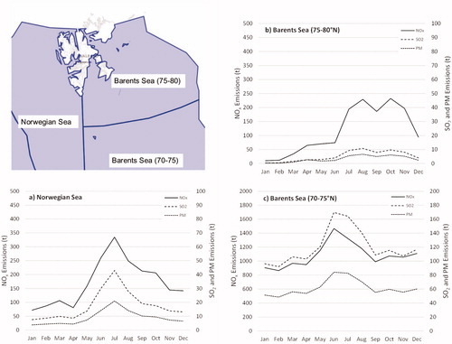
Figure 8 shows NO_X, SO₂ and PM shipping emissions at the Barents Sea and Norwegian Sea obtained from the Norwegian Coastal Administration (see Section 2.7). Monthly emissions in the Norwegian Sea and Barents Sea (70 − 75°N) in 2015 show similar patterns corresponding to shipping activity around Svalbard. Monthly emissions increase from April to June, when shipping activity reaches a maximum, followed by a decrease towards winter. Emissions at the southern part of the Barents Sea are the highest. This could be related with an extensive fishing activity in this area.

Fig. 8. Shipping emission totals of NO_X, SO₂ and PM of the ship fleet in the Norwegian Sea and Barents Sea in the months of 2015: (a) Norwegian Sea, (b) Barents Sea (75–80° N) and (c) Barents Sea (70–75° N). The geographic map in the top-left part of the figures shows the division of seas around Svalbard for shipping.

PSD analysis indicates the origin of PMF factor 7 from Siberian and inner-Arctic mixed combustion sources. The associated trajectories mainly show a long circumpolar transport route. Factor 7 is active at the end of the haze period in early summer and again in autumn. The potential source distribution does not indicate passage of air masses related to PMF factor 7 over the Barents Sea and Norwegian Sea with high shipping activity. To assess whether factor 7 is related to local pollution from ships in the Kongsfjord, passenger counts from Ny-Ålesund port were filtered according to wind direction at the Zeppelin observatory, since only winds from sector 330° to 30° will bring air from Ny-Ålesund to the mountain station. Ship traffic in Ny-Ålesund port is most intense between June and August, while during the remainder of the year only few ships were visiting the port of Ny-Ålesund. With the exception of one episode (31 July to 2 August), the mixed combustion source does not coincide with the presence of ships at Ny-Ålesund (Supporting Information Fig. S3a).

Non-crustal Vanadium (nc-V) in PM₁₀ samples collected at the Zeppelin observatory was compared to the PM₁ contribution from the mixed combustion source. After mapping the factor contribution to the sampling interval of PM₁₀, nc-V was found to coincide with the PM₁ contribution of factor 7, except from January to March and from June to August (Supporting Information Fig. S3b). Vanadium is a tracer for the long-range transport of PM-emissions from oil combustion (Isakson et al., 2001). In January to March, nc-V is connected to pollution of the Arctic haze. In the haze period, nc-V might be associated with particles in the accumulation mode (0.4–1.0 μm; Jaffrezo et al., 1993) from long-range transport (Quinn et al., 2009) in the near absence of wet removal. From June to August, nc-V was most probably from fly-ash particles emitted by ships (Zhan et al., 2014). The time series of the other metals nc-Ni, nc-Mn, nc-Cr, in PM₁₀ samples, were similar to that of nc-V. The nc-V/nc-Ni ratio during peak contributions of factor 7 was in the range 0.46 − 1.60, with an average of 0.81. The average nc-V/nc-Ni ratio from all samples was 0.63. A ratio of 0.5 is typical for combustion of coal and diesel (Pacyna and Pacyna, 2001), whereas the ratio observed for crude oil and petroleum is in the range 1 − 10 (Barwise, 1990). Thus, the nc-V/nc-Ni ratio of 0.81 for factor 7 peak contributions indicates the influence of coal and diesel combustion along the transport path of the air mass, reducing the ratio compared to the emissions from oil combustion. Based on the PSD analysis and the temporal analysis of its chemical fingerprint, it appears most likely that the mixed combustion factor is partly associated with emissions from oil extraction in Northern Russia.

4.4 Limitations of the PMF analysis

In order to provide the best fit to the observation data, the PMF user might be tempted to increase the number of factors during the analysis. Therefore, PMF has a tendency to overestimate the actual number of sources present at a given receptor site. In the present study, eight factors were required to adequately describe the PM composition at Mt. Zeppelin in 2015. This was concluded based on the physical meaning of the resolved sources, the small inter-run variability (Supporting Information Table S1), the distribution of the scaled residuals (Supporting Information Tables S2 and S3) and the rotational stability (FPEAK). The optimal number of factors has been determined by plotting Q(true)/Q_exp as function of factor number (Supporting Information Fig. S4). The small change of Q from eight to nine factors indicates that eight factors is the optimal solution. Using PMF with only seven factors resulted in a source attribution where the secondary nitrate was not separated from the secondary marine biogenic aerosol. Oxal as molecular marker, however, gives a clear indication of an aged aerosol associated with long-range atmospheric transport.

For the source apportionment in the Arctic usually a limited number of source profiles is assumed (Chang et al., 2011; Nguyen et al., 2013) due to the assumption that only few emission sources exist in the inner Arctic region. In addition, it is difficult to discern long-range transported aerosol from locally produced aerosols picked up by the air parcel on its way to the receptor site. Furthermore, an inter-comparison study of receptor models for real-world and synthetic input datasets showed that sources with well-defined chemical profiles and seasonal time trends, that make substantial contributions (>10%), can be better quantified by the PMF models whereas those with contributions to the PM mass close to 1% represent a challenge (Belis et al., 2015).

Due to its location close to the coastline Mt. Zeppelin is influenced by marine aerosols. Primary organic material is known to contribute significantly to the organic carbon (OC) in marine aerosols (Decesari et al., 2007), stemming either from marine biological, fossil fuel combustion or biomass burning sources. The sugars analysed in our study mainly represent tracer compounds for organic material from marine biological and biomass burning activities. Primary and secondary organics from fossil fuel sources have not been taken into account directly or indirectly because measurements of OC were not available. This may have caused an underestimation of the mixed combustion source to total PM₁ in the PMF analysis. Zhan et al. (2014) reported summertime OC concentrations measured in the settlement of Ny-Ålesund in the range 13.8–64.4 ng m⁻³, with a mean of 32.8 ng m⁻³. High OC concentrations were found in samples influenced by emissions from cruise ships visiting the port of Ny-Ålesund.

One prerequisite for using receptor modelling is that the chosen marker compounds do not react chemically or undergo phase transition, for example, by re-volatilisation on their path from source to receptor site. However, using semi-volatile organic compounds may still work well during meteorological conditions, which preserve the original compound to a high extent (Belis et al., 2013). In the case of oxalic acid (measured in the form of oxalate), which is used as marker for aged aerosol, associated with long-range atmospheric transport, in our study this should be sufficiently fulfilled. Due to its low volatility, Oxal will be predominantly associated to the particulate phase. During the transport into a colder region, it is unlikely that Oxal evaporates from the particles. Laboratory photolysis experiments showed that Oxal can be oxidised by the OH–radical in the aqueous phase but that it is relatively stable in the absence of iron (Fe²⁺, Fe³⁺) (Pavuluri and Kawamura, 2012). The atmospheric lifetime of Oxal thus depends on the intensity of sunlight and the presence of iron in the aerosol. It is therefore not possible to firmly establish the possible degradation of Oxal during the transport path.

5. Conclusions

The study identified the sources of sub-micrometre aerosol at Mt. Zeppelin observatory in 2015 using PMF and potential source distributions based on back trajectories. Main constituents of the chemically reconstructed PM₁ were organic matter followed by ammonium sulphate and sea salt. Black carbon was mainly associated with the biomass-burning factor. The winter average of measured BC was about three times higher than the summer average. In winter, residential wood combustion and fossil fuel combustion from Fenno-Scandinavia and from inner-Arctic sources presumably contributed to the biomass-burning factor whereas during summer, plumes from wildfires originating in Arctic Canada and Alaska dominated the biomass-burning factor. The mixed combustion factor contributed mainly in spring and autumn. The most likely origin of this anthropogenic source is oil and gas extraction activities in Northern Siberia. No direct evidence for the contribution of inner-Arctic ship traffic was found, but the identified sea spray factor showed mixing with combustion particles that presumably were from shipping emissions.

PMF analysis is advantageous because it does not require a priori knowledge about the chemical profile of aerosol sources. This is in particular useful for source apportionment in the Arctic region because:

1. The seasonality and strength of the biogenic inner Arctic aerosol sources are not well characterized, and

2. The modelling of long-range transport of aerosols into the Arctic using atmospheric chemistry transport models is limited by the reliability of emission inventories and the accuracy of hemispheric transport patterns.

The PSD analysis proved to be a useful method for the identification of potential source regions of PMF factors, especially in the Arctic where no dense network of meteorological and aerosol measurement stations exists.

The presented PMF analysis identified three sources with minor contribution on an annual basis, the two marine gel sources and the mixed combustion sources, but they were found to be significant in the uncertainty analysis. The use of monosaccharides as molecular markers and the extremely low detection limits (MDL of the analytical method in the order of 10⁻⁵ng m⁻³) for these markers, enabled accurate attribution to the two marine gel factors in the PMF analysis, even at the low measured concentrations of particulate sugars in ambient PM₁ samples. Levoglucosan, which is frequently used as marker for biomass burning, was unfortunately not included in the chemical analysis. In the present study, nss-K⁺ was used as a marker for emissions from biomass burning since it is known to be a good tracer of biomass burning aerosols (Niemi et al., 2004).

Ice-covered sea areas in the Arctic Ocean during summer have nearly halved since the 1980s. With the continued retreat and thinning of sea ice, the Arctic region is becoming more accessible for human activity, most importantly for transit shipping and fossil fuel extraction. The influence of increasing oil and gas extraction activities in the inner-Arctic and northern Russia (Stohl et al., 2013) on the sub-micrometre aerosol composition in the Arctic background air needs thorough attention in the coming years. Observations at the receptor sites in conjunction with receptor modelling might help to assess the relevance of the previously unaccounted gas flaring emissions of BC resulting from new Arctic extraction activities.

In late spring and summer, secondary marine biogenic aerosol from the photo-oxidation of DMS emitted from the surrounding seas constitutes an important contribution to the sub-micrometre particulate matter. DMS oxidation products play a prominent role in the formation of new particles in the summertime Arctic. Based on a 11-year record of aerosol size distributions at the Mt. Zeppelin observatory, Dall Osto et al. (2017) found that highest daily average concentrations of MSA were associated with nucleation event days in summer. The occurrence of new particle events was anti-correlated with sea ice extent over a decade, suggesting that the frequency of nucleation events will increase as more open water areas with high biological productivity emerge after sea ice retreat (Dall Osto et al., 2017).

Previous observations of marine gels in the high Arctic north of 80°N (Leck and Bigg, 2005b; Leck et al, 2013) on-board the ice-breaker Oden have been limited to summer. Particle number concentrations of marine gels, observed in clean air over the Arctic, have been found to increase from June through August, related to ocean biological activity (Heintzenberg et al., 2017). The new finding of marine gel sources in autumn and winter broadens our picture of their abundance and seasonality. The small contribution of the marine gel sources at Mt. Zeppelin observatory in summer as opposed to regions closer to the North Pole is attributed to differences in ocean biology, the vertical distribution of phytoplankton, and the earlier start of the summer season. Obviously, the related mechanisms by which the marine gels become airborne are different during the freezing of sea ice in autumn and winter from those that are acting at the sea-air interface during the spring bloom and the ice melt in summer.

In autumn, ice formation during the freeze-up period extrudes salt brine and dissolved organic matter, including marine polymer gels. Wind erosion of frost flowers high in extracellular polysaccharides may offer a direct dispersal mechanism (Bowman and Deming, 2010) by which marine gel particles become airborne. Frost flower erosion and sea-ice brine extrusions to water and air during freeze-up are mechanisms by which fluxes of marine biological particles to the atmosphere might be coupled with extensive first-year sea-ice formation in autumn and winter (Gabric et al., 2018).

Primary marine polymer gels were found to undergo fragmentation in air (Leck and Bigg, 2010; Karl et al., 2013; Heintzenberg et al., 2015), turning them into a potentially important source of cloud condensation nuclei (CCN) in the pristine air of the high Arctic north of 80°N during the summer season (Orellana et al., 2011). It remains an open question how the abundance of marine polymer gels, which, due to their surface-active properties, have a high potential for cloud droplet activation (Ovadnevaite et al., 2011; Leck and Svensson, 2015) affect the melting and freezing of the perennial sea ice. Matrai and Leck (2012) suggested that low-level clouds forming during the peak-melt season at the end of summer could cool the surface, thereby influencing the timing of the autumn freeze-up and the thickness of the winter ice. However, the potentially cooling processes might be counteracted by increasingly open water areas in summer associated with higher sea-air fluxes of primary biological aerosol and DMS. Enhanced formation of secondary biogenic particles through condensation of DMS oxidation products together with emissions of black carbon and condensable precursors from transit shipping and gas flaring might result in higher numbers of CCN, affecting the abundance of low-level clouds and fog in summer.

Acknowledgements

The U.S. NOAA-ARL kindly provided the HYSPLIT trajectory algorithm and the necessary global meteorological data for utilising HYSPLIT. NSIDC kindly provided the ice maps of the present study. Norwegian Coastal Administration (Kystverket) is thanked for making available the monthly ship emission data on their internet platform. Measurement data of the EMEP monitoring program at the Zeppelin observatory were extracted from the EBAS database, which is maintained and further developed by NILU.

Disclosure statement

No potential conflict of interest was reported by the authors.

Additional information

Funding

The Svalbard Environmental Protection Fund (Svalbard Miljøvernfond) is acknowledged for financial support of the project SHIMATE ‘Ship Traffic Particulate Matter Emissions’, which in part provided the data basis for the present study.

References

- Aanesen, R. T., Eilertsen, H. C. and Stabell, O. B. 1998. Light-induced toxic properties of the marine alga Phaeocystis pouchetii towards cod larvae. Aquat. Toxicol. 40, 109–121. doi:10.1016/S0166-445X(97)00056-8
- Aas, W., Fiebig, M., Platt, S., Solberg, S. and Yttri, K. E. 2016. Monitoring of Long-Range Transported Air Pollutants in Norway. Annual Report 2015, Miljødirektoratet rapport, M-652/2016, NILU OR, 13/2016, Norsk Institutt for Luftforskning, Kjeller, Norway.
- ACIA 2014. Impacts of a Warming Arctic: Arctic Climate Impact Assessment, ACIA Overview report, Cambridge University Press, Cambridge, UK, p. 140.
- Barwise, A. J. G. 1990. Role of nickel and vanadium in petroleum classification. Energy Fuels 4, 647–652. doi:10.1021/ef00024a005
- Belis, C. A., Karagulian, F., Larsen, B. B. and Hopke, P. K. 2013. Critical review and meta-analysis of ambient particulate matter source apportionment using receptor models in Europe. Atmos. Environ. 69, 94–108. doi:10.1016/j.atmosenv.2012.11.009
- Belis, C. A., Pernigotti, D., Karagulian, F., Pirovano, G., Larsen, B. R. and co-authors. 2015. A new methodology to assess the performance and uncertainty of source apportionment models II: the results of two European intercomparison exercises. Atmos. Environ. 119, 35–44. doi:10.1016/j.atmosenv.2015.08.002
- Benner, R., Pakulski, J. D., McCarthy, M. Hedges, J. I., and Hatcher, P. 1992. Bulk chemical characteristics of dissolved organic matter in the ocean. Science 255, 1561–1564.
- Berg, T., Aas, W., Pacyna, J., Uggerud, H. T. and Vadset, M. 2008. Atmospheric trace metal concentrations at Norwegian background sites during 25 years and its relation to European emissions. Atmos. Environ. 42, 7494–7501. doi:10.1016/j.atmosenv.2008.05.020
- Bigg, E. K. and Leck, C. 2001. Properties of the aerosol over the central Arctic Ocean. J. Geophys. Res. 106, 32101–32109. doi:10.1029/1999JD901136
- Bigg, E. K. and Leck, C. 2008. The composition of fragments of bubbles bursting at the ocean surface. J. Geophys. Res 113, D11209. doi:10.1029/2007JD009078
- Bowman, J. S. and Deming, J. W. 2010. Elevated bacterial abundance and exopolymers in saline frost flowers with implications for atmospheric chemistry and microbial dispersal. Geophys. Res. Lett. 37, L13501.
- Brimblecombe, P. and Clegg, S. 1988. The solubility and behavior of acidic gases in the marine aerosol. J. Atmos. Chem. 7, 1–18. doi:10.1007/BF00048251
- Brown, S. G., Eberly, S., Paatero, P. and Norris, G. A. 2015. Methods for estimating uncertainty in PMF solutions: Examples with ambient air and water quality data and guidance on reporting PMF results. Sci. Total Environ. 518–519, 626–635. doi:10.1016/j.scitotenv.2015.01.022
- Browse, J., Carslaw, K. S., Arnold, S. R., Pringle, K. and Boucher, O. 2012. The scavenging process controlling the seasonal cycle in Arctic sulphate and black carbon aerosol. Atmos. Chem. Phys. 12, 6775–6798. doi:10.5194/acp-12-6775-2012
- Cachier, H., Liousse, C., Buat‐Menard, P. and Gaudichet, A. 1995. Particulate content of savanna fire emissions. J. Atmos. Chem. 22, 123–148. doi:10.1007/BF00708185
- Carpenter, L. J., Archer, S. D. and Beale, R. 2012. Ocean-atmosphere trace gas exchange. Chem. Soc. Rev. 41, 6473–6506. doi:10.1039/c2cs35121h
- Carslaw, K. S., Lee, L. A., Reddington, C. L., Pringle, K. J., Rap, A. and co-authors. 2013. Large contribution of natural aerosols to uncertainty in indirect forcing. Nature 503, 67–71. doi:10.1038/nature12674
- Chang, R. Y.-W., Leck, C., Graus, M., Müller, M., Paatero, J. and co-authors. 2011. Aerosol composition and sources in the central Arctic Ocean during ASCOS. Atmos. Chem. Phys. 11, 10619–10636. doi:10.5194/acp-11-10619-2011
- Chin, W.-C., Orellana, M. V. and Verdugo, P. 1998. Spontaneous assembly of marine dissolved organic matter into polymer gels. Nature 391, 568–572. doi:10.1038/35345
- Dall Osto, M., Beddows, D. C. S., Tunved, P., Krejci, R., Ström, J. and co-authors. 2017. Arctic sea ice melt leads to atmospheric new particle formation. Sci. Rep. 7, 3318 doi:10.1038/s41598-017-03328-1
- Dalsøren, S. B., Samset, B. H., Myhre, G., Corbett, J. J., Minjares, R. and co-authors. 2013. Environmental impacts of shipping in 2030 with a particular focus on the Arctic region. Atmos. Chem. Phys. 13, 1941–1955. doi:10.5194/acp-13-1941-2013
- Das, R., Granat, L., Leck, C., Praveen, P. S. and Rodhe, H. 2011. Chemical composition of rainwater at Maldives Climate Observatory at Hanimaadhoo (MCOH). Atmos. Chem. Phys. 11, 3743–3755. doi:10.5194/acp-11-3743-2011
- Decho, A. W. 1990. Microbial exopolymer secretions in ocean environments: their role(s) in food webs and marine processes. Oceanogr. Mar. Biol. 28, 73–153.
- Decesari, S., Mircea, M., Cavalli, F., Fuzzi, S., Moretti, F. and co-authors. 2007. Source attribution of water-soluble organic aerosol by nuclear magnetic resonance spectroscopy. Environ. Sci. Technol. 41, 2479–2484. doi:10.1021/es061711l
- Degerlund, M. and Eilertsen, H. C. 2009. Main species characteristics of phytoplankton spring blooms in NE Atlantic and Arctic waters (68–80° N). Est. Coasts 33, 242–269. doi:10.1007/s12237-009-9167-7
- Domine, F., Sparapani, R., Ianniello, A. and Beine, H. J. 2004. The origin of sea salt in snow on Arctic sea ice and in coastal regions. Atmos. Chem. Phys. 4, 2259–2271. doi:10.5194/acp-4-2259-2004
- Draxler, R. R. and Rolph, G. D. 2003. HYSPLIT (Hybrid Single-Particle Lagrangian Integrated Trajectory) Model access via NOAA ARL READY. NOAA Air Resources Lab., Silver Spring, MD. Online at: http://ready.arl.noaa.gov/HYSPLIT.php,
- Eckhardt, S., Hermansen, O., Grythe, H., Fiebig, M., Stebel, K. and co-authors. 2013. The influence of cruise ship emissions on air pollution in Svalbard – a harbinger of a more polluted Arctic? Atmos. Chem. Phys. 13, 8401–8409. doi:10.5194/acp-13-8401-2013
- Eilertsen, H. C., Taasen, J. P. and WesIawski, J. M. 1989. Phytoplankton studies in the fjords of West Spitzbergen: physical environment and production in spring and summer. J. Plankton Res. 11, 1245–1260. doi:10.1093/plankt/11.6.1245
- Eleftheriadis, K., Vratolis, S. and Nyeki, S. 2009. Aerosol black carbon in the European Arctic: measurements at Zeppelin station, Ny-Ålesund, Svalbard from 1998-2007. Geophys. Res. Lett. 36, L02809. DOI:10.1029/2008GL035741.
- EMEP 2014. (). Manual for Sampling and Chemical Analysis. EMEP/CCC Report 1/95. Norwegian Institute for Air Research, Kjeller, Norway.. Online at: https://www.nilu.no/projects/ccc/manual/download/cccr1-95rev.pdf.
- Engel, A., Piontek, J., Metfies, K., Endres, S., Sprong, P. and co-authors. 2017. Inter-annual variability of transparent exopolymer particles in the Arctic Ocean reveals high sensitivity to ecosystem changes. Sci. Rep. 7, 4129. doi:10.1038/s41598-017-04106-9
- Engling, G., Carrico, C. M., Kreidenweis, S. M., Collett, J. L., Jr., Day, D. E. and co-authors. 2006. Determination of levoglucosan in biomass combustion aerosol by high-performance anion-exchange chromatography with pulsed amperometric detection. Atmos. Environ. 40, 299–S311. doi:10.1016/j.atmosenv.2005.12.069
- Engström, J. E. and Leck, C. 2011. Reducing uncertainties associated with filter-based optical measurements of light absorbing carbon particles with chemical information. Atmos. Meas. Tech. 4, 1553–1566. doi:10.5194/amt-4-1553-2011
- Engström, J. E. and Leck, C. 2017. Seasonal variability in atmospheric black carbon at three stations in South-Asia. Tellus B 69, 1331102. doi:10.1080/16000889.2017.1331102
- Eriksen, G. K. 2010. Aspects of phytoplankton spring blooms in northern coastal/shelf areas: Diatoms vs. Phaeocystis pouchetii (Hariot, Lagerheim). BIO-3950 Master’s thesis in Biology, University of Tromsø, November 2010.
- Frossard, A. A., Russell, L. M., Burrows, S. M., Elliott, S. M., Bates, T. S. and co-authors. 2014. Sources and composition of submicron organic mass in marine aerosol particles. J. Geophys. Res. Atmos. 119, 12977–13003. doi:10.1002/2014JD021913
- Frossard, A. A., Shaw, P., Russell, L. M., Kroll, J. H., Canagaratna, M. J. and co-authors. 2011. Springtime Arctic haze contributions of submicron organic particles from European and Asian combustion sources. J. Geophys. Res. 116, D05205.
- Fu, P. Q., Kawamura, K., Chen, J., Charrière, B. and Sempéré, R. 2013. Organic molecular composition of marine aerosols over the Arctic Ocean in summer: contributions of primary emission and secondary aerosol formation. Biogeosciences 10, 653–667. doi:10.5194/bg-10-653-2013
- Gabric, A., Matrai, P., Jones, G. and Middleton, J. 2018. The nexus between sea ice and polar emissions of marine biogenic aerosols. Bull. Amer. Meteor. Soc. 99, 61–68. doi:10.1175/BAMS-D-16-0254.1
- Gao, Q., Leck, C., Rauschenberg, C. and Matrai, P. A. 2012. On the chemical dynamics of extracellular polysaccharides in the high Arctic surface microlayer. Ocean Sci. 8, 401–418. doi:10.5194/os-8-401-2012
- Gao, Q., Nilsson, U., Ilag, L. L. and Leck, C. 2011. Monosaccharide compositional analysis of marine polysaccharides by hydrophilic interaction liquid chromatography-tandem mass spectrometry. Anal. Bioanal. Chem. 399, 2517–2529. doi:10.1007/s00216-010-4638-z
- Hagen, D., Vistad, O. I., Eide, N. E., Flyen, A. C. and Fangel, K. 2012. Managing visitor sites in Svalbard: from a precautionary approach towards knowledge-based management. Polar Res. 31, 18432. doi:10.3402/polar.v31i0.18432
- Hansen, J. and Nazarenko, L. 2004. Soot climate forcing via snow and ice albedos. Proc. Natl. Acad. Sci. USA 101, 423–428. doi:10.1073/pnas.2237157100
- Hamacher-Barth, E., Leck, C. and Jansson, K. 2016. Size resolved morphological properties of the high Arctic summer aerosol during ASCOS-2008. Atmos. Chem. Phys. 16, 1–17.
- Heidam, N. Z. 1981. Review: Aerosol fractionation by sequential filtration with nuclepore filters. Atmos. Environ. (1967) 15, 1981, 891–904. doi:10.1016/0004-6981(81)90088-3
- Heintzenberg, J. 1982. Size-segregated measurements of particulate elemental carbon and aerosol light absorption at remote Arctic locations. Atmos. Environ. 16, 2461–2469. doi:10.1016/0004-6981(82)90136-6
- Heintzenberg, J. 1988. A processor-controlled multisample soot photometer. Aerosol Sci. Technol. 8, 227–233. doi:10.1080/02786828808959185
- Heintzenberg, J. 1989. Arctic haze: air pollution in polar regions. Ambio 18, 50–55.
- Heintzenberg, J. and Leck, C. 1994. Seasonal variation of the atmospheric aerosol near the top of the marine boundary layer over Spitsbergen related to the Arctic Sulphur cycle. Tellus 46B, 52–67.
- Heintzenberg, J., Hermann, M., Weigelt, A., Clarke, A., Kapustin, V. and co-authors. 2011. Near-global aerosol mapping in the upper troposphere and lowermost stratosphere with data from the CARIBIC project. Tellus B 63, 875–890. doi:10.1111/j.1600-0889.2011.00578.x
- Heintzenberg, J., Birmili, W., Seifert, P., Panov, A., Chi, X. and co-authors. 2013. Mapping the aerosol over Eurasia from the Zotino Tall Tower (ZOTTO). Tellus B 65, 20062, 1–13.
- Heintzenberg, J., Leck, C. and Tunved, P. 2015. Potential source regions and processes of aerosol in the summer Arctic. Atmos. Chem. Phys. 15, 6487–6502. doi:10.5194/acp-15-6487-2015
- Heintzenberg, J., Tunved, P., Galí, M. and Leck, C. 2017. New particle formation in the Svalbard 2006-2015. Atmos. Chem. Phys. 17, 6153–6175. doi:10.5194/acp-17-6153-2017
- Hillamo, R. E., Kerminen, V.-M., Maenhaut, W., Jaffrezo, J.-L., Balachandran, S. and co-authors. 1993. Size distributions of atmospheric trace elements at dye 3, Greenland – I. Distribution characteristics and dry deposition velocities. Atmos. Environ. A 27, 2787–2802. doi:10.1016/0960-1686(93)90311-L
- Hoagland, K. D., Rosowski, J. R., Gretz, M. R. and Roemer, S. C. 1993. Diatom extracellular polymeric substances: function, fine structure, chemistry, and physiology. J. Phycol. 29, 537–566. doi:10.1111/j.0022-3646.1993.00537.x
- Hole, L. R., and Christensen, J., Ginzburg, V. A., Makarov, V., Polishok, A. I., Ruoho-Airola, T., and Vasilenko, V. N. 2006. Concentrations and Deposition of Acidifying Air Pollutants. In: Arctic Pollution 2006. Arctic Monitoring and Assessment Programme (AMAP), Oslo, Norway, p. 35.
- Hwang, I. J. and Hopke, P. K. 2006. Comparison of source apportionments of fine particulate matter at two San Jose STN sites. J. Air Waste Manage. Assoc. 56, 1287–1300. doi:10.1080/10473289.2006.10464586
- Isakson, J., Persson, T. A. and Lindgren, E. S. 2001. Identification and assessment of ship emissions and their effects in the harbour of Göteborg, Sweden. Atmos. Environ. 35, 3659–3666. doi:10.1016/S1352-2310(00)00528-8
- Jaffrezo, J.-L., Hillamo, R. E., Davidson, C. I. and Maenhaut, W. 1993. Size distributions of atmospheric trace elements at dye 3, Greenland – II. Sources and transport. Atmos. Environ. A 27, 2803–2814. https://doi.org/10.1016/0960-1686(93)90312-M. doi:10.1016/0960-1686(93)90312-M
- Jeffries, M. O. and Richter-Menge, J. 2015. The Arctic, in: “State of the Climate in 2014. Bull. Amer. Meteor. Soc. 96, S127–S148.
- John, W., Hering, S., Reischl, G., Sasaki, G. and Goren, S. 1983. Characteristics of Nuclepore filters with large pore size – II. Filtration properties. Atmos. Environ. (1967) 17, 373–382. doi:10.1016/0004-6981(83)90054-9
- Kaleschke, L., Richter, A., Burrows, J., Afe, O., Heygster, G. and co-authors. 2004. Frost flowers on sea ice as a source of sea salt and their influence on tropospheric halogen chemistry. Geophys. Res. Lett. 31, L16114. doi:10.1029/2004GL020655
- Karl, M., Gross, A., Leck, C. and Pirjola, L. 2007. Intercomparison of dimethylsulfide oxidation mechanisms for the marine boundary layer: gaseous and particulate sulfur constituents. J. Geophys. Res. 112, D15304. 914. doi:10.1029/2006JD007914
- Karl, M., Leck, C., Coz, E. and Heintzenberg, J. 2013. Marine nanogels as a source of atmospheric nanoparticles in the high Arctic. Geophys. Res. Lett. 40, 3738–3743. doi:10.1002/grl.50661
- Krembs, C., Eicken, H., Junge, K. and Deming, J. W. 2002. High concentrations of exopolymeric substances in Arctic winter sea ice: implications for the polar ocean carbon cycle and cryoprotection of diatoms. Deep-Sea Res. 49, 2163–2181. doi:10.1016/S0967-0637(02)00122-X
- Law, K. S. and Stohl, A. 2007. Arctic air pollution: origins and impacts. Science 315, 1537–1540. doi:10.1126/science.1137695
- Leaitch, W. R., Russell, L. M., Liu, J., Kolonjari, F., Toom, D. and co-authors. 2018. Organic functional groups in the submicron aerosol at 82.5° N, 62.5° W from 2012 to 2014. Atmos. Chem. Phys. 18, 3269–3287. doi:10.5194/acp-18-3269-2018
- Leck, C. and Bigg, E. K. 2005a. Source and evolution of the marine aerosol – a new perspective. Geophys. Res. Lett. 32, L19803. DOI:10.1029/2005GL023651.
- Leck, C. and Bigg, E. K. 2005b. Biogenic particles in the surface microlayer and overlaying atmosphere in the central Arctic Ocean during summer. Tellus B 57, 305–316. doi:10.1111/j.1600-0889.2005.00148.x
- Leck, C. and Bigg, E. K. 2010. New particle formation of marine biological origin. Aerosol Sci. Technol. 44, 570–577. doi:10.1080/02786826.2010.481222
- Leck, C. and Persson, C. 1996. The central Arctic Ocean as a source of dimethyl sulfide: seasonal variability in relation to biological activity. Tellus B 48, 156–177. doi:10.3402/tellusb.v48i2.15834
- Leck, C. and Persson, C. 1996b. Seasonal and short-term variability in dimethyl sulfide, sulfur dioxide and biogenic sulfur and sea salt aerosol particles in the arctic marine boundary layer during summer and autumn. Tellus B 48, 272–299. doi:10.3402/tellusb.v48i2.15891
- Leck, C. and Svensson, E. 2015. Importance of aerosol composition and mixing state for cloud droplet activation over the Arctic pack ice in summer. Atmos. Chem. Phys. 15, 2545–2568. doi:10.5194/acp-15-2545-2015
- Leck, C., Gao, Q., Mashayekhy Rad, F. and Nilsson, U. 2013. Size-resolved atmospheric particulate polysaccharides in the high summer Arctic. Atmos. Chem. Phys. 13, 12573–12588. doi:10.5194/acp-13-12573-2013
- Leck, C., Larsson, U., Bågander, L. E., Johansson, S. and Hajdu, S. 1990. Dimethyl sulfide in the Baltic Sea: annual variability in relation to biological activity. J. Geophys. Res. 95, 3353–3363. doi:10.1029/JC095iC03p03353
- Leck, C., Norman, M., Bigg, E. K. and Hillamo, R. 2002. Chemical composition and sources of the high Arctic aerosol relevant for cloud formation. J. Geophys. Res. 107, 4135. doi:10.1029/2001JD001463
- Lim, H.-J., Carlton, A. and Turpin, B. J. 2005. Isoprene forms secondary organic aerosol through cloud processing: Model simulations. Environ. Sci. Technol. 39, 4441–4446. doi:10.1021/es048039h
- López-Aparicio, S., Karl, M., Leck, C. and Bäcklund, A. 2016. SHIPMATE – ship traffic particulate matter emissions. NILU report 1/2016, ISBN: 978-82-425-2814-8, Norwegian Institute for Air Research, Kjeller, Norway, p. 29.
- Lundén, J., Svensson, G., Wisthaler, A., Tjernström, M., Hansel, A. and co-authors. 2010. The vertical distribution of atmospheric DMS in the high Arctic summer. Tellus B 62, 160–171. doi:10.1111/j.1600-0889.2010.00458.x
- Malm, W. C., Pitchford, M. L., McDade, C. and Ashbaugh, L. L. 2007. Coarse particle speciation at selected locations in the rural continental United States. Atmos. Environ. 41, 2225–2239. doi:10.1016/j.atmosenv.2006.10.077
- Margalef, R. 1958. Temporal Succession and Spatial Heterogeneity in Phytoplankton. Perspectives in Marine Biology. Berkeley, CA, USA: University of California Press, p. 323–348.
- Matrai, P. and Leck, C. 2012. A silver lining to Arctic clouds? Global Change 79, 8–11.
- Mårtensson, E. M., Nilsson, E. D., Leeuw, G. D., Cohen, L. H. and Hansson, H.-C. 2003. Laboratory simulations and parameterization of the primary marine aerosol production. J. Geophys. Res. 108, 4297.
- Metaxatos, A., Panagiotopoulos, C. and Ignatiades, L. 2003. Monosaccharide and aminoacid composition of mucilage material produced from a mixture of four phytoplanktonic taxa. J. Exp. Mar. Biol. Ecol. 294, 203–217. doi:10.1016/S0022-0981(03)00269-7
- Mochida, M., Umemoto, N., Kawamura, K. and Uematsu, M. 2003. Bimodal size distribution of C2–C4 dicarboxylic acids in the marine aerosols. Geophys. Res. Lett. 30, 1672.
- Monahan, E. C. and O'Muircheartaigh, I. G. 1986. Review article: whitecaps and the passive remote sensing of the ocean surface. Int. J. Remote Sens. 7, 627–642. doi:10.1080/01431168608954716
- Ng, N. L., Canagaratna, M. R., Zhang, Q., Jimenez, J. L., Tian, J. and co-authors. 2010. Organic aerosol components observed in Northern Hemispheric datasets from Aerosol Mass Spectrometry. Atmos. Chem. Phys. 10, 4625–4641. doi:10.5194/acp-10-4625-2010
- Nguyen, Q. T., Skov, H., Sørensen, L. L., Jensen, B. J., Grube, A. G. and co-authors. 2013. Source apportionment of particles at Station Nord, North East Greenland during 2008–2010 using COPREM and PMF analysis. Atmos. Chem. Phys. 13, 35–49. doi:10.5194/acp-13-35-2013
- Niemi, J. V., Tervahattu, H., Vehkamäki, H., Kulmala, M., Koskentalo, T. and co-authors. 2004. Characterization and source identification of a fine particle episode in Finland. Atmos. Environ. 38, 5003–5012. doi:10.1016/j.atmosenv.2004.06.023
- Nilsson, E. D., Rannik, Ü., Swietlicki, E., Leck, C., Aalto, A. A. and co-authors. 2001. Turbulent aerosol fluxes over the Arctic Ocean 2.Wind-driven sources from the sea. J. Geophys. Res. 106, 32139–32154. doi:10.1029/2000JD900747
- Nolte, C. G., Schauer, J. J., Cass, G. R. and Simoneit, B. R. T. 2001. Highly polar organic compounds present in wood smoke and in the ambient atmosphere. Environ. Sci. Technol. 35, 1912–1919. doi:10.1021/es001420r
- Norris, G., Duvall, R., Brown, S. and Bai, S. 2014. EPA Positive Matrix Factorization (PMF) 5.0, Fundamentals and User Guide. EPA/600/R-14/108 (NTIS PB2015-105147). U.S. Environmental Protection Agency, Washington, DC.
- Norris, S. J., Brooks, I. M., de Leeuw, G., Sirevaag, A., Leck, C. and co-authors. 2011. Measurements of bubble size spectra within leads in the Arctic summer pack ice. Ocean Sci. 7, 129–139. doi:10.5194/os-7-129-2011
- Northwestern University 2015. Alaska’s 2015 Fire Season Consumes 5.1 Million Acres of Forest. Online at: http://climatechange.medill.northwestern.edu/2015/12/02/fires-in-alaska/.
- Orellana, M. V., Matrai, P. A., Leck, C., Rauschenberg, C. D., Lee, A. M. and co-authors. 2011. Marine microgels as a source of cloud condensation nuclei in the high arctic. Proc. Natl. Acad. Sci. USA. 108, 13612–13617. doi:10.1073/pnas.1102457108
- Ovadnevaite, J., Ceburnis, D., Martucci, G., Bialek, J., Monahan, C. and co-authors. 2011. Primary marine organic aerosol: a dichotomy of low hygroscopicity and high CCN activity. Geophys. Res. Lett. 38, L21806.
- Ødemark, K., Dalsøren, S. B., Samset, B. H., Berntsen, T. K., Fuglestvedt, J. S. and co-authors. 2012. Short-lived climate forcers from current shipping and petroleum activities in the Arctic. Atmos. Chem. Phys. 12, 1979–1993. doi:10.5194/acp-12-1979-2012
- Paatero, P. 1997. Least square formulation of robust non-negative factor analysis. Chemometr. Intell. Lab. Syst. 37, 23–35. doi:10.1016/S0169-7439(96)00044-5
- Paatero, P. and Hopke, P. K. 2003. Discarding or downweighting high-noise variables in factor analytic models. Anal. Chim. Acta 490, 277–289. doi:10.1016/S0003-2670(02)01643-4
- Paatero, P., Hopke, P. K., Song, X. H. and Ramadan, Z. 2002. Understanding and controlling rotations in factor analytic models. Chemometr. Intell. Lab. Syst. 60, 253–264. doi:10.1016/S0169-7439(01)00200-3
- Pacyna, J. M. and Pacyna, E. G. 2001. An assessment of global and regional emissions of trace metals to the atmosphere from anthropogenic sources worldwide. Dossiers. Environ. 9, 269–298. doi:10.1139/a01-012
- Pachon, J. E., Weber, R. J., Zhang, X., Mulholland, J. A. and Russell, A. G. 2013. Revising the use of potassium (K) in the source apportionment of PM2.5. Atmos. Pollut. Res. 4, 14–21. doi:10.5094/APR.2013.002
- Park, K.-T., Lee, K., Yoon, Y.-Y., Lee, H.-W., Kim, H.-C. and co-authors. 2013. Linking atmospheric dimethyl sulfide and the Arctic Ocean spring bloom. Geophys. Res. Lett. 40, 155–160. doi:10.1029/2012GL054560
- Pavuluri, C. M. and Kawamura, K. 2012. Evidence for 13-carbon enrichment in oxalic acid via iron catalyzed photolysis in aqueous phase. Geophys. Res. Lett. 39, L03802.
- Perovich, D. K. and Richter-Menge, J. A. 1994. Surface characteristics of lead ice. J. Geophys. Res. 99, 16,341–16,350. doi:10.1029/94JC01194
- Pio, C. A., Legrand, M., Alves, C. A., Oliveira, T., Afonso, J. and co-authors. 2008. Chemical composition of atmospheric aerosols during the 2003 summer intense forest fire period. Atmos. Environ. 42, 7530–7543. doi:10.1016/j.atmosenv.2008.05.032
- Polissar, A. V., Hopke, P. K., Paatero, P., Malm, W. C. and Sisler, J. F. 1998. Atmospheric aerosol over Alaska 2. Elemental composition and sources. J. Geophys. Res. 103, 19045–19057. doi:10.1029/98JD01212
- Quinn, P. K., Bates, T. S., Schulz, K. and Shaw, G. E. 2009. Decadal trends in aerosol chemical composition at Barrow, Alaska: 1976–2008. Atmos. Chem. Phys. 9, 8883–8888. doi:10.5194/acp-9-8883-2009
- Quinn, P. K., Shaw, G., Andrews, E., Dutton, E. G., Ruoho-Airola, T. and co-authors. 2007. Arctic haze: current trends and knowledge gaps. Tellus B 59, 99–114. doi:10.1111/j.1600-0889.2006.00236.x
- Rahn, K. A. and McCaffrey, R. J. 1980. On the origin and transport of the winter Arctic aerosol. Ann. NY. Acad. Sci. 338, 486–503. doi:10.1111/j.1749-6632.1980.tb17142.x
- Roiger, A., Thomas, J.-L., Schlager, H., Law, K. S., Kim, J. and co-authors. 2015. Quantifying emerging local anthropogenic emissions in the Arctic region: the ACCESS aircraft campaign experiment. Bull. Amer. Meteor. Soc. 96, 441–460. doi:10.1175/BAMS-D-13-00169.1
- Roscoe, H. K., Brooks, B., Jackson, A. V., Smith, M. H., Walker, S. J. and co-authors. 2011. Frost flowers in the laboratory: Growth, characteristics, aerosol, and the underlying sea ice. J. Geophys. Res. 116, D12301. doi:10.1029/2010JD015144
- Russell, L. M., Hawkins, L. N., Frossard, A. A., Quinn, P. K. and Bates, T. S. 2010. Carbohydrate-like composition of submicron atmospheric particles and their production from ocean bubble bursting. Proc. Natl. Acad. Sci. USA 107, 6652–6657. doi:10.1073/pnas.0908905107
- Salter, M. E., Hamacher-Barth, E., Leck, C., Werner, J., Johnson, C. M. and co-authors. 2016. Calcium enrichment in sea spray aerosol particles. Geophys. Res. Lett. 43, 8277–8285.
- Seinfeld, J. H. and Pandis, S. N. 2006. Atmospheric Chemistry and Physics: From Air Pollution to Climate Change. 2nd ed. Wiley-Interscience, Hoboken, NJ. ISBN: 0471720186, 20 9780471720188
- Serreze, M. C. and Barry, R. G. 2011. Processes and impacts of Arctic amplification: a research synthesis. Global Planetary Change 77, 85–96. doi:10.1016/j.gloplacha.2011.03.004
- Sharma, S., Andrews, E., Barrie, L., Ogren, J. and Lavou, D. 2006. Variations and sources of the equivalent black carbon in the high Arctic revealed by long-term observations at Alert and Barrow: 1989–2003. J. Geophys. Res. Atmos. 111, D14208. doi:10.1029/2005JD006581
- Shaw, G. 1995. The arctic haze phenomenon. Bull. Amer. Meteor. Soc. 76, 2403–2413. doi:10.1175/1520-0477(1995)076<2403:TAHP>2.0.CO;2
- Shaw, P. M., Russell, L. M., Jefferson, A. and Quinn, P. K. 2010. Arctic organic aerosol measurements show particles from mixed combustion in spring haze and from frost flowers in winter. Geophys. Res. Lett. 37, L10803.
- Simoneit, B. R. T., Elias, V. O., Kobayashi, M., Kawamura, K., Rushdi, A. I. and co-authors. 2004. Sugars: dominant water soluble organic compounds in soils and characterization as tracers in atmospheric particulate matter. Environ. Sci. Technol. 38, 5939–5949. doi:10.1021/es0403099
- Spracklen, D. V., Arnold, S. R., Sciare, J., Carslaw, K. and Pio, C. 2008. Globally significant oceanic source of organic carbon aerosol. Geophys. Res. Lett. 35, L12811.
- Stein, A. F., Draxler, R. R., Rolph, G. D., Stunder, B. J. B., Cohen, M. D. and co-authors. 2015. NOAA's HYSPLIT atmospheric transport and dispersion modeling system. Bull. Amer. Meteor. Soc. 96, 2059–2077. doi:10.1175/BAMS-D-14-00110.1
- Stohl, A., Berg, T., Burkhart, J. F., Fjǽraa, A. M., Forster, C. and co-authors. 2007. Arctic smoke – record high air pollution levels in the European Arctic due to agricultural fires in Eastern Europe in spring 2006. Atmos. Chem. Phys. 7, 511–534. doi:10.5194/acp-7-511-2007
- Stohl, A., Forster, C., Frank, A., Seibert, P. and Wotawa, G. 2005. Technical note: the Lagrangian particle dispersion model FLEXPART version 6.2. Atmos. Chem. Phys. 5, 2461–2474. doi:10.5194/acp-5-2461-2005
- Stohl, A., Klimont, Z., Eckhardt, S., Kupiainen, K., Shevchenko, V. P. and co-authors. 2013. Black carbon in the Arctic: the underestimated role of gas flaring and residential combustion emissions. Atmos. Chem. Phys. 13, 8833–8855. doi:10.5194/acp-13-8833-2013
- Stumm, W. and Morgan, J. J. 1981. Aquatic Chemistry. Wiley, New York, NY, p. 780.
- Thomas, D. N. and Dieckmann, G. S. 2002. Antarctic sea ice – a habitat for extremophiles. Science 295, 641–644. doi:10.1126/science.1063391
- Tominaga, S., Matsumoto, K., Kaneyasu, N., Shigihara, A., Katono, K. and co-authors. 2011. Measurements of particulate sugars at urban and forested suburban sites. Atmos. Environ. 45, 2335–2339. doi:10.1016/j.atmosenv.2010.09.056
- Verdugo, P. 2012. Marine microgels. Ann. Rev. Mar. Sci. 4, 375–400. doi:10.1146/annurev-marine-120709-142759
- Verdugo, P., Alldredge, A. L., Azam, F., Kirchman, D. L., Passow, U. and co-authors. 2004. The oceanic gel phase: a bridge in the DOM–POM continuum. Mar. Chem. 92, 67–85. doi:10.1016/j.marchem.2004.06.017
- Warneck, P. 2003. In-cloud chemistry opens pathway to the formation of oxalic acid in the marine atmosphere. Atmos. Environ. 37, 2423–2427. doi:10.1016/S1352-2310(03)00136-5
- Warneke, C., Froyd, K. D., Brioude, J., Bahreini, R., Brock, C. A. and co-authors. 2010. An important contribution to springtime Arctic aerosol from biomass burning in Russia. Geophys. Res. Lett. 37, L01801.
- Wassmann, P. 2011. Arctic marine ecosystems in an era of rapid climate change. Prog. Oceanogr. 90, 1–17. doi:10.1016/j.pocean.2011.02.002
- Wentworth, G. R., Murphy, J. G., Croft, B., Martin, R. V., Pierce, J. R. and co-authors. 2016. Ammonia in the summertime Arctic marine boundary layer: sources, sinks, and implications. Atmos. Chem. Phys. 16, 1937–1953. doi:10.5194/acp-16-1937-2016
- Willis, M. D., Köllner, F., Burkart, J., Bozem, H., Thomas, J. L. and co-authors. 2017. Evidence for marine biogenic influence on summertime Arctic aerosol. Geophys. Res. Lett. 44, 6460–6470. doi:10.1002/2017GL073359
- Willis, M. D., Leaitch, W. R. and Abbatt, J. P. 2018. Processes controlling the composition and abundance of Arctic aerosol. Rev Geophys. 56, 621–671. doi:10.1029/2018RG000602.
- Xie, Y. L., Hopke, P. K., Paatero, P., Barrie, L. A. and Li, S. M. 1999. Identification of source nature and seasonal variations of Arctic aerosol by positive matrix factorization. J. Atmos. Sci. 56, 249–260. doi:10.1175/1520-0469(1999)056<0249:IOSNAS>2.0.CO;2
- Yang, X., Pyle, J. A. and Cox, R. A. 2008. Sea salt aerosol production and bromine release: role of snow on sea ice. Geophys. Res. Lett. 35, L16815. doi:10.1029/2008GL034536
- Yttri, K. E., Myhre, C. L., Eckhardt, S., Fiebig, M., Dye, C. and co-authors. 2014. Quantifying black carbon from biomass burning by means of levoglucosan – a one-year time series at the Arctic observatory Zeppelin. Atmos. Chem. Phys. 14, 6427–6442. doi:10.5194/acp-14-6427-2014
- Zhan, J., Gao, Y., Li, W., Chen, L., Lin, H. and co-authors. 2014. Effects of ship emissions on summertime aerosols at Ny-Alesund in the Arctic. Atmos. Pollut. Res. 5, 500–510.