Increasing trends (2001–2018) in photochemical activity and secondary aerosols in Santiago, Chile 

Abstract

Despite the decline in partially (PM₁₀) and fully (PM_2.5) inhalable particles observed in recent decades, Santiago in Chile shows high levels of particle and ozone pollution. Attainment plans have emphasized measures aimed at curbing primary and, to some extent, secondary particles, but little attention has been paid to photochemical pollution. Nevertheless, ozone hourly mixing ratios in Eastern Santiago regularly exceed 110 ppbv in summer, and in winter maximum mixing ratios often reach 90 ppbv. Moreover, the sum of ozone and nitrogen dioxide shows an increasing trend of more than 3.5 ppbv per decade at 5 out of 8 stations. This trend is driven by increasing NO₂, possibly associated with increasing motorization but also with changes in photochemistry. To estimate the fraction of secondary particles in PM_2.5 and due to the lack of long-term speciation data for particles, we use carbon monoxide as a proxy of primary particles and ozone daily maxima as a proxy for secondary particle formation. We find a growing fraction of secondary particles due to an increase in the oxidizing capacity of Santiago’s atmosphere. This stresses the need for new curbing measures to tackle photochemical pollution. This is particularly needed in the context of a changing climate.

Keywords:

• secondary aerosols
• Santiago
• trends
• oxidative capacity
• empirical method

1. Introduction

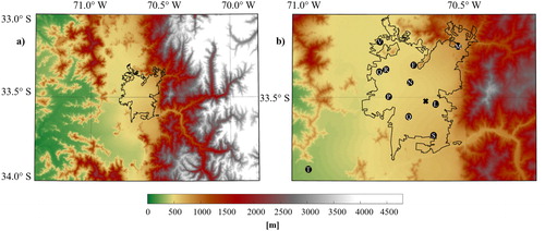
The city of Santiago (33.5S, 70.5 W, 500 m a.s.l.) in Chile is located in a semi-arid basin (annual precipitation ∼300 mm) west of the high Andes, which have an average altitude of 4.5 km, and east of a coastal mountain range with an average altitude of 1500 m a.s.l. Figure 1 shows the location of Santiago and significant topographic features, the air quality monitoring station network of Santiago, and other sites of interest. Santiago has a population of 7.2 million inhabitants and a built area of 776 km² (Gallardo et al., 2018). The climate of Santiago is characterized by the quasi-permanent influence of the subtropical Pacific high, and the intrusion of occasional cold fronts, which bring precipitation in wintertime (Montecinos and Aceituno, 2003). The South Pacific high determines quasi-stagnant anti-cyclonic conditions that are further intensified, especially in fall and winter by the presence of sub-synoptic features known as coastal-lows (Rutllant and Garreaud, 1995; Garreaud et al., 2002). There is a characteristic radiatively driven circulation that defines up-slope south-westerly winds in the afternoons and down-slope north-easterly winds in the night and morning hours, more strongly so in the summer (Saide et al., 2011). These forcings result in marked seasonal changes in maximum daily mixing height with lowest median values in winter (∼200 m) and highest median values in summer (∼800 m) (Muñoz and Undurraga, 2010). The solar radiation minimum occurs in winter (∼ 6.5 kwh/m²/day) and the maximum in summer (∼8.4 kwh/m²/day) (Molina et al., 2017). All these factors result in favourable conditions for the accumulation of pollutants and air pollutant precursors in the cold season (March–August), and photochemical pollution, characterised here by ozone (O₃) and nitrogen dioxide (NO₂), in the warm season (September–February) (Elshorbany, Kleffmann, et al., 2009; Elshorbany et al., 2010; Mazzeo et al., 2018).

Fig. 1. Topographic features affecting Santiago and location of air quality monitoring stations. Also shown is the site (x, San Joaquín) where aerosol speciation was assessed in 2013 by Villalobos et al. (2015). The map on the left (a) shows the location of the city and the topography of the area. The map on the right (b) shows a close-up of the map and the location of the stations in the air quality network of Santiago. Stations are: F (Independencia); L (La Florida); M (Las Condes); N (Parque O’Higgins); O (Pudahuel); P (Cerrillos); Q (El Bosque); R (Cerro Navia); S (Puente Alto); T (Talagante). For instrumentation in the air quality network and other details see Table S1.

According to the latest emission inventory available for Santiago (USACH, 2014), the transportation and residential sectors are dominant sources of primary particles. In this emission inventory, transportation and residential burning contribute 41% and 35% of a total of 5.8 k ton/yr of PM_2.5. Barraza et al. (2017), using receptor modeling techniques, describe the contribution of different sectors to PM_2.5 for the period 1998–2012. During 2011–2012, on an annual basis, they attributed a contribution of 39% to the transportation sector, followed by industrial sources (20%), and the residential sector (18%). Residential sources peak in the cold season explaining ca. 35% of PM_2.5 (Mena-Carrasco et al., 2012; Villalobos et al., 2015; Barraza et al., 2017; Mazzeo et al., 2018).

Barraza et al. (2017), using observational data, evidenced the contribution of “coastal sources”, i.e., a mixture of marine aerosols and industrial sources, explaining roughly 9% of the mass of PM_2.5 measured in downtown Santiago in 2012. They also argue that the mass concentrations associated with that contribution declined over the years, which they attribute to the use of cleaner fuel in the industrial zones on the coast. They characterise the seasonal contribution of this coastal source having its maximum in fall and being non-significant in summer. Furthermore, they identify that “copper smelters” are both a local and remote source. In any case, they see a decreasing contribution from this source in accordance with the enforcement of more strict environmental regulations in Chile. In a recent modeling study, Langner et al. (2020) combined three inventories covering the political regions that are expected to influence Santiago’s air quality, to quantify source contributions to PM_2.5 in Santiago and the region of central Chile. According to their simulations, dominant primary sources in Santiago originate from traffic and machinery, and residential wood burning in the outskirts of Santiago (in the cold season). They found a significant regional background of secondary inorganic aerosols (SIA) of about 5 µg/m³, and a much smaller contribution of secondary organic aerosols (SOA), generally below 1 µg/m³.

Furthermore, modelling the impact assessment of upwind emissions to air quality in the Santiago basin is somehow limited by the fact that Chile does not have a nation-wide, consistent inventory for air quality purposes, which has implied considering either only specific pollutants and sources (Gallardo et al., 2002; Olivares et al., 2002) or a combination of local (city-scale) and global inventories (Mazzeo et al., 2018). Downscaling of global inventories that use generic national statistics mis-represents the relative role of different sources and is not recommended for air quality studies (Huneeus et al., 2020). Also, if local inventories are built using different methodologies and data sources, they may be inconsistent when combined to cover a larger area (Gallardo et al., 2012).

Overall, Langner et al. (2020)´s results are consistent with those of Barraza et al. (2017), in the sense that they both show that the largest contributions to PM_2.5 in Santiago arise from sources and processes within the basin, with background SIA and SOA contributing a smaller – though not negligible – fraction of Santiago’s PM_2.5.

The evolution of air quality in Santiago has been recently described by Gallardo et al. (2018). According to these authors, PM₁₀ (PM_2.5) showed a decline of −22.3 ± 11.4 (–8.42 ± 5.30) µg/m³ per decade in downtown Santiago (Parque O’Higgins station) between 1988 and 2016 (1998 and 2014), despite population growth, city expansion, economic growth, increases in the private vehicular fleet, etc., which reflects the success of policy measures adopted since the early 1990s when democracy was reinstated. Similarly, Barraza et al. (2017) show that PM_2.5 median mass concentrations declined from 33.5 µg/m³ in 1998–1999 to 17.2 µg/m³ in 2011–2012. Attainment plans have been mainly technological (e.g., fuel quality, three-way catalytic converters, diesel particle filters) and operational (e.g. a new transport system, the Transantiago and annual mandatory vehicular inspections). Also, efficient air quality forecasting tools have been implemented, helping to prevent very high pollution events in winter (Saide et al., 2011, 2016). However, despite these efforts, Santiago remains a polluted city regarding ozone and PM_2.5 (Gallardo et al., 2018; Seguel et al., 2020). In fact, we quantify a decadal trend of +1.8 ± 1.3 µg/m³ in PM_2.5 between 2009 and 2018 in downtown Santiago (see Fig. S1 in the supplementary material). Thus, PM_2.5 levels have improved since the early 2000s, yet they still pose severe health risks as well as an increasing trend in Santiago.

Photochemical pollution has not received much attention in terms of new public policy in Santiago since efforts have been greatly devoted to reducing acute particle events in winter (Gallardo et al., 2018). Relatively few studies have addressed photochemical processes (e.g., Rubio et al., 2002; Rappenglück et al., 2005; Elshorbany, Kleffmann, et al., 2009; Elshorbany, Kurtenbach, et al., 2009; Elshorbany et al., 2010; Villena et al., 2011; Seguel et al., 2012, 2013). Also, the characterization of volatile organic compounds is scarce (e.g., Kavouras et al., 1999; Rubio et al., 2006; Préndez et al., 2013; Toro and Seguel, 2015). Furthermore, the maximum daily eight-hour running average of 61 ppbv for ozone is frequently exceeded in Eastern Santiago, particularly at Las Condes station, where ozone hourly mixing ratios can surpass 160 ppbv in summer, and 90 ppbv in winter (Supplement Fig. S2). In Western Santiago at Pudahuel station, ozone is close to compliance, but particle concentrations are often well above annual and daily standards in winter (Supplement Fig. S3). The Metropolitan Region of Santiago has kept its status as a non-attainment area for O₃ according to the latest Attainment Plan for Santiago (Seguel et al., 2020). These high levels of photochemical pollution need further research, and policy action. This is true even if the policy focus remains on aerosols, as secondary aerosols are an important aspect of aerosol pollution (Volkamer et al., 2006; Huang et al., 2014; Zhang et al., 2015).

In this paper, we argue that in addition to the changes mentioned above, the overall result of the atmospheric oxidants, characterised here by the sum of O₃ and NO₂, i.e., O_x=O₃+NO₂ (Guicherit, 1988; Kley et al., 1994; Clapp and Jenkin, 2001), leads to more secondary aerosol formation –both inorganic and organic– and photochemical pollution. To this end, and due to the lack of long-term speciation data for particles, we use an empirical methodology (Chang and Lee, 2007) to estimate the secondary aerosol fraction of PM_2.5 in Santiago.

To the best of our knowledge, this is the first study in Chile assessing long-term (∼20 years) changes in secondary aerosol composition in Chile. Previous studies only characterized short-periods of time (less than a year), without giving further insights in the evolution of aerosol composition in Santiago (e.g., Seguel et al., 2009; Carbone et al., 2013; Villalobos et al., 2015; Tagle et al., 2018). Understanding the secondary fraction of ambient aerosol is not only relevant for understanding photochemical processes (Turpin and Huntzicker, 1995; Turnbull and Harrison, 2000; Rodrı́guez et al., 2002; Na et al., 2004) but also due to the role of secondary pollution in terms of health effects (e.g., Atkinson et al., 2014; Wang et al., 2018), and climate e.g., (Shrivastava et al., 2017; Scott et al., 2018; Tsigaridis and Kanakidou, 2018).

In the next section, we describe the data and methodology used in this paper. Results are presented and discussed thereafter. Summary and conclusions are shown in the final section of the paper.

2. Data and methodology

2.1. Data sources and handling

More than two decades of hourly air quality data are publically available for Santiago and other cities in Chile through a publicly available web site maintained by the Ministry of the Environment of Chile (https://sinca.mma.gob.cl/). The network and the data have been described and assessed elsewhere (e.g., Osses et al., 2013; Henriquez et al., 2015; Toro et al., 2015; Gallardo et al., 2018). The current distribution of monitoring stations in Santiago is shown in Fig. 1. Table S1 in the supplementary material, summarises species and measurement methods, as well as which species are measured in each station. These data have been used to characterise the O_x trends between January 1 of 2001 and December 31 of 2018.

We focus on two urban stations in the Santiago network, namely Pudahuel (33.44S, 70.75 W, 460 m a.s.l) and Las Condes (33.38S, 70.52 W, 712 m a.s.l.), however some results for other stations are shown. Pudahuel and Las Condes have been chosen since they represent very different parts of the city with respect to socioeconomic, emission, atmospheric circulation, and concentration characteristics (e.g., Saide et al., 2011; Gallardo et al., 2012, 2018; Mazzeo et al., 2018; Tagle et al., 2018). Pudahuel, in the west of Santiago and at 460 m a.s.l., is characterised by a low-to-middle class inhabitants, whereas Las Condes, at 795 m. a.s.l., is located in the east of the city, i.e., it is a receptor site, particularly in the afternoon hours, and corresponds to a relatively wealthy part of the city. Also, these stations have long-term O₃ and NO₂ data. Data were downloaded on March 20^th, 2019. Not all data had been subject to an official review, so we applied several quality checks. These quality checks included detection limits of instruments, physical restrictions e.g., (PM_2.5≤ PM₁₀; NO₂≤NO_x-NO); completeness (availability of at least 75$\mathrm{\%}$ of the hourly data for calculating daily averages, and 75% of daily averages for calculating monthly averages); eliminating isolated extremely high hourly values (values over six times the previous or posterior two hours were removed).

Trends in atmospheric aerosols and oxidant levels were calculated, applying the approach used by Duncan et al. (2016) and Lamsal et al. (2015), estimating regression errors according to the method in Tiao et al. (1990). This approach deseasonalises the data series and takes auto-correlation and length of monthly averaged series into consideration. The relationship between O_x and NO_x is used to infer the background ozone at each station (Clapp and Jenkin, 2001), as well as the evolution of this parameter over time. In this case we assume a measurement error of 10% for O_x and NO_x, and apply the error estimated by Neri et al. (1989), which provides a linear regression accounting for errors in the ordinate and abscissa.

2.2. Empirical estimate of secondary aerosols

We use the empirical approach by Chang and Lee (2007), which is based on previous work by various authors (Grosjean, 1989; Kley et al., 1994; Turpin and Huntzicker, 1995; Rodrı́guez et al., 2002; Na et al., 2004), and recently applied by (Jia et al., 2017). In this method, primary particles are estimated based on their correlation with carbon monoxide (CO), and daily ozone maxima (O_{3, max}) are used as a proxy for photochemical activity that is propitious for secondary aerosol formation. Essentially, the better the PM_2.5-to-CO correlation the more primary aerosols there will be, and the higher the ozone levels, the more secondary particles there will be.

The choice of CO as a proxy for PM_2.5 primary sources appears fully justifiable in the case of combustion sources such as transportation and residential heating, which, according to the latest emission inventory for Santiago (USACH, 2014), contribute 76% of the total annual emissions, a fraction largely consistent with elemental composition analyses attributing 57% to these sources (Barraza et al., 2017). The methodology may nevertheless underestimate the contribution of industrial processes, urban dust, and remote sources, including secondary aerosols as highlighted by Langner et al. (2020). Thus, on the one hand, not considering other primary sources in Santiago may lead to an underestimation of primary PM_2.5. On the other hand, SIA or SOA produced outside the Santiago basin may be included as primary PM_2.5. Finally, we are not aware of any recent studies showing long-term changes in aerosol composition or how the relative contribution of sources may have changed between 2012 and the present day. Moreover, one must bear in mind that Chang and Lee (2007) used an empirical estimate, like us, to account for the lack of observations, which are the standard characterisation of the primary and secondary fractions.

2.2.1. Choice of ozone categories

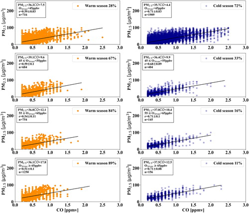
For this methodology, the observational data must be classified according to ozone levels, thus defining when secondary aerosol formation is occurring. An ozone level below which one assumes that there is no significant in-situ secondary aerosol formation, and above which this process is favoured must be identified. Originally, following Chang and Lee (2007), upon inspection of the linearity of the PM_2.5-to-CO relationship shown in Fig. 2, an O_{3, max}=45 ppbv was identified as the limit below which the PM_2.5-to-CO is linear. This selection was supported by an ozone-sonde study that identified 45 ppbv as the upper tier for ozone background in a peri-urban site, upwind from Santiago (Seguel et al., 2013). Furthermore, we distinguished: four categories of data according to different photochemical activity as characterised by O₃ mixing ratios. They are distinguished as low photochemistry with O_{3, max}<45 ppbv, medium photochemistry with 45 ppbv ≤ O_{3, max} ≤ 55 ppbv, medium-to-high with 55 ppbv < O_{3, max}≤ 65 ppbv, and high photochemistry with O_{3, max} >65 ppbv. A statistical analysis of the goodness-of-fit (Wilks, 2011) of the regressions are provided in Fig. 2 in the supplementary material (see Table S2, and Fig. S4).

Fig. 2. Relationship between daily averages of PM_2.5 (in µg/m³) and CO (in ppmv) for Las Condes station in Eastern Santiago, between 2001 and 2018. Data are stratified according to season: warm (September through February), shown in the left panel, and cold (March through August) shown in the right panel. Data are also stratified according to ozone daily maximum range: horizontal panels show the relation for low (a,b), medium (c,d), medium-to-high (e,f), and high (g,h) photochemical activity. The corresponding linear regression lines (shown in black) and correlation factors are also shown, as well as the number of concurrent CO and PM_2.5 measurements (n). The percentage is calculated as the ratio between the cold/warm season points with respect to the total number of data points considered in the regression.

A k-means clustering analysis was performed, aimed at identifying different photochemical regimes considering hourly values of PM_2.5 and CO, and daily maxima of ozone (O_{3, max}). This analysis shows a distinct behaviour between the warm and the cold seasons (see Supplement Figs. S3 and S4). It also identifies a group of data in the warm season with high PM_2.5 when ozone is above ∼65 ppbv, irrespective of CO values. Furthermore, there was a group with PM_2.5 values that rose to above 40 µg/m³ when ozone daily maxima exceeded ca. 45 ppbv. Hence, the clustering analysis supports our choice of ozone categories.

Taking all this into account, “low photochemical activity” was defined as when O_{3, max} was less than 45 ppbv, and there is a linear relationship between PM_2.5 and CO (Fig. 2a, b). When O_{3, max} was above 45 ppbv, the correlation between PM_2.5 and CO weakened, particularly in the warm season, suggesting secondary aerosol formation (Fig. 2g, h).

Finally, beyond statistics, the background O₃ from the intercept of the linear regression between O_x=O₃+NO₂ and NO_x during daytime (Clapp and Jenkin, 2001; Notario et al., 2012) was corroborated, as shown in Fig. 3. Since Las Condes is a receptor site, the corresponding regression intercept is higher than that found at Pudahuel for all seasons. Also, the intercept at Las Condes in the warm season is significantly higher than in the cold season reflecting the intensification of photochemistry with higher temperatures and more solar radiation. Pudahuel, on the other hand, shows no significant difference between the seasons. The latter suggests that Pudahuel behaves as an “urban background site” regarding photochemistry.

Fig. 3. Background oxidant, i.e., O_x=O₃+NO₂, mixing ratios for Pudahuel and Las Condes for the period 2005–2018 when both O₃, NO and NO₂ are available. The upper panels show the daylight hours O_x vs NO_x linear regressions according to Neri et al. (1989) for the cold (blue) and warm (brown) seasons, in Las Condes (left) and Pudahuel (right). The lower panel shows the evolution of the intercept of the linear regressions of each year between 2005 and 2018, for Las Condes (black symbols) and for Pudahuel (grey symbols).

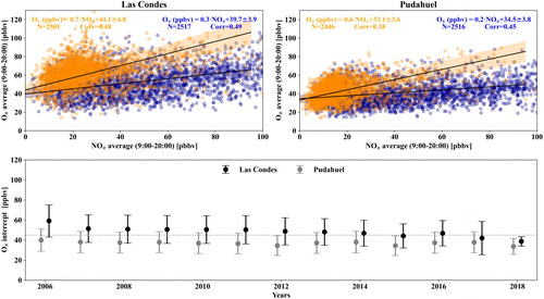
Figure 3 also shows the evolution of the intercept calculated for every year between 2006 and 2018, as well as the 45 ppbv “low photochemistry” level. The figure shows that the 45 ppbv level is generally in the upper (mid-to-lower) range of the Pudahuel (Las Condes) annual intercept values, except in 2018, when it is above both intercept ranges. Thus, choosing a 45 ppbv limit may result in a slight underestimate (overestimate) of the PM_2.5 secondary fraction at Pudahuel (Las Condes), and an underestimate at both stations in 2018. The choice of a 45 ppbv level on an annual basis is, nevertheless, a middle ground choice when using nearly 20 years of data.

2.2.2. Estimating the secondary fraction

Following Chang and Lee (2007), based on the assumption that PM_2.5 and CO under low photochemical activity are only primary, we can estimate the fraction of primary particles in PM_2.5 at a given hour by using the following ratio taken as characteristic of primary emissions: (1) $$(\frac{P{M}_{2.5}}{CO}{)}_{p,L,h}$$(1) where the subscripts p and L stand for primary and low photochemical activity (O_{3, max} <45 ppbv) respectively. The h index indicates hourly data. Thus, the primary PM_2.5 aerosol mass is derived from hourly observations as follows: (2) $$(P{M}_{2.5}{)}_{p,X,h}=(CO{)}_{p,X}(\frac{P{M}_{2.5}}{CO}{)}_{p,L,h}$$(2) where, X = M, MH or H indicate medium, medium-to-high, and high photochemical activity respectively, corresponding to the ranges indicated in Fig. 2. Secondary aerosols are then estimated as the difference between the observed PM_2.5 and the primary aerosols that are calculated as explained above.

3. Results

3.1. Empirical estimates for the annual evolution of secondary aerosols

Using hourly observations of PM_2.5, CO, and O₃, and applying the methodology discussed in Section 2.2, we estimated the primary and secondary fractions of PM_2.5 for Santiago between 2001 and 2018.

3.1.1. Interannual variability

First, we show the interannual variability of secondary fractions on a year-by-year basis, including all daily averages of the hourly secondary fractions every two consecutive years, to assure robust statistics. Figure 4 shows the percentage fraction of PM_2.5 that is of secondary origin at Pudahuel and Las Condes stations for the period 2001–2018, and for the ozone ranges with O_{3, max} above 45 ppbv, i.e., all O_{3, max} categories. If one considers the higher ranges of O_{3, max} the fraction of secondary aerosols increases somewhat, particularly in the warm season when such values are more frequent (see Supplement Fig. S7).

Fig. 4. Evolution of the daily (24 hours) secondary aerosol fraction (in %) as calculated by the methodology by Chang and Lee (2007). The upper (lower) panel shows the results (bars) for Las Condes (Pudahuel) station in Eastern (Western) Santiago, considering O_{3, max} > 45 ppbv. The error range is calculated as the standard deviation of each 2-year average. Results are shown for the whole year (black bars) as well as for the cold (green) and warm (red) seasons.

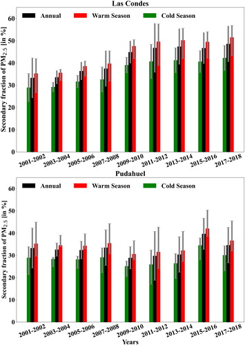
The data shows that trends and contributions of secondary aerosol show a heterogeneous spatial distribution. While in Pudahuel –Western Santiago– this fraction has remained relatively constant varying between 28% and 39% the past 18 years, in Las Condes –Eastern Santiago– the secondary aerosol contribution to PM_2.5 has shown an increasing trend with annual averages rising from roughly 30$\mathrm{\%}$ in the early 2000s to nearly 50$\%$ in 2018 (see Fig. 4). Also, in the warm season there are more secondary aerosols than in the cold season due to higher ozone mixing ratios. In Las Condes, the secondary PM_2.5 fraction starts to surpass the 40% limit in the warm season of 2009. This shift is concurrent with changes in ozone, NO₂ and PM_2.5 trends as presented in Table 1 and Supplementary Figs. S8 and S9. This trend shift in PM_2.5 in downtown Santiago was linked by Barraza et al. (2017) to changes in fleet technology and composition, and the number of vehicles associated to the implementation of the Transantiago, the new combined public transportation system (Muñoz et al., 2014). These changes appear to have affected the photochemistry of Santiago at large, as discussed later.

Table 1. Trends and trend error estimates of O₃, NO₂, O_x, and PM_2.5 observed at Eastern (Las Condes) and Western (Pudahuel) Santiago monitoring stations for different periods, based on monthly mean observations. Data source: http://sinca.mma.gob.cl/. Time series are shown in the supplementary material (Figs. S5 and S6a–f for Las Condes and Pudahuel respectively).

Station/Species	Period
	2001–2008	2009–2018	2001–2018
Eastern Santiago (Las Condes)
O3	−5.1 ± 1.1 (n = 96)	−0.4 ± 1.9 (n = 110)	−1.4 ± 1.7 (n = 206)
NO2	6.2 ± 1.7 (n = 33)	7.3 ± 3.1 (n = 107)	4.2 ± 2.7 (n = 140)
Ox	2.9 ± 1.3 (n = 32)	6.2 ± 3.1 (n = 99)	4.2 ± 1.2 (n = 131)
PM2.5	−3.5 ± 1.2 (n = 93)	2.2 ± 1.4 (n = 117)	−2.6 ± 1.5 (n = 210)
PM2.5 secondary	0.7 ± 0.4 (n = 93)	2.3 ± 0.7 (n = 117)	1.6 ± 0.6 (n = 210)
PM2.5 primary	−3.6 ± 0.7 (n = 93)	0.5 ± 1.4 (n = 117)	−3.8 ± 1.1 (n = 210)
Western Santiago (Pudahuel)
O3	−0.8 ± 0.7 (n = 95)	−4.6 ± 1.0 (n = 110)	−2.7 ± 1.9 (n = 205)
NO2	−3.7 ± 3.1 (n = 33)	1.2 ± 1.8 (n = 105)	1.1 ± 2.3 (n = 138)
Ox	−3.6 ± 1.3 (n = 33)	−3.9 ± 1.6 (n = 97)	−3.7 ± 2.0 (n = 138)
PM2.5	−2.3 ± 2.5 (n = 93)	−2.0 ± 1.9 (n = 118)	−2.7 ± 2.5 (n = 211)
PM2.5 secondary	−0.2 ± 0.8 (n = 93)	0.7 ± 0.2 (n = 118)	−0.9 ± 1.0 (n = 211)
PM2.5 primary	−2.3 ± 2.5 (n = 93)	−2.0 ± 1.9 (n = 118)	−3.5 ± 1.8 (n = 211)

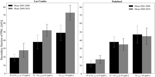
Before proceeding with any further analyses, the consistency of the approach for hourly (not shown) and daily averages of PM_2.5 and CO data was checked, and as expected, the higher the ozone levels, the higher was the secondary aerosol fraction in PM_2.5. This is illustrated in Fig. 5, where the secondary fraction is classified according to ozone ranges and considering two periods (2001–2008 and 2009–2018).

Fig. 5. Average fraction of secondary aerosol (in %) and standard deviation segregated by daily ozone maximum range, and by period, for stations Las Condes (Left panel) and Pudahuel (Right panel). The different time periods considered, i.e., 2001–2008 and 2009–2018, are shown in black and grey, respectively.

3.1.2. Diurnal variability

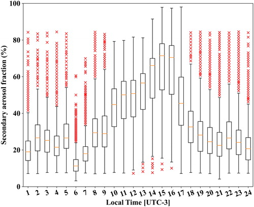
Increased secondary aerosol fractions were estimated in the warm months, and in the afternoon hours, when ozone mixing ratios are at a maximum (see Fig. 6). The results are, again, consistent with the notion that more photochemical activity leads to more secondary aerosol. Nevertheless, it is worth noticing that high ozone events and secondary aerosol formation also occur in the cold season, albeit less frequently.

Fig. 6. Diurnal cycle of secondary aerosol fraction (in %) estimated at Las Condes station for the warm season (September–February) for the period 2001–2018. Data are presented as box plots: the central mark in the box indicates the median of the distribution, the edges of the box are the 25th and 75th percentiles, the whiskers extend to the most extreme data points not considered outliers, and outliers are plotted individually (red crosses). The number of outliers is less than 2% of the points considered in each box. See details in the text.

3.2. Comparison with observations

Our estimates were compared with previous observations of aerosol composition as reported in the literature (Seguel et al., 2009; Carbone et al., 2013; Villalobos et al., 2015; Tagle et al., 2018; Langner et al., 2020). The only study reporting both inorganic and organic fraction of PM_2.5 over several months in 2013 is Villalobos et al. (2015). The corresponding comparison between our estimate for Las Condes and La Florida stations, both in Eastern Santiago, with monthly averaged values from Villalobos et al. (2015) are shown in Fig. 7. La Florida was included because it is the closest station to the site (San Joaquín) where these observations were collected (Cf. Fig. 1).

Fig. 7. Monthly averaged secondary fraction of PM_2.5 (black dotted line) for stations Las Condes (upper panel) and La Florida (lower panel) in Eastern Santiago as estimated using the empirical method (Chang and Lee, 2007). The grey colour indicates the standard deviation of the monthly values calculated over daily averages. The corresponding monthly averaged measured by Villalobos et al. (2015) at San Joaquín near La Florida station are also shown (blue dashed line).

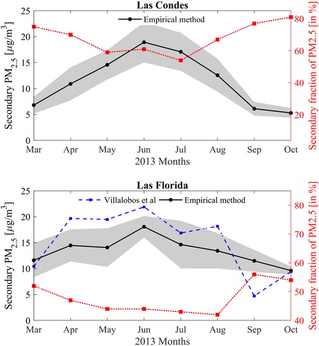
The observations at San Joaquín (Cf. Fig. 1) show highest secondary PM_2.5 in June 2013, and lowest in the transitional months of March and September. This is well captured by the empirical estimate in Eastern Santiago. The values provided by the empirical estimate are nevertheless somewhat lower than the observed values for April through August at La Florida, which is located less than 3 km east of San Joaquín. Las Condes, on the other hand, is nearly 17 km north-east of La Florida and there, the empirical estimate shows similar maximum secondary PM_2.5 in June but with sharper differences among months in the period March–October 2013. This suggests that the formation of secondary aerosols is dependent on local conditions, possibly driven by local photochemistry. In fact, the level of oxidants, here characterised by O_x (see Fig. 3), shows an upwind contribution and a local contribution that varies from site to site (Clapp and Jenkin, 2001).

Both at Las Condes and La Florida, the estimated secondary fraction shows a maximum in the warmer months, and a minimum in the cold months but the seasonal variation is more marked at Las Condes than at La Florida. Also, at Las Condes the secondary fraction is larger (50 to 80%) than at La Florida (40 to 55%). Such differences reflect on the one hand, the heterogeneous distribution of primary PM_2.5 sources, and the prevalent wind conditions at each monitoring station. While the former changes significantly given the uneven socioeconomic characteristics, transportation activity and technology, etc. (e.g., Saide et al., 2011; Gallardo et al., 2012; Mazzeo et al., 2018), the latter is less variable in the daytime due to the marked thermally driven circulation that prevails in Santiago (see Fig. S10). During the night-time, while at La Florida relatively weak downslope winds bring air from the Maipo Valley (SE of Santiago), Las Condes receives air from the Mapocho Valley (NE of Santiago). This may have a differentiation effect in terms of remote influxes of PM_2.5, and issue that requires further investigation.

In Table 2 we summarise the observations of aerosol chemical composition as measured in Santiago from previous studies and compare those with our estimates. Secondary inorganic and secondary aerosol components are indicated when available in the observations. As discussed earlier, Villalobos et al. (2015) found a secondary fraction of ca. 50% over Eastern Santiago (San Joaquín near La Florida station) that compares well with our estimate. In this study, SOA is a slightly greater fraction of PM_2.5 than SIA. Seguel et al. (2009) do not report SIA but they infer a small SOA fraction. Langner et al (2020) also find that SIA much larger than SOA, however their simulations and observations refer mostly to the cold season. Our estimate for concurrent times and sites with the secondary aerosol observations, indicates a secondary fraction between 34 and 50% that is generally larger than the SIA concentrations reported in those studies, leaving the possibility of there being some SOA. However, as our method is based on the measurements of PM_2.5 provided by the air quality monitoring network, which are not the same as those used in aerosol composition measurements, the comparison is not straight forward. Hence, as there are no outstanding differences between the observed values and those estimated with the simple empirical methodology, we deem it as adequate for looking at the long-term evolution of secondary aerosol in Santiago.

Fig. 8. Decadal trends (%) in O₃, NO₂ and O_x=O₃+NO₂ in Santiago for the period 2009–2018. Blurry circles with an asterisk indicate statistically non-significant trends. Trends are calculated over deseasonalized monthly averaged values using the approach by Duncan et al. (2016).

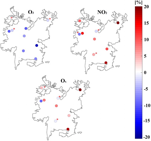
Table 2. Chemical composition of aerosols as measured in Santiago in previous studies. Secondary inorganic (SIA) and organic (SOA) aerosol components are indicated when available. N/A indicates not available. The percentage corresponds to the fraction of total aerosol. We also include our estimate of the secondary fraction (%) and the total PM2.5 mass concentration (calculated as hourly averages over the period) at the closest station.

Location	Date	SIA	SOA	PM2.5	This work		Reference and brief explanation
		[μg/m³] (%)	[μg/m³] (%)	[μg/m³]	Secondary Fraction	PM2.5 [μg/m³]
Las Condes (33.38S, 70.52W)	Feb 2004	N/A	1.3 (4%)	31.0	41%	26.4	Elemental Carbon (EC) tracer method based on background organic carbon (OC) to EC ratios (Seguel et al., 2009)
Pudahuel (33.44S, 70.75W)		N/A	0.3 (1%)	24.0	34%	25.0
San Joaquín (33.49S, 70.62 W)	Mar–Oct 2013	5.63 (23%)	7.58 (30%)	25.3	47%	22.2	The elemental analysis was conducted by X-ray fluorescence/ Source apportionment (Villalobos et al., 2015). Our values at station La Florida, 3 km east from San Joaquín
USACH (33.45S, 70.68 W)	Mar–Jul 2012	9.2 (30%)	N/A	30.3	39%	32.2	Reported measurements in Langner et al. (2020), analogous to Tagle et al. (2018)
	May–Jul 2012	10.6 (29%)	N/A	37.1	34%	35.8
USACH (33.45S, 70.68 W)	Spring 2011	9.9 (34%)	N/A	29.8	36%	19.6	Aerosol Chemical Speciation Monitor (ACSM) (Carbone et al., 2013). Our values at station Parque O'Higgins, ∼ 2 km south east from USACH.
Pudahuel (33.44S, 70.75 W)	Spring 2016	5.8 (30%)	N/A	19.1	41%	15.6	Optical analyser to determine black carbon and Aerosol Chemical Speciation Monitor (ACSM) (Tagle et al., 2018). They report submicron concentrations as seasonal 1-hour averages.
Las Condes (33.38S, 70.52 W)	Spring 2016	7.7 (29%)	N/A	26.9	48%	17.1
Pudahuel (33.44S, 70.75 W)	Winter 2016	11.8 (24%)	N/A	48.3	33%	70.5
Las Condes (33.38S, 70.52 W)	Winter 2016	18.2 (44%)	N/A	41.6	40%	30.4

3.2.1. Consistency with emission inventory

Carbon monoxide emissions are dominated (>90%) by the transportation sector in Santiago (Gallardo et al., 2012; USACH, 2014). For PM_2.5 emissions, the transportation sector is also very relevant (∼40%) but industrial, residential and to some extent remote sources are also significant (Mena-Carrasco et al., 2012; USACH, 2014; Barraza et al., 2017; Langner et al., 2020). To see whether we might over or underestimate the secondary fraction, we used the same approach as Chang and Lee (2007), i.e., we checked the PM_2.5-to-CO ratio for transportation in the inventory (USACH, 2014), finding a value of 0.019. This value is generally lower than the median observed ratios (see Supplement Fig. S11). Hence, the observed ratios used to estimate the primary fraction in the methodology may in general lead to an underestimate of the secondary fraction.

3.3. Changes in oxidative capacity

To understand the trend in secondary aerosol contribution to PM_2.5 and its differences between Eastern and Western Santiago, we examine the changes in the O₃ and NO₂ mixing ratios as indicators of changes in photochemical activity. The oxidative capacity of the atmosphere is largely determined by the presence of the hydroxyl radical (OH) in the daytime (Thompson, 1992; Atkinson and Arey, 2003; Prinn, 2003). Due to the lack of direct measurements of OH, the ratio between volatile organic compounds and nitrogen oxides (VOC/NO_x) has been frequently used as an indicator of the ozone formation regime, i.e., whether the OH radical is being eliminated through termination reactions or is being optimally regenerated through VOC oxidation that results in ozone formation and other secondary products (Fujita et al., 2003). Therefore, insights from O₃ and NO_x behaviour can be drawn in the absence of VOC observations.

Here we discuss trends in oxidative capacity, as expressed in O_x=O₃+NO₂ and as observed at eight out of 11 stations in Santiago for the period 2001–2018 (see Fig. 8). Trends are also calculated for deseasonalized monthly averaged values. Ozone shows declining trends at all stations, with the highest negative trend observed at La Florida station (33.44S, 70.59 W, 590 m a.s.l) in the east of Santiago. Increasing trends in NO₂ are noted at all sites, except at Pudahuel, where a small but not significant decline (<5%) is observed, possibly linked to titration by primary nitric oxide emissions. Overall, the increase in NO₂ results in statistically significant growth in O_x, particularly over Eastern Santiago. Hence, NO₂ is playing a key role in Santiago's photochemistry, which in turn impacts secondary aerosol formation. Nitrogen dioxide is in itself a concern regarding human health (Latza et al., 2009). A positive trend in NO₂ over Santiago has been already pointed out by Duncan et al. (2016). Since NO₂ is transformed into ozone downwind from high NO_x emission areas, increasing trends in this pollutant are seen as higher ozone mixing ratios in and downwind of Santiago (Seguel et al., 2020), with detrimental consequences on human health (e.g., Héroux et al., 2015; Fleming et al., 2018), vegetation and agriculture (Mauzerall and Wang, 2001; Ainsworth, 2017; Seguel et al., 2020), and regional climate (Monks et al., 2015; Von Schneidemesser et al., 2015).

In Table 1 we summarize trends in O_x, O₃, NO₂ and PM_2.5 –including the primary and secondary fractions – for Pudahuel and Las Condes for various periods. Over the period 2009–2018, the O_x trend is 6.2 ± 3.1 ppbv/decade, which is more than twice the value in the previous period (2.9 ± 1.3 ppbv/decade, i.e., between 2001 and 2008) in Eastern Santiago (Las Condes). The growth in O_x between 2001 and 2018 (2009–2018) is largely explained by an increase of 4.2 ± 2.7 ppbv/decade (7.3 ± 3.1 ppbv/decade) in NO₂. This is consistent with the trend changes discussed in the previous section, and with the increase in NO₂ observed from space for the period 2004–2014 (Duncan et al., 2016) where a trend of 30 ± 17% was calculated, compared to our estimate of 16 ± 9% between 2004 and 2014, which is encouragingly consistent in light of the very different types of data and methods used. Also, the number of vehicles circulating in Santiago has markedly increased in later years: in 2007 there were 1.2 million vehicles, and in 2018 more than 2 million vehicles (INE, 2018). However, current emission estimates for mobile sources do not show increasing NO_x emissions, due to the growing share of stringent technologies in the vehicle fleet (Tolvett-Caro et al., 2016). Since traffic constitutes ca. 80% of NO_x emissions according to the most recent official inventory for Santiago (USACH, 2014), it is difficult to reconcile the observed increase in NO₂ mixing ratios with current emission estimates. However, abatement technologies may in fact induce an increase in the fraction of NO₂ emitted from vehicles, particularly but not solely using diesel (Carslaw, 2005; Alvarez et al., 2008; Carslaw et al., 2011). Moreover, the effects of the deterioration of catalytic converts (Corvalán and Vargas, 2003) and shortcomings in inspection systems cannot be ruled out. Explaining the discrepancies between emission estimates and observed NO₂ trends goes beyond the scope of this work but it is worth further investigation, particularly in light of trends observed in Europe and elsewhere (Grange et al., 2017).

A better understanding of NO_x trends and partitioning between NO and NO₂ is critical since high mixing ratios of NO₂ have direct implications on the oxidative capacity (Saiz-Lopez et al., 2017). At low VOC/NO_x ratios, with relatively high NO_x mixing ratios, NO₂ reacts with OH radicals forming nitric acid, instead of being photolyzed to lead to O₃ formation. In addition, less OH radicals are available to initiate the oxidation of VOCs that will lead to NO₂ formation without O₃ consumption. Thus, under this regime, the ozone formation is inhibited (Finlayson-Pitts and Pitts, 2000; Im and Kanakidou, 2012). This phenomenon has been observed mainly during weekdays in Santiago (Seguel et al., 2012) where they show that at weekends, the drop in NO_x favours an O₃ increase. For example, in the warm season 2017–2018, the average mixing ratio of ozone was 28% higher at the weekend (Sunday) compared to on workdays (Monday–Thursday) (see Fig. S12 in the Supplement). Conversely, average mixing ratios of NO and NO₂ were respectively 46% and 32% less at the weekend (Sunday) with respect to workdays (Monday–Thursday). This behaviour suggests a VOC–limited ozone formation regime in Eastern Santiago, e.g., (Fujita et al., 2003).

The PM_2.5 data in Las Condes show a positive trend of 2.2 ± 1.4 µg/m³/decade between 2009 and 2018. Here, the growth in PM_2.5 between 2009 and 2018 is largely driven by the growth of the secondary fraction. In fact, over the whole period (2001–2018) the secondary fraction has shown an increasing trend. Over Western Santiago, the PM_2.5 trend remains negative for the whole period, but it is increasingly less negative. Here, there is also positive trend in secondary aerosol between 2009 and 2018. Thus, if the trend in O_x remains positive overall in the city, we can expect a growth of the secondary fraction here as well, and thus a shift towards increasing PM_2.5. Hence it is of paramount importance to pay attention to photochemical pollution, adopting adequate mitigation strategies, which in turn will require a more process-oriented monitoring, including measuring VOCs.

Changes in oxidative capacity in urban environments have been reported for several cities (Sheehy et al., 2010; Volkamer et al., 2010; Pollack et al., 2013; Saiz-Lopez et al., 2017). These studies show how sensitive the oxidative capacity is to emission regulations of anthropogenic NO_x and VOCs, and how abatement strategies vary depending on location, regional transport patterns, and the sources involved (e.g., Parrish et al., 2011, 2016; Hallquist et al., 2016).

Changes in oxidative capacity may be further enhanced by the drying and warming trends observed and projected for Central Chile (Boisier et al., 2018). This may affect ozone pollution in two major ways. On the one hand, relatively high temperatures accelerate chemical reactions leading to ozone formation (e.g., Sillman and Samson, 1995; Walcek and Yuan, 1995; Bloomer et al., 2009). On the other hand, biogenic VOC emissions may increase with warming temperatures leading to more ozone formation (e.g., Atkinson and Arey, 2003; Pacifico et al., 2012). Also, heat waves can lead to increased photochemical production (Langner et al., 2012; Hou and Wu, 2016; Seguel et al., 2020). Hence, over time it will be harder to attain ozone standards, i.e., a climate penalty (Jacob and Winner, 2009)

4. Summary and conclusions

In this work, we used an empirical methodology to estimate the secondary aerosol fraction –both organic and inorganic– of PM_2.5 in Santiago. Changes in oxidative capacity were characterized by in situ measurements of O_x= O₃+NO₂. Our results show an increasing O_x, driven by NO₂ growth, that leads to secondary aerosol formation. Fully inhalable particles show a positive trend PM_2.5 over Eastern Santiago, particularly in the period 2009–2018, and this increase is dominated by the growth of the secondary fraction. We present results for Las Condes station in Eastern Santiago, where the contribution of secondary particles grew from ca. 35% in 2007 to ca. 50% in 2018. Our estimate is partially corroborated by a 7-months in situ measurements of chemical composition of PM_2.5 in Santiago in 2013 (Villalobos et al., 2015), as well as other observations and a recent modeling study. Over Western Santiago, the contribution to PM_2.5 of secondary aerosol remains below 40% for the same period, with the secondary fraction also increasing. Both the available observations and the empirical estimate suggest a strong spatial heterogeneity in photochemical activity in Santiago, highlighting the need for further photochemical studies.

In situ data show an increasing trend in the sum of O₃ and NO₂ (O_x) mixing ratios whose overall result is impacting the oxidative capacity at all stations except at Pudahuel where a minor decline is found due to decreasing ozone, possibly titrated by NO emissions. The increase in O_x is marked over Eastern Santiago between 2009 and 2018 (6.2 ± 3.1 ppbv/decade). This positive trend in O_x is driven by the increase in NO₂ (7.3 ± 3.1 ppbv/decade) in the same period, which is playing a key role in Santiago's photochemistry, determining an increase in the secondary fraction of PM_2.5. The increasing trend of NO₂ is also seen from space (Duncan et al., 2016), and it may be associated with the growth of the vehicular fleet that has nearly doubled since 2007. However, current estimates of the evolution of traffic emissions do not show such a trend. Further research regarding this mismatch is necessary but it may also originate in photochemistry changes.

The increasing role of secondary aerosols in PM_2.5 shown in this study, and the evidence of a more oxidizing atmosphere, make it necessary to pay more attention to photochemical pollution than has been the case so far in Santiago, and in Central Chile at large. To this end, more regular speciation studies of aerosols, as well as more systematic assessments of ozone precursors, including volatile organic compounds is required. Such data will improve our ability to constrain model simulations, and provide the foundation for more efficient pollution control, through new curbing measures with an explicit focus on photochemical pollution in Santiagós (and elsewhere in Central Chile’s) attainment plans. When doing so, it will be necessary to adopt a regional scale perspective considering upwind sources of photochemical pollutants and downwind impacts on vegetation and agriculture, as well as on human health and climate.

Addressing photochemical pollution, including secondary aerosols is crucial for Santiago, and most probably for central Chile at large. Particularly, when Central Chile is facing the consequences of a changing climate that is leading to drier conditions and warmer temperatures in Central Chile. We must be careful in choosing adequate adaptation and mitigation measures, and to that end we will need more process-oriented measurements and monitoring. In the meantime, we expect to carry out further research using a multi-model approach to characterize photochemical pollution and secondary aerosols.

Acknowledgements

We are grateful for the comments from two anonymous reviewers.

Disclosure statement

No potential conflict of interest was reported by the authors.

Supplemental data

Supplemental data for this article can be accessed here.

Additional information

Funding

This work was conducted within the framework of the Center for Climate and Resilient Research (FONDAP 15110009), and the PAPILA (Prediction of Air Pollution in Latin America and the Caribbean) project (ID: 777544, H2020-EU.1.3.3.). NH and LG also acknowledge FONDECYT project 1181139. NH was also supported by the Research and Innovation programs under grant agreement no 870301 (AQ-WATCH) and by the MAP-AQ, which is an IGAC and WMO sponsored activity. MK acknowledges support from the General Secretariat for Research and Technology in Greece and the University of Crete (project ID 4162).

References

- Ainsworth, E. A. 2017. Understanding and improving global crop response to ozone pollution. Plant J. 90, 886–897. doi:10.1111/tpj.13298
- Alvarez, R., Weilenmann, M. and Favez, J. Y. 2008. Evidence of increased mass fraction of NO2 within real-world NOx emissions of modern light vehicles - derived from a reliable online measuring method. Atmos. Environ. 42, 4699–4707. doi:10.1016/j.atmosenv.2008.01.046
- Atkinson, R. and Arey, J. 2003. Atmospheric degradation of volatile organic compounds. Chem. Rev. 103, 4605–4638. doi:10.1021/cr0206420
- Atkinson, R. W., Kang, S., Anderson, H. R., Mills, I. C. and Walton, H. A. 2014. Epidemiological time series studies of PM2.5 and daily mortality and hospital admissions: A systematic review and meta-analysis. Thorax 69, 660–665. doi:10.1136/thoraxjnl-2013-204492
- Barraza, F., Lambert, F., Jorquera, H., Villalobos, A. M. and Gallardo, L. 2017. Temporal evolution of main ambient PM2.5 sources in Santiago, Chile, from 1998 to 2012. Atmos. Chem. Phys. 17, 10093–10107. doi:10.5194/acp-17-10093-2017
- Bloomer, B. J., Stehr, J. W., Piety, C. A., Salawitch, R. J. and Dickerson, R. R. 2009. Observed relationships of ozone air pollution with temperature and emissions. Geophys. Res. Lett. 36, L09803.
- Boisier, J. P., Alvarez-Garreton, C., Cordero, R. R., Damiani, A., Gallardo, L. and co-authors. 2018. Anthropogenic drying in central-southern Chile evidenced by long-term observations and climate model simulations. Elementa 6, 74.
- Carbone, S., Saarikoski, S., Frey, A., Reyes, F., Reyes, P. and co-authors. 2013. Chemical characterization of submicron Aerosol particles in Santiago de Chile. Aerosol. Air Qual. Res. 13, 462–473. doi:10.4209/aaqr.2012.10.0261
- Carslaw, D. C. 2005. Evidence of an increasing NO2/NOX emissions ratio from road traffic emissions. Atmos. Environ. 39, 4793–4802. doi:10.1016/j.atmosenv.2005.06.023
- Carslaw, D. C., Beevers, S. D., Tate, J. E., Westmoreland, E. J. and Williams, M. L. 2011. Recent evidence concerning higher NOx emissions from passenger cars and light duty vehicles. Atmos. Environ. 45, 7053–7063. doi:10.1016/j.atmosenv.2011.09.063
- Chang, S. C. and Lee, C. T. 2007. Secondary aerosol formation through photochemical reactions estimated by using air quality monitoring data in Taipei City from 1994 to 2003. Atmos. Environ. 41, 4002–4017. doi:10.1016/j.atmosenv.2007.01.040
- Clapp, L. J. and Jenkin, M. E. 2001. Analysis of the relationship between ambient levels of O3, NO2 and NO as a function of NOx in the UK. Atmos. Environ. 35, 6391–6405. doi:10.1016/S1352-2310(01)00378-8
- Corvalán, R. M. and Vargas, D. 2003. Experimental analysis of emission deterioration factors for light duty catalytic vehicles Case study: Santiago, Chile. Transp. Res. Part D: Transp. Environ. 8, 315–322. doi:10.1016/S1361-9209(03)00018-X
- Duncan, B. N., Lamsal, L. N., Thompson, A. M., Yoshida, Y., Lu, Z. and co-authors. 2016. A space-based, high-resolution view of notable changes in urban NOx pollution around the world (2005–2014. J. Geophys. Res. Atmos. 121, 976–996. doi:10.1002/2015JD024121
- Elshorbany, Y. F., Kleffmann, J., Kurtenbach, R., Lissi, E., Rubio, M. and co-authors. 2010. Seasonal dependence of the oxidation capacity of the city of Santiago de Chile. Atmos. Environ. 44, 5383–5394. doi:10.1016/j.atmosenv.2009.08.036
- Elshorbany, Y. F., Kleffmann, J., Kurtenbach, R., Rubio, M., Lissi, E. and co-authors. 2009. Summertime photochemical ozone formation in Santiago, Chile. Atmos. Environ. 43, 6398–6407. doi:10.1016/j.atmosenv.2009.08.047
- Elshorbany, Y. F., Kurtenbach, R., Wiesen, P., Lissi, E., Rubio, M. and co-authors. 2009. Oxidation capacity of the city air of Santiago, Chile. Atmos. Chem. Phys. 9, 2257–2273. doi:10.5194/acp-9-2257-2009
- Finlayson-Pitts, B. J. and Pitts, J. N. 2000. Overview of the chemistry of polluted and remote atmospheres. In: Chemistry of the Upper and Lower Atmosphere. Elsevier, San Diego, pp. 1–14. doi:https://doi.org/10.1016/B978-012257060-5/50003-4
- Fleming, Z. L., Doherty, R. M., Von Schneidemesser, E., Malley, C. S., Cooper, O. R. and co-authors. 2018. Tropospheric ozone assessment report: Present-day ozone distribution and trends relevant to human health. Elem. Sci. Anth. 6, 12. doi:10.1525/elementa.273
- Fujita, E. M., Stockwell, W. R., Campbell, D. E., Keislar, R. E. and Lawson, D. R. 2003. Evolution of the magnitude and spatial extent of the weekend ozone effect in California's South Coast Air Basin, 1981–2000. J. Air Waste Manag. Assoc. 53, 802–815. doi:10.1080/10473289.2003.10466225
- Gallardo, L., Barraza, F., Ceballos, A., Galleguillos, M., Huneeus, N. and co-authors. 2018. Evolution of air quality in Santiago: The role of mobility and lessons from the science-policy interface. Elementa 6, 38.
- Gallardo, L., Escribano, J., Dawidowski, L., Rojas, N., de Fátima Andrade, M. and co-authors. 2012. Evaluation of vehicle emission inventories for carbon monoxide and nitrogen oxides for Bogotá, Buenos Aires, Santiago, and São Paulo. Atmos. Environ. 47, 12–19. doi:10.1016/j.atmosenv.2011.11.051
- Gallardo, L., Olivares, G., Langner, J. and Aarhus, B. 2002. Coastal lows and sulfur air pollution in Central Chile. Atmos. Environ. 36, 3829–3841. doi:10.1016/S1352-2310(02)00285-6
- Garreaud, R. D., Rutllant, J. A. and Fuenzalida, H. 2002. Coastal lows along the subtropical west coast of South America: Mean structure and evolution. Mon. Wea. Rev. 130, 75–88. doi:10.1175/1520-0493(2002)130<0075:CLATSW>2.0.CO;2
- Grange, S. K., Lewis, A. C., Moller, S. J. and Carslaw, D. C. 2017. Lower vehicular primary emissions of NO2 in Europe than assumed in policy projections. Nat. Geosci. 10, 914–918. doi:10.1038/s41561-017-0009-0
- Grosjean, D. 1989. Organic acids in Southern California Air: Ambient concentrations, mobile source emissions. Environ. Sci. Technol. 23, 1506–1514. doi:10.1021/es00070a009
- Guicherit, R. 1988. Ozone on an urban and regional scale. In: Tropospheric Ozone. Springer, Netherlands, pp. 49–62. doi:https://doi.org/10.1007/978-94-009-2913-5_3
- Hallquist, M., Munthe, J., Hu, M., Wang, T., Chan, C. K. and co-authors. 2016. Photochemical smog in China: Scientific challenges and implications for air-quality policies. Natl. Sci. Rev. 3, 401–403. doi:10.1093/nsr/nww080
- Henriquez, A., Osses, A., Gallardo, L. and Resquin, M. D. 2015. Analysis and optimal design of air quality monitoring networks using a variational approach. Tellus, Ser. B: Chem. Phys. Meteorol. 67, 25385. doi:10.3402/tellusb.v67.25385
- Héroux, M. E., Anderson, H. R., Atkinson, R., Brunekreef, B., Cohen, A. and co-authors. 2015. Quantifying the health impacts of ambient air pollutants: recommendations of a WHO/Europe project. Int. J. Public Health 60, 619–627. doi:10.1007/s00038-015-0690-y
- Hou, P. and Wu, S. 2016. Long-term changes in extreme air pollution meteorology and the implications for air quality. Sci. Rep. 6, 23792. doi:10.1038/srep23792
- Huang, R. J., Zhang, Y., Bozzetti, C., Ho, K. F., Cao, J. J. and co-authors. 2014. High secondary aerosol contribution to particulate pollution during haze events in China. Nature 514, 218–222. doi:10.1038/nature13774
- Huneeus, N., Denier van der Gon, H., Castesana, P., Menares, C., Granier, C. and co-authors. 2020. Evaluation of anthropogenic air pollutant emission inventories for South America at national and city scale. Atmos. Environ. 235, 117606. doi:10.1016/j.atmosenv.2020.117606
- Im, U. and Kanakidou, M. 2012. Impacts of East Mediterranean megacity emissions on air quality. Atmos. Chem. Phys. 12, 6335–6355. doi:10.5194/acp-12-6335-2012
- INE. 2018. Tabulado de vehículos en circulación 2018. docs/default-source/parque-de-vehiculos/cuadros-estadisticos/resultados/cifras-2018.xlsx?sfvrsn=ced9a153_4
- Jacob, D. J. and Winner, D. A. 2009. Effect of climate change on air quality. Atmos. Environ. 43, 51–63. doi:10.1016/j.atmosenv.2008.09.051
- Jia, M., Zhao, T., Cheng, X., Gong, S., Zhang, X. and co-authors. 2017. Inverse relations of PM2.5 and O3 in air compound pollution between cold and hot seasons over an urban area of East China. Atmosphere 8, 59. doi:10.3390/atmos8030059
- Kavouras, I. G., Lawrence, J., Koutrakis, P., Stephanou, E. G. and Oyola, P. 1999. Measurement of particulate aliphatic and polynuclear aromatic hydrocarbons in Santiago de Chile: Source reconciliation and evaluation of sampling artifacts. Atmos. Environ. 33, 4977–4986. doi:10.1016/S1352-2310(99)00281-2
- Kley, D., Geiss, H. and Mohnen, V. A. 1994. Tropospheric ozone at elevated sites and precursor emissions in the United States and Europe. Atmos. Environ. 28, 149–158. doi:10.1016/1352-2310(94)90030-2
- Lamsal, L. N., Duncan, B. N., Yoshida, Y., Krotkov, N. A., Pickering, K. E. and co-authors. 2015. U.S. NO2 trends (2005–2013): EPA Air Quality System (AQS) data versus improved observations from the Ozone Monitoring Instrument (OMI). Atmos. Environ. 110, 130–143. doi:10.1016/j.atmosenv.2015.03.055
- Langner, J., Engardt, M., Baklanov, A., Christensen, J. H., Gauss, M. and co-authors. 2012. A multi-model study of impacts of climate change on surface ozone in Europe. Atmos. Chem. Phys. 12, 10423–10440. doi:10.5194/acp-12-10423-2012
- Langner, J., Gidhagen, L., Bergström, R., Gramsch, E., Oyola, P. and co-authors. 2020. Model-simulated source contributions to PM2.5 in Santiago and the central region of Chile. Aerosol. Air Qual. Res. 20, 1111–1126. doi:10.4209/aaqr.2019.08.0374
- Latza, U., Gerdes, S. and Baur, X. 2009. Effects of nitrogen dioxide on human health: Systematic review of experimental and epidemiological studies conducted between 2002 and 2006. Int. J. Hyg. Environ. Health 212, 271–287. doi:10.1016/j.ijheh.2008.06.003
- Mauzerall, D. L. and Wang, X. 2001. Protecting agricultural crops from the effects of tropospheric ozone exposure: Reconciling science and standard setting in the United States. Annu. Rev. Energy Environ. 26, 237–268. doi:10.1146/annurev.energy.26.1.237
- Mazzeo, A., Huneeus, N., Ordoñez, C., Orfanoz-Cheuquelaf, A., Menut, L. and co-authors. 2018. Impact of residential combustion and transport emissions on air pollution in Santiago during winter. Atmos. Environ. 190, 195–208. doi:10.1016/j.atmosenv.2018.06.043
- Mena-Carrasco, M., Oliva, E., Saide, P., Spak, S. N., de la Maza, C. and co-authors. 2012. Estimating the health benefits from natural gas use in transport and heating in Santiago, Chile. Sci. Total Environ. 429, 257–265. doi:10.1016/j.scitotenv.2012.04.037
- Molina, A., Falvey, M. and Rondanelli, R. 2017. A solar radiation database for Chile. Sci. Rep. 7, 1–11.
- Monks, P. S., Archibald, A. T., Colette, A., Cooper, O., Coyle, M. and co-authors. 2015. Tropospheric ozone and its precursors from the urban to the global scale from air quality to short-lived climate forcer. Atmos. Chem. Phys. 15, 8889–8973. doi:10.5194/acp-15-8889-2015
- Montecinos, A. and Aceituno, P. 2003. Seasonality of the ENSO-related rainfall variability in Central Chile and associated circulation anomalies. J. Clim. 16, 281–296. doi:10.1175/1520-0442(2003)016<0281:SOTERR>2.0.CO;2
- Muñoz, J. C., Batarce, M. and Hidalgo, D. 2014. Transantiago, five years after its launch. Res. Transp. Econ. 48, 184–193. doi:10.1016/j.retrec.2014.09.041
- Muñoz, R. C. and Undurraga, A. A. 2010. Daytime mixed layer over the Santiago Basin: Description of two years of observations with a lidar ceilometer. J. Appl. Meteorol. Climatol. 49, 1728–1741. doi:10.1175/2010JAMC2347.1
- Na, K., Sawant, A. A., Song, C. and Cocker, D. R. 2004. Primary and secondary carbonaceous species in the atmosphere of Western Riverside County, California. Atmos. Environ. 38, 1345–1355. doi:10.1016/j.atmosenv.2003.11.023
- Neri, F., Saitta, G. and Chiofalo, S. 1989. An accurate and straightforward approach to line regression analysis of error-affected experimental data. J. Phys. E: Sci. Instrum. 22, 215–217. doi:10.1088/0022-3735/22/4/002
- Notario, A., Bravo, I., Adame, J. A., Díaz-de-Mera, Y., Aranda, A. and co-authors. 2012. Analysis of NO, NO 2, NO x, O 3 and oxidant (OX = O 3 + NO 2) levels measured in a metropolitan area in the southwest of Iberian Peninsula. Atmos. Res. 104–105, 217–226. doi:10.1016/j.atmosres.2011.10.008
- Olivares, G., Gallardo, L., Langner, J. and Aarhus, B. 2002. Regional dispersion of oxidized sulfur in Central Chile. Atmos. Environ. 36, 3819–3828. doi:10.1016/S1352-2310(02)00286-8
- Osses, A., Gallardo, L. and Faundez, T. 2013. Analysis and evolution of air quality monitoring networks using combined statistical information indexes. Tellus, Ser. B: Chem. Phys. Meteorol. 65, 19822–19817. doi:10.3402/tellusb.v65i0.19822
- Pacifico, F., Folberth, G. A., Jones, C. D., Harrison, S. P. and Collins, W. J. 2012. Sensitivity of biogenic isoprene emissions to past, present, and future environmental conditions and implications for atmospheric chemistry. J. Geophys. Res. 117.
- Parrish, D. D., Singh, H. B., Molina, L. and Madronich, S. 2011. Air quality progress in North American megacities: A review. Atmos. Environ. 45, 7015–7025. doi:10.1016/j.atmosenv.2011.09.039
- Parrish, D. D., Xu, J., Croes, B. and Shao, M. 2016. Air quality improvement in Los Angeles—perspectives for developing cities. Front. Environ. Sci. Eng. 10, 11. doi:10.1007/s11783-016-0859-5
- Pollack, I. B., Ryerson, T. B., Trainer, M., Neuman, J. A., Roberts, J. M. and co-authors. 2013. Trends in ozone, its precursors, and related secondary oxidation products in Los Angeles, California: A synthesis of measurements from 1960 to 2010. J. Geophys. Res. Atmos. 118, 5893–5911. doi:10.1002/jgrd.50472
- Préndez, M., Carvajal, V., Corada, K., Morales, J., Alarcón, F. and co-authors. 2013. Biogenic volatile organic compounds from the urban forest of the Metropolitan Region, Chile. Environ. Pollut. 183, 143–150. doi:10.1016/j.envpol.2013.04.003
- Prinn, R. G. 2003. The cleansing capacity of the atmosphere. Annu. Rev. Environ. Resour. 28, 29–57. doi:10.1146/annurev.energy.28.011503.163425
- Rappenglück, B., Schmitz, R., Bauerfeind, M., Cereceda-Balic, F., Von Baer, D. and co-authors. 2005. An urban photochemistry study in Santiago de Chile. Atmos. Environ. 39, 2913–2931. doi:10.1016/j.atmosenv.2004.12.049
- Rodrı́guez, S., Querol, X., Alastuey, A., and Mantilla, E. 2002. Origin of high summer PM10 and TSP concentrations at rural sites in Eastern Spain. Atmos. Environ. 36, 3101–3112. doi:10.1016/S1352-2310(02)00256-X
- Rubio, M. A., Lissi, E. and Villena, G. 2002. Nitrite in rain and dew in Santiago city, Chile. Its possible impact on the early morning start of the photochemical smog. Atmos. Environ. 36, 293–297. doi:10.1016/S1352-2310(01)00356-9
- Rubio, M. A., Zamorano, N., Lissi, E., Rojas, A., Gutiérrez, L. and co-authors. 2006. Volatile carbonylic compounds in downtown Santiago, Chile. Chemosphere 62, 1011–1020. doi:10.1016/j.chemosphere.2005.06.022
- Rutllant, J. and Garreaud, R. 1995. Meteorological air pollution potential for Santiago, Chile: Towards an objective episode forecasting. Environ. Monit. Assess. 34, 223–244. doi:10.1007/BF00554796
- Saide, P. E., Carmichael, G. R., Spak, S. N., Gallardo, L., Osses, A. E. and co-authors. 2011. Forecasting urban PM10 and PM2.5 pollution episodes in very stable nocturnal conditions and complex terrain using WRF-Chem CO tracer model. Atmos. Environ. 45, 2769–2780. doi:10.1016/j.atmosenv.2011.02.001
- Saide, P. E., Mena-Carrasco, M., Tolvett, S., Hernandez, P. and Carmichael, G. R. 2016. Air quality forecasting for winter-time PM2.5episodes occurring in multiple cities in central and southern Chile. J. Geophys. Res. Atmos. 121, 558–575. doi:10.1002/2015JD023949
- Saiz-Lopez, A., Borge, R., Notario, A., Adame, J. A., La Paz, D. D. and co-authors. 2017. Unexpected increase in the oxidation capacity of the urban atmosphere of Madrid, Spain. Sci. Rep. 7, 45956. doi:10.1038/srep45956
- Scott, C. E., Arnold, S. R., Monks, S. A., Asmi, A., Paasonen, P. and co-authors. 2018. Substantial large-scale feedbacks between natural aerosols and climate. Nat. Geosci. 11, 44–48. doi:10.1038/s41561-017-0020-5
- Seguel, R. J., Mancilla, C. A., Rondanelli, R., Leiva, M. A. and Morales, R. G. E. 2013. Ozone distribution in the lower troposphere over complex terrain in Central Chile. J. Geophys. Res. Atmos. 118, 2966–2980. doi:10.1002/jgrd.50293
- Seguel, R. J., Morales, R. G. E. and Leiva, M. A. 2009. Estimations of primary and secondary organic carbon formation in PM2.5 aerosols of Santiago City, Chile. Atmos. Environ. 43, 2125–2131. doi:10.1016/j.atmosenv.2009.01.029
- Seguel, R. J., Morales S, R. G. E. and Leiva G, M. A. 2012. Ozone weekend effect in Santiago, Chile. Environ. Pollut. 162, 72–79. doi:10.1016/j.envpol.2011.10.019
- Seguel, R. J., Gallardo, L., Fleming, Z. L. and Landeros, S. 2020. Two decades of ozone standard exceedances in Santiago de Chile. Air Qual. Atmos. Health 13, 593–605. doi:10.1007/s11869-020-00822-w
- Sheehy, P. M., Volkamer, R., Molina, L. T. and Molina, M. J. 2010. Oxidative capacity of the Mexico City atmosphere-Part 2: A ROx radical cycling perspective. Atmos. Chem. Phys. 10, 6993–7008. doi:10.5194/acp-10-6993-2010
- Shrivastava, M., Cappa, C. D., Fan, J., Goldstein, A. H., Guenther, A. B. and co-authors. 2017. Recent advances in understanding secondary organic aerosol: Implications for global climate forcing. Rev. Geophys. 55, 509–559. doi:10.1002/2016RG000540
- Sillman, S. and Samson, P. J. 1995. Impact of temperature on oxidant photochemistry in urban polluted rural and remote environments. J. Geophys. Res. 100, 11497–11508. doi:10.1029/94JD02146
- Tagle, M., Reyes, F., Vásquez, Y., Carbone, S., Saarikoski, S. and co-authors. 2018. Spatiotemporal variation in composition of submicron particles in Santiago Metropolitan Region, Chile. Front. Environ. Sci. 6, 27. doi:10.3389/fenvs.2018.00027
- Thompson, A. M. 1992. The oxidizing capacity of the earth's atmosphere: probable past and future changes. Science 256, 1157–1165. doi:10.1126/science.256.5060.1157
- Tiao, G. C., Reinsel, G. C., Xu, D., Pedrick, J. H., Zhu, X. and co-authors. 1990. Effects of autocorrelation and temporal sampling schemes on estimates of trend and spatial correlation. J. Geophys. Res. 95, 20507. doi:10.1029/JD095iD12p20507
- Tolvett-Caro, S., Henríquez, P. and Osses, M. 2016. Análisis de variables significativas para la generación deun inventario de emisiones de fuentes móviles y su proyección. Ingeniare. Rev. chil. Ing. 24, 32–39. doi:10.4067/S0718-33052016000500005
- Toro, R. A., Campos, C., Molina, C., Morales, R. G. E. and Leiva-Guzmán, M. A. 2015. Accuracy and reliability of Chile's National Air Quality Information System for measuring particulate matter: Beta attenuation monitoring issue. Environ. Int. 82, 101–109. doi:10.1016/j.envint.2015.02.009
- Toro, R. and Seguel, R. J. 2015. Ozone, nitrogen oxides, and volatile organic compounds in a central zone of Chile. Air Qual. Atmos. Health 8, 545–557. doi:10.1007/s11869-014-0306-3
- Tsigaridis, K. and Kanakidou, M. 2018. The present and future of secondary organic aerosol direct forcing on climate. Curr. Clim. Change Rep. 4, 84–98. doi:10.1007/s40641-018-0092-3
- Turnbull, A. B. and Harrison, R. M. 2000. Major component contributions to PM10 composition in the UK atmosphere. Atmos. Environ. 34, 3129–3137. doi:10.1016/S1352-2310(99)00441-0
- Turpin, B. J. and Huntzicker, J. J. 1995. Identification of secondary organic aerosol episodes and quantitation of primary and secondary organic aerosol concentrations during SCAQS. Atmos. Environ. 29, 3527–3544. doi:10.1016/1352-2310(94)00276-Q
- USACH. 2014. Actualización y sistematización del inventario de emisiones de contaminantes atmosféricos en la Región Metropolitana. http://metadatos.mma.gob.cl/sinia/articles-56914_Inf_Inventarios_FINAL.pdf
- Villalobos, A. M., Barraza, F., Jorquera, H. and Schauer, J. J. 2015. Chemical speciation and source apportionment of fine particulate matter in Santiago, Chile, 2013. Sci. Total Environ. 512–513, 133–142. doi:10.1016/j.scitotenv.2015.01.006
- Villena, G., Kleffmann, J., Kurtenbach, R., Wiesen, P., Lissi, E. and co-authors. 2011. Vertical gradients of HONO, NOx and O3 in Santiago de Chile. Atmos. Environ. 45, 3867–3873. doi:10.1016/j.atmosenv.2011.01.073
- Volkamer, R., Sheehy, P., Molina, L. T. and Molina, M. J. 2010. Oxidative capacity of the Mexico City atmosphere-Part 1: A radical source perspective. Atmos. Chem. Phys. 10, 6969–6991. doi:10.5194/acp-10-6969-2010
- Volkamer, R., Jimenez, J. L., San Martini, F., Dzepina, K., Zhang, Q. and co-authors. 2006. Secondary organic aerosol formation from anthropogenic air pollution: Rapid and higher than expected. Geophys. Res. Lett. 33, L17811. doi:10.1029/2006GL026899
- Von Schneidemesser, E., Monks, P. S., Allan, J. D., Bruhwiler, L., Forster, P. and co-authors. 2015. Chemistry and the linkages between air quality and climate change. Chem. Rev. 115, 3856–3897. doi:10.1021/acs.chemrev.5b00089
- Walcek, C. J. and Yuan, H. H. 1995. Calculated influence of temperature-related factors on ozone formation rates in the lower troposphere. J. Appl. Meteor. 34, 1056–1069. doi:10.1175/1520-0450(1995)034<1056:CIOTRF>2.0.CO;2
- Wang, S., Ye, J., Soong, R., Wu, B., Yu, L. and co-authors. 2018. Relationship between chemical composition and oxidative potential of secondary organic aerosol from polycyclic aromatic hydrocarbons. Atmos. Chem. Phys. 18, 3987–4003. doi:10.5194/acp-18-3987-2018
- Wilks, D. S. 2011. Statistical Methods in the Atmospheric Sciences. Vol. 100, Academic press, San Diego.
- Zhang, R., Wang, G., Guo, S., Zamora, M. L., Ying, Q. and co-authors. 2015. Formation of urban fine particulate matter. Chem. Rev. 115, 3803–3855. doi:10.1021/acs.chemrev.5b00067