
 ?Mathematical formulae have been encoded as MathML and are displayed in this HTML version using MathJax in order to improve their display. Uncheck the box to turn MathJax off. This feature requires Javascript. Click on a formula to zoom.
Abstract
This study aims at estimating errors to be accounted for in atmospheric inversions of methane (CH4) emissions at the European scale. Four types of errors are estimated in the concentration space over the model domain and at selected measurement sites. Furthermore, errors in emission inventories are estimated at country and source sector scales. A technically ready method is used, which is implemented by running a set of simulations of hourly CH4 mixing ratios for 2015 using two area-limited transport models at three horizontal resolutions with multiple data sets of emissions and boundary and initial conditions as inputs. The obtained error estimates provide insights into how these errors could be treated in an inverse modelling system for inverting CH4 emissions over Europe. The main results show that sources of transport errors may better be controlled alongside the emissions, which differs from usual inversion practices. The average total concentration error is estimated at 29 ppb. The assessed error of total CH4 emissions is 22% and emission errors are heterogeneous at sector (23–49%) and country scales (16–124%), with largest errors occurring in the waste sector due to uncertainties in activity data and emission factors and in Finland due to uncertainties in natural wetland emissions.
1. Introduction
Methane (CH4) contributed up to 11% to the total greenhouse gas (GHG) emissions of the European Union (EU) in 2017 (EEA, Citation2019), after carbon dioxide (79%). In Europe, CH4 is released to the atmosphere by a variety of anthropogenic (more than 80%) and natural (20%) sources (Saunois et al., Citation2016a, Citation2016b). Anthropogenic CH4 mainly originates from the activity of anaerobic bacteria in waste water treatment, landfills and agriculture, mainly through manure management and enteric fermentation of ruminants. Anthropogenic CH4 is also released during fossil fuel extraction, production and distribution, non-industrial combustion (e.g. heating), the use of biofuel, as well as through rice cultivation, biomass burning from agricultural activities and the treatment of agricultural waste. The largest anthropogenic emission sources in the EU are enteric fermentation, manure management and anaerobic waste treatment, accounting for ∼54% of the total anthropogenic sources in 2017 (EEA, Citation2019). Natural sources include methanogenesis in natural wetlands mostly, and to a lesser extent CH4 release in natural gas seeps and by wildfires, through incomplete combustion of the biomass.
Due to CH4’s relatively short atmospheric lifetime of 8–10 years (IPCC, 2013), it is a good target for short-term climate change mitigation. In order to design efficient mitigation strategies, it is necessary to have an advanced understanding on the magnitudes, trends, as well as spatial, temporal and sector distributions of CH4 emissions at the relevant space and time scales. Emissions are defined by activity data and emission factors. The first term refers to anthropogenic socio-economic activities causing emissions, while the second term quantifies sources or sinks per unit of activity (IPCC, Citation2006). Emissions are primarily estimated and characterised by the so-called bottom-up approaches; (i) aggregating socio-economic statistical information in the case of anthropogenic emission inventories (e.g. Kuenen et al., Citation2014), (ii) using process-based numerical models calibrated with local-scale measurements and lab experiments (e.g. Ringeval et al., Citation2010) or (iii) upscaling local models and measurements (e.g. Peltola et al., 2019). However, the large variety of anthropogenic sources associated with high heterogeneity, both in space and time, of their activity data and emission factors leads to imperfect knowledge. All emission data sets have significant but ill-quantified uncertainties, of which the statistical characterisation is particularly difficult (Jonas et al., Citation2011).
An alternative to bottom-up approaches is proposed by top-down atmospheric inversions. The aim of such an approach is to reduce uncertainties on existing emission data sets. They are built to optimally merge atmospheric measurements, numerical modelling of atmospheric transport and chemistry and prior knowledge on emissions. Atmospheric inversions commonly apply Bayesian inversion methods (Tarantola, Citation2005) using bottom-up emission data sets as prior knowledge and assimilating atmospheric mixing ratio data in a chemistry–transport model (CTM) to update this prior knowledge into an optimised posterior emission estimate. In principle, the Bayesian framework makes it possible to obtain the information about the emissions contained in the misfits between the model simulations and the measurements from the other sources of errors, assuming that the statistics of the different types of errors are correctly characterised. Misfits between model simulations and measurements originate from (i) errors in measurements (instrument precision and accuracy), (ii) uncertainties in the chosen prior emission inventory, (iii) projection of emissions to the CTM’s grid, (iv) representativity of simulated mixing ratios in a model grid cell compared to measurements, which can generally be viewed as representative of a point (for in situ measurements) or a line (for remote-sensing data), compared to the typical spatial and temporal resolution of CTMs, (v) boundary conditions used in the CTM for the case of regional CTMs with limited-area domains of simulation, (vi) uncertainties in the modelling of the transport in the CTM itself (discretisation and numerical solving of continuous equations, physical parameterisations and simplifications, uncertainties in the meteorological forcing), as well as (vii) aggregation errors, which are due to the spatial and temporal resolutions of the inversion, which are different from (usually coarser than) the spatial and temporal resolutions of the CTM.
To date, atmospheric studies for the inversion of CH4 emissions use configurations which have been specifically adapted to each inversion system and inverse problem to be solved (e.g. Bergamaschi et al., Citation2005, 2018; Thompson et al., Citation2015; Henne et al., Citation2016; Tsuruta et al., 2019; Wang et al., Citation2019.) In particular, uncertainties in inverse systems are based on approximations, past experience and expert knowledge, which can be biased towards including some specific error-generating processes and ignoring others, for example, taking into account errors due to the vertical mixing in the model and not the errors due to the representation of sub-grid-scale processes. Recent studies have proposed automatic methods representing uncertainties in inversion systems in a more comprehensive way (e.g. Ganesan et al., Citation2014; Berchet et al., Citation2015; Lunt et al., Citation2016; Pison et al., Citation2018; McNorton et al., Citation2020). These studies are based on Monte Carlo approach, systematic exploration of possible uncertainties and/or objective analysis of available data to estimate uncertainties. They primarily optimise the uncertainties in all sources of model-data misfits along with the posterior emissions and uncertainties. Still, underlying assumptions are strong (such as structure of errors and their correlation) and methods are computationally very expensive, making their application hard to replicate, especially for high dimensional problems with emissions at high spatial and temporal resolutions and with large amounts of observations to assimilate.
The replicability and operationality of the uncertainty assessment is especially critical in the field of regional atmospheric inversions of CH4 emissions, with high pressure to deliver reliable results to policy makers in the framework of the Paris Agreement. As the volume of observations will further increase (Bousquet et al., Citation2018; Hu et al., Citation2018; Varon et al., Citation2019), our capability of manually attributing uncertainties will be more and more compromised. Indeed, in the EU, the increasing availability of continuous in situ observations (mainly in the ICOS network, https://www.icos-cp.eu/), of ground-based remote-sensing data (for example, total columns in Wunch et al., Citation2019) and of high-resolution satellite products, makes it necessary to build generic and efficient tools to consistently quantify uncertainties.
In this study, our aim is to obtain uncertainty estimates, which can be used in the framework of inversions of CH4 emissions in Europe by assimilating in situ measurements from surface stations. To obtain these uncertainty estimates, we use a methodology that is computationally inexpensive, easy to reproduce and to update. Easy updating makes it possible to compute improved estimates by including new data products (e.g. new prior emission inventories, meteorology products at high resolutions), covering extended measurement periods, taking into account new measurement sites or large-size data sets (e.g. satellite data). The uncertainty estimates obtained here should help setting-up inversions by providing insights on (i) how to account for sources of errors that are not emission related (e.g. transport with the CTM parameterizations and discretization) and (ii) how to specify error statistics (magnitude, temporal and spatial patterns of errors). The uncertainty estimates are computed at the CTM’s grid resolution and at hourly scales, which are the finest targeted resolution for the foreseen inversions. The spatial and temporal scales targeted by the inversion can also be coarser than the CTM’s: in Europe, a primary target for CH4 could be estimates of emissions at country scale per sector per year or per month.
Following Wang et al. (Citation2017), we base our error analysis and practical implementation on comparisons between simulation outputs and in situ measurements of CH4 mixing ratios, as generated from an ensemble of model simulations. The ensemble of simulations covers the year 2015 and is based on available tools: three inventories of European anthropogenic CH4 emissions, three data sets of natural wetland CH4 emissions, two CTMs with three different horizontal resolutions and two sets of lateral boundary conditions (LBCs). The data sets and the models are described in Section 2. The methodology to compute error estimates is explained in Section 3, where we analyse the magnitude of errors and investigate to what extend they are correlated in time and space. The results are presented and discussed in Section 4, with emphasis on the relations between the different errors. Finally, Section 5 concludes about possible error characterisations and ranges and ways to use these results in atmospheric inversions of European CH4 emissions.
2. Data and model description
2.1. Measurements
In this study, focussed on the year 2015, we use hourly atmospheric measurements of CH4 mixing ratios for at least six months in the year. We originally choose 2015 for the analysis as a large number of measurements are available for this year, used to compare simulation outputs to measurements for choosing the appropriate model layer (see Section 3.2). The selected 31 measurement sites in Europe are listed in and their locations are shown in .
Fig. 1. Locations of the 31 selected measurement sites (with at least six months of data available for 2015, see details in ). Blue triangles indicate mountain sites, green diamonds coastal sites and orange circles indicate ‘other’ sites that are not included in the first two categories.
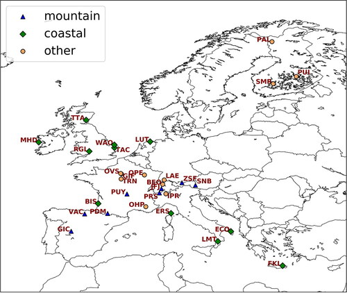
Table 1. Total and sectoral emissions [Tg CH4 year−1] of the TNO-MACC_III, EDGAR v4.3.2 and ECLIPSE V5a anthropogenic inventories in our European domain.
In order to identify links between error statistics and locations and surrounding topography of the measurement sites, we group the measurement sites in three categories: mountain sites, coastal sites and other sites (in most cases, tall towers at rural sites in a relatively flat environment). When a measurement site provides several sampling heights, we use the highest level to limit the effects of local emissions. That, combined with poorly resolved vertical transport near the surface, may lead to biased inversions (Broquet et al., Citation2011).
2.2. Emissions
Three annual anthropogenic gridded emission inventories are used: the TNO-MACC_III (Kuenen et al., Citation2014), the EDGAR v4.3.2 (Janssens-Maenhout et al., Citation2019) and the ECLIPSE V5a (Stohl et al., 2015). At the start of this study, the inventories did not include the year 2015 so that we use the emissions from the most recent year available in each inventory ().
Table 2. Set-ups and input data for the atmospheric chemistry–transport models CHIMERE and LOTOS-EUROS for the simulations in 2015.
For this study, CH4 emissions are grouped into Selected Nomenclature for Air Pollution (SNAP) level-1 sectors to have a common ground for the three inventories, as they use different classifications. In our European domain, agriculture (SNAP 10) is the main emitting sector, followed by the waste sector (SNAP 9). Other relevant emission sources for CH4 are non-industrial combustion plants (SNAP 2) and the production, extraction and distribution of fossil fuels (SNAP 5). The latter two were added into one category that is named ‘fossil fuel related emissions’ hereafter (). The total anthropogenic emissions in EDGAR v4.3.2 are up to 20% larger than in TNO-MACC_III and ECLIPSE V5a but the relative contributions of the three main sectors are very similar across the inventories (). The agriculture sector dominates (about 39–46% of the total CH4 emissions). In this sector, emissions in EDGAR v4.3.2 and TNO-MACC_III are large over Brittany in France, the BENELUX and some Eastern European countries (e.g. Romania, Belarus), while emissions in ECLIPSE V5a are larger than those of EDGAR v4.3.2 and TNO-MACC_III over the Po Valley and generally in Italy. For the waste sector, ECLIPSE V5a generally attributes larger emissions in most countries, while EDGAR v4.3.2 and TNO-MACC_III are large in some individual grid cells. For the fossil fuel related emissions, the largest differences between the three inventories exist over the North Sea and the Ukraine, where the emissions in ECLIPSE V5a are larger than those of the other two inventories.
Furthermore, we use three data sets of natural CH4 emissions to characterise errors from wetland emissions: ORCHIDEE-WET (Ringeval et al., Citation2011), CLASS-CTEM (Arora et al., Citation2018) and JULES (Hayman et al., Citation2014). Even though these process models provide wetland CH4 emissions on a monthly time scale, we use yearly emissions to stay consistent with the choice of anthropogenic emissions (). The sum of ORCHIDEE-WET emissions (7.8 Tg CH4 year−1) over the domain is more than twice as high as that of CLASS-CTEM (3.7 Tg CH4 year−1) and JULES (3.2 Tg CH4 year−1). The top panel of shows the averaged spatial distribution of the total and sectoral emissions for both anthropogenic and natural sources.
Fig. 2. Average (top, in kg m–2 s–1) and standard deviations (SDs, bottom, in kg m−2 s−1) of yearly CH4 emissions from the anthropogenic and natural data sets : total, three main anthropogenic emission sectors and natural wetland emissions (see Section 2.2 for definition).
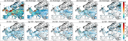
Table 3. Simulations performed with the set-ups of the two chemistry–transport models (CTMs) described in .
2.3. Chemistry–transport models
We use two regional CTMs: CHIMERE (Menut et al., Citation2013; Mailler et al., Citation2017) driven by the system PYVAR (Fortems-Cheiney et al., Citation2019) and LOTOS-EUROS (Manders et al., Citation2017) in a European domain covering [31.5°–74°] in latitude and [−15°–35°] in longitude (). The main characteristics of the set-up of the two models can be found in . The meteorological data used to drive both models are obtained from the European Centre for Medium-Range Weather Forecast (ECMWF) operational forecast product. For the CHIMERE simulations, the boundary and initial concentrations of CH4 are taken either from the analysis and forecasting system developed in the Monitoring Atmospheric Composition and Climate (MACC) project (Marécal et al., 2015) or are pre-optimized LBCs. The pre-optimized LBCs are 4D fields of CH4 concentrations resulting from the inversion by Bousquet et al. (Citation2006), using the global scale Laboratoire de Météorologie Dynamique (LMDz) model (Hourdin et al., Citation2006). The most recent available year from this inversion system is 2010, which we use to provide large-scale patterns and seasonal cycles at the boundaries of our domain for 2015. The CH4 boundary and initial conditions of the LOTOS-EUROS model are taken from the CAMS CH4 reanalysis product (Segers and Houweling, Citation2017). The global concentration fields and meteorological products were interpolated to our models’ resolutions both spatially and temporally.
3. Methodology
3.1. Definition of error sources
We study five errors, described below; one of them is in the emission space and four are in the concentration space:
Error in the emission space:
called hereafter the prior error, which is the error of the emissions in the inventories and process models, particularly due to the spatial distribution of the emissions at the sector and country scales. This error source includes the errors due to the projection of the inventories on the model’s grid and due to the use of different methodology, socio-economic input data and products used for the spatial distribution of emissions in various inventories. The inventories use the E-PRTR database (http://prtr.ec.europa.eu/) for the location of facilities but when no information is found on specific sources, internal databases or other proxies, such as rural or urban population, are used. For example, for the spatial distribution of landfills, EDGAR v4.3.2 uses the E-PRTR database, while TNO-MACC_III makes use of E-PRTR and rural population density. The temporal distribution of
Errors in the concentration space:
As the air masses in the analysed limited-area domain change in approximately 10–14 days and this study focuses on errors near the surface during only one year, which is shorter than the atmospheric lifetime of CH4, errors due to the representation of atmospheric sink processes in the two CTMs are not considered here. Furthermore, this list of errors does not include the aggregation error described in Wang et al. (Citation2017), which is based on Kaminski et al. (Citation2001) and Bocquet et al. (Citation2011). This error is linked to the inversion targeting emissions at a resolution coarser than the CTM’s resolution. To our knowledge, inversion systems do not use the CTM’s native spatio-temporal resolution as a target resolution. In many cases, the CTM’s grid cells are grouped into coarser spatial structures (e.g. national or regional groups) and in most cases, the temporal profiles of emissions are grouped by time periods (from a few hours to days or even years), below which a constant profile is kept throughout the inversion procedure. Inversions with the capability to handle large control vectors, like variational inversions, often control the emissions at a resolution close to that of the transport model (e.g. Broquet et al., Citation2011; Fortems-Cheiney et al., Citation2012), at least spatially. In that case, covers most of the aggregation error. In contrast, for inversions handling low resolution control vectors (e.g. Pison et al., Citation2018), like when using analytical inversion systems, the aggregation error can dominate over many other type of errors (Wang et al., Citation2017). Here, considering our future use of a variational inverse modelling system in which all spatial and temporal scales can be targeted (from the grid-cell and hourly scales to the whole domain and period of interest), we do not further investigate the aggregation error. Our aim is to estimate the dominant contributions to the total transport model and prior errors in order to propose a lower bound for uncertainties and consistent structures of errors.
To evaluate whether an atmospheric inversion is relevant to tackle the targeted CH4 emissions, we compare the magnitudes and structures of
and
to
The relation of
to the other errors in the concentration space is valuable as
contains the expected signal from emissions in the simulated mixing ratios. Several cases are possible:
errors have similar structures and some errors are of the same magnitude as
errors have similar structures and some errors are large compared to
3.2. Estimates of the representation error the transport error the transported-emission error and the background error from simulated CH4 mixing ratios
Following Wang et al. (Citation2017), from the available modelling components (), a total of 11 CHIMERE and three LOTOS-EUROS simulations are run as listed in . In each grid cell c, one estimate of a given for
consists of a time-series of hourly differences between two simulations,
and ψ, of CH4 concentrations which differ by only one aspect:
(1)
(1)
with H an ensemble of hours among all the 8760 h in 2015.
The 14 simulations available are grouped to compute:
Three estimates of
Three estimates of
Three estimates of
One estimate of
As this study is a first step towards regional inversion using real in situ observations, all estimates of errors are also calculated in the grid cells matching the horizontal and vertical location of existing measurements in Europe (see ). To determine the model layer that best fits the height of the measurements for each site, the root mean square error (RMSE) between measured and simulated hourly mixing ratios from 2015 was computed for all the model layers; the layer with the lowest RMSE was then taken to compute error estimates. As CHIMERE uses hybrid σ pressure coordinates that feature small variations of a few metres over time, seasonal effects on the model layer selection are likely negligible. Note that choosing another layer than the one with the lowest RMSE would lead to an increase of the errors in the concentration space.
3.3. Metrics characterising errors
To be able to summarise estimates of error time-series, we define aggregated metrics used later in Section 4. The chosen metrics are the bias (even though bias can be negative or positive, here we are interested only in the magnitude of it), the standard deviation of errors, the spatial correlation of errors as well as the temporal correlation of errors on a given sub-sample H of hours in 2015 (see details on the choice of H in Section 3.4).
For every estimate of a given error
we compute the bias
and the standard deviation
as:
(2)
(2)
with Card(H) being the size of the sample H.
The spatial correlations of an estimate of a given error
are obtained from the bias-corrected correlations for pairs of grid cells
):
(3)
(3)
The correlations are represented as the average of all correlations from all possible pairs for a given distance interval (Section 4.2.4):
(4)
(4)
The temporal auto-correlation R for a given temporal delay k (with unit days) is computed as follows:
(5)
(5)
In most inversion studies, the temporal correlation of errors is assumed to follow an exponential decay. In our case, the auto-correlations quickly decrease before converging to zero but do not necessarily closely follow an exponential decay. Nevertheless, for a simple representation of the temporal correlation, we take the time after which the auto-correlation drops below
For better readability, the spatial distribution of the metric of a given error is not displayed for all possible estimates (e.g. for all pairs of inventories). Instead, we show the average of the metric of interest on all estimates of the error (one for
and three for all other errors, as detailed in Section 3.2) in Sections 3.4, 4.2.1–4.2.3.
3.4. Temporal sampling of error time series
To investigate whether a diurnal cycle is present in the error metrics, we compute the estimates of
for eight sub-samples Wj of simulated hourly concentrations over 3-h long time-windows j:
(6)
(6)
To detect whether there is a period in the day which is more favourable for assimilating observations on regional scale, we compute the ratios of the averages of and
with respect to
for each time-window j, in each grid cell c:
(7)
(7)
We subsequently determine the minimum and maximum of for each
to signal the time-window for which the ratio of errors to
is the smallest. These values are shown and the results described for the locations c of the measurement sites in in Section S3 of the Supplementary material. The results differ from the choice generally made in inversions, based on expert knowledge, to select only afternoon observations for non-mountain sites to limit the impact of poorly-modelled shallow planetary boundary layer (PBL) during the night and early morning. Indeed, the vertical mixing and its impact on the diurnal cycle of mixing ratios are a significant source of error in CTMs (Dabberdt et al., Citation2004; Locatelli et al., 2015; Koffi et al., Citation2016). However, both CTMs in this study use ECMWF data so that errors on the vertical mixing likely follow the same diurnal pattern. It is therefore not possible here to go further in the analysis of the impact of the errors on the vertical mixing at the sub-diurnal scale. In order to stay compatible with the usual choice of afternoon observations for non-mountain sites, in the following, we compute
in each grid cell c from simulated hourly concentrations between 13 h and 17 h UTC included. For mountain sites, we take the simulated hourly concentrations between 00 h and 04 h UTC included. The sample of hourly concentrations H to compute error metrics has then
elements. Our computation of the transport error thus focuses on the horizontal aspect, rather than the vertical one.
3.5. Indicators of characteristics
As the horizontal resolutions of the emission inventories differ, the emissions are spatially interpolated onto the model grids with conserving at least 99% of the mass. The consistency of the spatial distributions of the inventories is represented through the average and standard deviation (SD) of CH4 emissions per sector s in each grid cell c ():
(8)
(8)
(9)
(9)
with fXY the annual emissions from EDGAR v4.3.2 (XY = ED), TNO-MACC_III (XY = TM) and ECLIPSE V5a (XY = EC).
To investigate whether the prior error for a given sector includes spatial correlations, and, if so, whether these correlations can be represented with correlation lengths, the correlations of the
for the three main anthropogenic sectors s are computed (Section 4.1.2). The correlations between sectors are investigated at the European and country scales. All correlations are analysed for significance and are considered significant when the p value is
0.01. At the European scale, the correlations between sectors (hereafter named ‘cross-sector correlations’) are computed. For each pair of sectors (s1, s2), the two sets of three maps of differences in emissions for this sector are used, that is, the series consisting of the list of differences between pairs of inventories, in all grid cells c of the European domain:
(10)
(10)
(11)
(11)
The same method is applied for the natural wetland emission sector. The cross-sector correlations are then represented as a matrix (Section 4.1.3).
To enable the computation of the correlations between two sectors (s1, s2) and between two countries, the correlations between sectors and between countries (hereafter named ‘cross-sector cross-country correlations’) are obtained from two series which describe the 78 possible pairs of countries among 13 selected countries (as defined in ):
(12)
(12)
(13)
(13)
(14)
(14)
Table 4 Standard deviation (SD) relative to the average (%) between the three anthropogenic and natural data sets for selected countries.
The cross-sector cross-country correlations are then represented as a matrix (Section 4.1.3). Contrary to a classical correlation matrix representation, in which only pairs of sectors or pairs of countries are taken into account, the diagonal terms of the matrices in Section 4.1.3 are not equal to 1 as they represent the average correlation between pairs of countries for given sectors and are therefore always smaller than 1.
An inter-annual analysis of is not possible here as the CH4 emissions in the inventories used for this study do not vary within the year. Finally, the uncertainties of the above elements, associated to the three spatially distributed emission inventories, are evaluated by comparison to the total UNFCCC national estimates and estimates from top-down (TD) studies (Section 4.1.4).
4. Results and discussion
4.1. Prior emission uncertainties
4.1.1. Absolute values of
Some studies assume to be homogeneous over the whole domain or per land-use categories, for example, Bergamaschi et al. (Citation2015) with 500% uncertainty in monthly emissions (in their free inversion setting), Tsuruta et al. (2017) with 80% over land and Thompson et al. (Citation2017) with 50% for total emissions in the high northern latitudes. With the inventories used here, the total emissions SD is 22% and
depends on the location and emission sector, as shown by the large SDs (up to 5
10−9 kg m−2 s−1) for waste in almost all countries, for fossil fuel related sectors in some countries only (e.g. the United Kingdom, the Netherlands), for wetlands mainly in Finland, compared to low values for agriculture in almost all countries (). The emissions in the three anthropogenic inventories differ mostly in the waste and the fossil fuel related sectors, with SDs of 58–122% and 35–124% at the national scale in the 13 selected countries (). This can be explained by the different distributions of area and point sources used for these two sectors in the three inventories. In case of wetland emissions, the SDs range between 66% and 101%, which leads to a mean SD for all 13 countries almost as high as in the waste sector (top panel of ). The SDs are lowest in the agriculture sector with values <58%.
The main hot-spots and high-emitting zones could be assumed to be often better known and therefore better located and specified in the inventories. This is the case for high-emitting zones such as the Netherlands or Brittany in France (), where the emissions are mainly due to the agricultural sector (): the spatial patterns of the three inventories are consistent (SDs < 1.5 10−10 kg m−2 s−1, ). Nevertheless, some high-emitting zones or hot-spots are not represented consistently in all three inventories: for example, the off-shore fossil fuel sector in the North Sea ().
Differences between emission inventories are also found in low emitting areas around the coasts (). With differences between emissions over land and sea being large, the effect of different horizontal resolutions becomes distinct at the coasts. With a CTM horizontal resolution lower than that of the inventory, land based emissions are attributed to grid cells encompassing actually land and sea areas. This problem is smaller with higher CTM horizontal resolutions. In general, the approach used for the spatial projection of emissions onto the CTM’s grid impacts the patterns in the interpolated field (conservation of the mass over particular land-use categories for example) so that the interpolation method itself leads to errors. These discrepancies are a source of errors that impact specifically the assimilation of data from coastal measurement sites and need to be addressed in each system.
4.1.2. Spatial correlations in
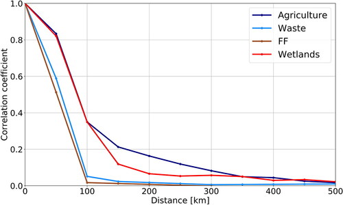
The spatial correlations of the prior emission errors () indicate that an exponential decay function with a correlation length of 100–150 km could be used to model the errors for agriculture and wetlands. For the waste sector and the fossil fuel related sectors, considering that the size of the model grid cells is approximately 50 km
50 km, we assume that spatial correlations can be neglected. Tsuruta et al. (2019) and Bousquet et al. (Citation2011) (inversion INV1) assumed that the errors in emissions
are spatially uncorrelated, which is in agreement with our analysis for the fossil fuel related sectors. In the study of Bergamaschi et al. (Citation2015) (inversion S1), uncertainties of 100% per grid cell and month and spatial correlation scale lengths of 200 km are applied to individual emission sectors. Compared to this setting, our analysis results in a lower average uncertainty and comparable spatial correlation lengths for agriculture and waste. Theoretically, higher uncertainties and lower spatial correlation lengths give more freedom for the inversion to optimise emissions.
Fig. 3. Spatial correlation lengths of the prior errors for the agriculture, waste, fossil fuel (FF) related sectors and wetlands (see Section 2.2 for definition) per grid cell at the horizontal resolution.
4.1.3. Cross-sector and cross-sector cross-country correlations in
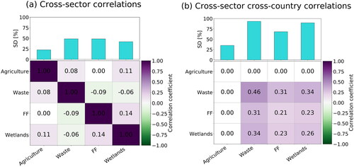
Cross-sector correlations in over the whole domain are presented in . These correlations are computed with a good level of statistical significance (p value <0.01) and are very weak (r < 0.14), reflecting the overall independence of the sectoral emissions in the bottom-up inventories. We also compute cross-country cross-sector correlations () for a subset of 13 countries (see country list in ). The agriculture sector is correlated with no other sectors, which is consistent with the cross-sector correlations over the whole domain. However, the fossil fuel and waste sector exhibit non-negligible cross-country and cross-sector correlations (r = 0.31). These small correlations are likely indirect effects of spatial correlations embedded when building the bottom-up inventories, for example when using proxies such as population density for various sectors.
Fig. 4. Correlations (colour matrices): cross-sector correlations over the European domain (left) and cross-sector cross-country correlations for 13 selected countries (right, see for list). White = correlation not significant, green = negative correlation, violet = positive correlation. The matching standard deviations (SD, in % of the average) are given in the top bar charts.
4.1.4. National-scale uncertainties: comparison to estimates from other studies
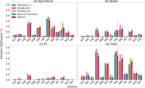
National average emissions of the three anthropogenic gridded inventories and uncertainties estimated in this study are compared to emissions and uncertainties from the UNFCCC national inventory reports (NIR) for the selected 13 countries (). Compared to the NIRs, average emissions of the three anthropogenic gridded inventories are for most countries underestimated in the agriculture sector but overestimated in the waste and fossil fuel related sectors. However, the average country totals of the emissions of the three gridded inventories are still in the range of the NIR uncertainties, which is expected as they are constructed using similar information as the NIRs. Furthermore, the uncertainties in the NIRs are highest in the waste sector for most countries, in agreement with our estimated uncertainties. This suggests that the current knowledge of the activity data and emission factors of the waste emission sector remains less complete than that of the agriculture and fossil fuel related sectors. To deal with the large temporal and spatial variability of the emissions in the waste sector, specific climate and operational practices should be taken into account (National Academies of Sciences, Engineering, and Medicine, Citation2018).
Fig. 5. Anthropogenic CH4 emissions (Tg CH4 year−1) of different source sectors of the TNO-MACC_III (2011), EDGAR v4.3.2 (2011) and ECLIPSE V5a (2010) inventories and their average compared to the anthropogenic emissions of the UNFCCC (2016) for 13 selected countries (see for list). The error bars indicate the uncertainties on the UNFCCC emissions and the uncertainties estimated here on the average inventory emissions. The UNFCCC emissions and corresponding uncertainties of Switzerland could not be assessed due to incomplete information in the NIR.
To evaluate the results of this study, a comparison to top-down estimates from other studies at the national scale is also attempted (). Unfortunately, only a few studies estimate TD emissions at national scale for the countries that we have data available for. Thus, the comparison is only possible for France (FRA, Pison et al., Citation2018), Finland (FIN, Tsuruta et al., 2019), the United Kingdom (GBR, Manning et al., Citation2011), the United Kingdom and Ireland together (GBR + IRL, Bergamaschi et al., Citation2010), Germany (DEU, Bergamaschi et al., Citation2010) and Switzerland (CHE, Henne et al., Citation2016). The years covered by these studies differ. However, we are mainly interested in the comparison of uncertainties and we assume that they do not vary much over the available years. For these countries, estimates are statistically consistent at 1 − σ, except for France. The uncertainties reported by the TD inversion studies are larger than the uncertainties estimated in this work for the countries (except for CHE): TD uncertainties for FRA, GBR and GBR + IRL are ∼30% larger and the ones for DEU and FIN are ∼2–3 times larger. This might be due to the inversions being too conservative and using large prior errors (to give more freedom to the inversion system), which leads to large uncertainty estimates for the posterior emissions and/or this may be due to our error estimates being underestimated because of the similarities (e.g. placement of large sources) in the three inventories available for this study.
Table 5. Total anthropogenic emissions [Tg CH4 year−1] and associated uncertainties as 1-σ SD [Tg CH4 year−1 and %] from this study compared to top-down (TD) emission estimates and uncertainties from other studies and to the UNFCCC emissions and uncertainties (for country names, see ).
4.2. Errors in the concentration space: background error representation error transport error and transported-emission error
4.2.1. Absolute values of and
shows the spatial patterns of
and
over the domain, including the average bias, SD and the ratios of
and
to
The annual SDs of
and
at the locations of the measurement sites are shown in . Despite of having the largest bias (3–34 ppb, ) compared to the biases of the other errors,
has the smallest and most homogeneous annual SD over Europe (15–32 ppb, ). This confirms that LBCs are a critical obstacle to any reliable regional inversion. Nevertheless, their uniform structure with low variability makes it possible to differentiate the LBC errors from other errors (both emission-induced and other types), and thus to optimise them in the inversion.
Fig. 6. Average bias (first column) and standard deviation (SD, middle column) for 2015 of (from top to bottom)
and
in ppb and ratios of
and
SDs to
SD. Results are shown at

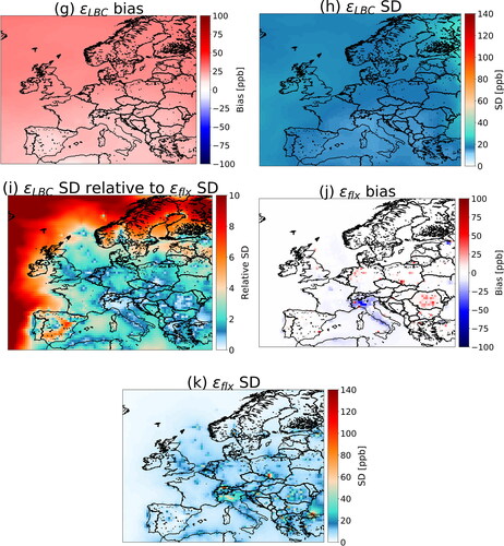
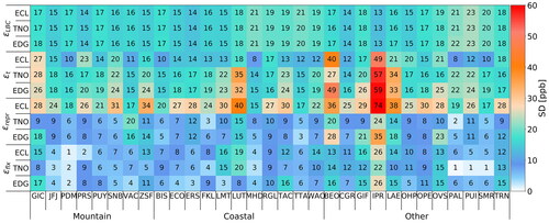
Fig. 7. Standard deviations (SDs) of
and
for 2015 at the 31 selected measurement sites (details in ). The colour and number give the same information.
Patterns due to the emissions show up both in and
The SD of
ranges between 1 and 80 ppb over land and reaches high values at several grid cells that contain emission hot-spots such as capitals in Europe, that is, Madrid, Paris and Warsaw. Maxima are found in high-emitting zones, such as the Silesian Coal Basin in Poland or the Po Valley in Italy (). A maximum value of 80 ppb occurs in St. Petersburg. Indeed, a hot-spot of emissions appears in St. Petersburg in the total emission map of the TNO-MACC_III inventory, due to fossil fuel related emissions (see ): 54% of the total GHG emissions in St. Petersburg come from energy sources (ISAP, 2019).
The SD of is in general much smaller over the sea than over the land, with values under 10 ppb, due to limited sea emissions. Nevertheless, higher values for the SD of
are found in the North Sea where numerous oil and gas off-shore platforms are located. The SD of
ranges between 10 and 140 ppb over land. High values are found over the largest emission hot-spots and areas () rather than in areas where the transport modelling is in principle more challenging, such as coasts or mountainous zones (high values for the Alps appear only in Italy and Switzerland). The patterns in
and
biases and SDs are linked to large gradients of concentrations induced by steep gradients of emissions, which have an impact even at a resolution as large as
Patterns due to meteorological situations and synoptic events may occasionally generate large errors but these events are averaged out at the yearly scale studied here.
Emission hot-spots and high-emitting zones are key regions of interest for policy makers. The capacity of retrieving information on the emissions through inversions in these areas would then be particularly useful. However, the very steep spatial emission gradients encountered at scales smaller than the smallest scale used in our work (0.25°) may lead to even higher and
than derived here. Hence, observations near hot-spots should be used with caution within an inversion over Europe at horizontal resolutions coarser than
The SD of ranges between 2 and 140 ppb and is the highest over grid cells where the emissions in the three inventories differ the most, for example, over the Po Valley, the Silesian Coal Basin, Istanbul (). Wunch et al. (Citation2019) have shown that there is an uncertainty in the spatial distribution of the emissions, based on the comparison of EDGAR v4.2 FT2010 (Olivier and Janssens-Maenhout, Citation2011) and TNO-MACC_III over parts of Europe, the differences being larger near large cities. Nevertheless,
is not necessarily the highest near large cities in our case because of the horizontal resolutions used in the simulations remain larger than the typical scale of European mega-cities.
4.2.2. Ratios of and relative to
The ratios of the SDs of
and
relative to the SD of
called hereafter
(, f, i), are used as indicators of whether
dominates the other types of error.
is the smallest relative error at about 1 over the entire domain ();
and
are often 2–6 () and therefore dominate
Even though information about the statistics of these errors makes it possible to characterise them correctly, the resulting observation error matrix may be too complex due to technical limitations, for example, it is too big for the system to deal with it in an affordable computing time. In this case, it is possible to include other variables, alongside the targeted emissions, in the control vector. In our case, the ratios of
and
relative to
indicate that
could be treated in the observation error statistics whereas the sources of
and
may better be controlled alongside the emissions in the inversion. Including LBCs in the control vector is usually done in regional inversions, but optimising the transport alongside emissions remains challenging in most state-of-the-art inversion systems, although first attempts exist (e.g. Zheng et al., Citation2018).
4.2.3. Temporal patterns in and
Annual biases appear in
and
(, a, d and j). As we have very few samples of errors (only three inventories), the average estimate is likely not representative of an actual bias, but rather indicates strong temporal correlations of errors.
and
auto-correlations have characteristic time scales generally less than 15 days ( and ), which correspond to the synoptic scale.
scales range mainly between 5 and 50 days and
scales are larger than one month over more than half the domain. In general, over continents,
and
have similar temporal scales. The similarity of structures requires that the magnitude of
is larger than the magnitudes of
and
to ensure efficient filtering by the inversion system.
Fig. 8. Characteristic time scales (in days) of the decrease of temporal auto-correlation for
and
over the domain for 2015.
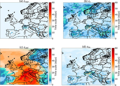
Fig. 9. Characteristic time scales (in days) of the decrease of temporal auto-correlation for
and
with the three inventories at the 31 selected measurement sites (details in ) for 2015.

4.2.4. Spatial correlations in and
The average spatial correlation structures of the different errors are presented in . The longest characteristic scale is found for (2450 km) and the shortest for
(100 km) and
(
50–100 km). The length of
is intermediate (
150–550 km). Lengths shorter than the size of one grid cell (
50 km) indicate that spatial correlations may be neglected, as is the case for
for EDGAR v4.3.2 and TNO-MACC_III. This suggests that a network of stations with a density higher than one station per 500 km would allow an inversion system to filter LBC and transport errors as their characteristic lengths are larger than 500 km with EDGAR v4.3.2 and TNO-MACC_III. However, our results show that distinguishing between representation and transported-emission errors is challenging without a very dense network (<100 km). Most of the sites used in this study are located at distances >100 km from each other, with only three groups of sites at <100 km: (i) IPR, PRS, JFJ, BEO and LAE in Switzerland and Northern Italy, (ii) GIF, OVS and TRN in France and (iii) TAC and WAO in the UK (see list of sites in ).
Fig. 10. Spatial correlations over the whole domain for the three estimates of
and
(indicated by the name of the emission inventory used, see Section 3.2 for details) and for the estimate of
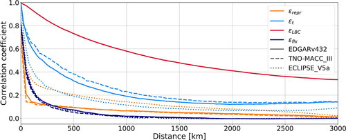
Most studies, such as Bergamaschi et al. (2018), Tsuruta et al. (2017), Locatelli et al. (2013) or Fortems-Cheiney et al. (Citation2012), assume the concentration errors to be spatially uncorrelated, which is not what we would recommend following our results. In our case, not taking into account correlations due to error patterns common to various measurement locations would artificially increase the weight of observations in the cost function used in the inversion and erroneously attribute all correlated patterns to the emissions. This implies that non-diagonal correlation matrices in observation states should be used for the inversion, for which smart implementations are required. This would be more crucial in inversions using satellite data, where the main source of correlation is the uncertainties in radiative transfer inversions to obtain total column CH4 observations. Furthermore, the spatial coverage of satellite data is more dense than data of uneven and sparse surface networks. Also, the same instrument is making the measurements. For these reasons, error correlations in space and/or time may occur and necessitate to account for off-diagonal terms in the observation variance–covariance matrix. This could be crucial, especially for instruments with a large swath and short revisit time, producing a lot of neighbouring data. Since satellite data are vertically integrated, the here presented errors may differ and should thus be recomputed when using satellite data for inversions.
4.2.5. Total concentration errors
The total concentration errors at the domain scale range between 14 and 422 ppb, with an average of 29 ppb, and between 21 and 53 ppb at the measurement site locations (see ). The total values per site category are similar with averages of 43 ppb, 40 ppb and 42 ppb for coastal, mountain and ‘other’ sites. The total concentration errors at the Swiss sites BEO, JFJ and LAE can be compared to the ones used in the study of Henne et al. (Citation2016). The total error for BEO and LAE (called LHW in Henne et al. Citation2016) with 38 and 46 ppb, respectively, compare well with the ranges of total errors of 1–41 ppb for BEO and 14–44 ppb for LAE in the different inversion set-ups in Henne et al. (Citation2016). For JFJ, our estimate of 46 ppb is higher than 14–20 ppb in their study. Ranges for combined measurement and model errors for CH4 are also reported in the study of Bergamaschi et al. (Citation2015). Our estimates are in the lower range of their set-ups with the LMDz-4DVAR (3–450 ppb) and TM5-4DVAR (3–1000 ppb) inversion systems and above the range of 10–30 ppb with TM3-STILT (except for GIC with 21 ppb).
Table 6. Total errors [ppb] in the concentration space at the location of measurement sites (see more information on sites and locations in and in ).
5. Conclusions and recommendations
This study aims at estimating errors that need to be taken into account in atmospheric inversions of CH4 emissions at the European scale. We have used a simple (i.e. technically ready and not expensive in computing time) and easy to update method that consists of performing a set of simulations using two limited-area CTMs at three different horizontal resolutions with inputs based on three anthropogenic emission inventories, three data sets of natural emissions and two sets of boundary and initial conditions. The analysis presented here can be applied for any atmospheric species and extended to any other region as long as the required components (sufficient number of emission inventories, multiple CTMs and LBC products) are available. For example, the USA or China would be a good option as the required components are available for them.
We have performed the analysis for the year 2015. Four types of errors have been estimated by computing differences of simulated hourly mixing ratios:
the background error
the representation error
the transport error
the transported-emission error
To be consistent with the usual choice of data based on expert knowledge, the errors have been computed from afternoon values (13–17 h UTC included) for non-mountain sites and from night-time values (00–04 h UTC included) for mountain sites, either in all the first-model-layer grid cells of the European domain or at the locations (horizontal and vertical grid cell) of 31 selected measurement sites. We have shown that this choice is not always optimal depending on stations and that it should be reassessed by inverse modellers (e.g. by using a method similar to the one described in Sections 3.4 and S3).
The methodology used in this study to estimate errors is specific to our set-up of CHIMERE (coarse horizontal resolution, chosen inputs) for continental scale CH4 emissions using a set of in situ monitoring sites. Nevertheless, the obtained error estimates allow us to gain insights into how these errors could be treated in a data assimilation system for inverting CH4 emissions at the European scale, as summarised in :
Table 7. Summary of the errors estimated in this study: main recommendations to treat each error in an inversion system for targeting CH4 emissions in Europe at the yearly scale and orders of magnitude of correlation lengths which can be used to simply represent some of them.
The spatial correlation lengths estimated here show that some error patterns cover a number of measurement sites, whereas errors in in situ fixed measurements are generally assumed to be uncorrelated in inversion systems.
Moreover, we have estimated the error in the emission inventories, particularly at the country and sector (agriculture, waste, fossil fuel related emissions and wetlands) scales as atmospheric inversions require prior emission errors in their statistics of the emission space. Due to the assumptions and proxies used for the spatial distribution of area and point sources in the inventories, they differ the most for the waste and fossil fuel related sectors and agree better for agriculture at the European scale. The disagreements are particularly due to some high-emitting zones or hot-spots not being represented consistently, that is, their locations and/or emissions vary between the three inventories. Discrepancies also arise from the projection of emissions onto the model’s grid along the coasts, which may impact specifically the assimilation of data from coastal measurement sites. All cases where emission gradients between two neighbouring types of land-use are steep will lead to such an issue. Spatial correlation lengths that are recommended to represent
for agricultural emissions are
100–150 km. Cross-sector and cross-sector cross-country correlations show the impact of spatial correlations that are used in the inventories. Our simple analysis based on the available inventories indicates that errors are heterogeneous and depend on the sector and country, which is in contrast with most inversion studies where the assumed uncertainties are homogeneous, with only land being different from sea. Finally, there is a need for an in-depth analysis and/or update of the spatial distribution of current emission inventories and for a more complete error estimation study dedicated to emission inventories.
Following the method chosen here, further work should target the following:
Acknowledgements
We are grateful to the colleagues at TNO for their valuable support. We thank Matthew Lang, Diego Santaren and Audrey Fortems-Cheiney for their helpful advice. Calculations were performed using the resources of LSCE, maintained by François Marabelle and the LSCE IT team. We thank the PIs of the measurement sites we used in this study for maintaining methane measurements and for sharing their data through the following contributors: World Data Centre for Greenhouse Gases (WDCGG), Institut Català de Ciències del Clima (IC3), Swiss Federal Laboratories for Materials Science and Technology (Empa), Laboratoire des Sciences du Climat et de lEnvironnement (LSCE), Ricerca sul Sistema Energetico (RSE), Integrated non-CO2 Greenhouse gas Observing System (InGOS), Integrated Carbon Observation System (ICOS), Umweltbundesamt (UBA), Environmental Chemical Process Laboratory (ECPL), National Oceanic and Atmospheric Administration (NOAA) Earth System Research Laboratories (ESRL), University of Bristol, Norwegian Institute for Air Research (NILU), University of Bern, Joint Research Centre (JRC), Observatoire des Sciences de lUnivers Institut Pythéas (OSU), Finnish Meteorological Institute (FMI), and University of Helsinki.
Disclosure statement
The authors declare no competing interests.
Data availability statement
The data that support the findings of this study are available from the corresponding author upon request.
Supplemental data
Supplemental data for this article can be accessed here.
Additional information
Funding
References
- Arora, V. K., Melton, J. R. and Plummer, D. 2018. An assessment of natural methane fluxes simulated by the CLASS-CTEM model. Biogeosciences 15, 4683–4709. https://bg.copernicus.org/articles/15/4683/2018/.
- Berchet, A., Pison, I., Chevallier, F., Bousquet, P., Bonne, J.-L. and co-authors. 2015. Objectified quantification of uncertainties in Bayesian atmospheric inversions. Geosci. Model Dev. 8, 1525–1546. https://www.geosci-model-dev.net/8/1525/2015/.
- Bergamaschi, P., Corazza, M., Karstens, U., Athanassiadou, M., Thompson, R. and co-authors. 2015. Top-down estimates of European CH4 and N2O emissions based on four different inverse models. Atmos. Chem. Phys. 15, 715–736. doi:https://doi.org/10.5194/acp-15-715-2015
- Bergamaschi, P., Karstens, U., Manning, A. J., Saunois, M., Tsuruta, A. and co-authors. 2018. Inverse modelling of European CH4 emissions during 2006–2012 using different inverse models and reassessed atmospheric observations. Atmos. Chem. Phys. 18, 901–920. https://www.atmos-chem-phys.net/18/901/2018/.
- Bergamaschi, P., Krol, M., Dentener, F., Vermeulen, A., Meinhardt, F. and co-authors. 2005. Inverse modelling of national and European CH4 emissions using the atmospheric zoom model TM5. Atmos. Chem. Phys. 5, 2431–2460. https://www.atmos-chem-phys.net/5/2431/2005/.
- Bergamaschi, P., Krol, M., Meirink, J. F., Dentener, F., Segers, A. and co-authors. 2010. Inverse modeling of European CH4 emissions 2001–2006. J. Geophys. Res.: Atmos. 115, D22309. https://agupubs.onlinelibrary.wiley.com/doi/abs/10.1029/2010JD014180.
- Bocquet, M., Wu, L., and Chevallier, F. 2011. Bayesian design of control space for optimal assimilation of observations. Part I: Consistent multiscale formalism. Q. J. R Meteorolog. Soc. 137, 1340–1356. https://rmets.onlinelibrary.wiley.com/doi/abs/10.1002/qj.837.
- Bousquet, P., Ciais, P., Miller, J. B., Dlugokencky, E. J., Hauglustaine, D. A. and co-authors. 2006. Contribution of anthropogenic and natural sources to atmospheric methane variability. Nature 443, 439–443. doi:https://doi.org/10.1038/nature05132
- Bousquet, P., Pierangelo, C., Bacour, C., Marshall, J., Peylin, P. and co-authors. 2018. Error budget of the methane remote Lidar mission and its impact on the uncertainties of the global methane budget. Journal of Geophysical Research: Atmospheres 123, 11,766–11,785. https://agupubs.onlinelibrary.wiley.com/doi/abs/10.1029/2018JD028907.
- Bousquet, P., Ringeval, B., Pison, I., Dlugokencky, E. J., Brunke, E.-G. and co-authors. 2011. Source attribution of the changes in atmospheric methane for 2006–2008. Atmos. Chem. Phys. 11, 3689–3700. https://www.atmos-chem-phys.net/11/3689/2011/.
- Broquet, G., Chevallier, F., Rayner, P., Aulagnier, C., Pison, I. and co-authors. 2011. A European summertime CO2 biogenic flux inversion at mesoscale from continuous in situ mixing ratio measurements. J. Geophys. Res.: Atmos. 116, D23303. https://agupubs.onlinelibrary.wiley.com/doi/abs/10.1029/2011JD016202.
- Dabberdt, W., Carroll, M., Baumgardner, D., Carmichael, G., Cohen, R. and co-authors. 2004. Meteorological research needs for improved air quality forecasting: report of the 11th prospectus development team of the U.S. Weather Research Program. Bull. Amer. Meterol. Soc. 85, 563. doi:https://doi.org/10.1175/BAMS-85-4-563
- EEA. 2019. Annual European Union greenhouse gas inventory 1990–2017 and inventory report 2019. https://www.eea.europa.eu/publications/european-union-greenhouse-gas-inventory-2019.
- Fortems-Cheiney, A., Chevallier, F., Pison, I., Bousquet, P., Saunois, M. and co-authors. 2012. The formaldehyde budget as seen by a global-scale multi-constraint and multi-species inversion system. Atmos. Chem. Phys. 12, 6699–6721. https://www.atmos-chem-phys.net/12/6699/2012/.
- Fortems-Cheiney, A., Pison, I., Dufour, G., Broquet, G., Berchet, A. and co-authors. 2019. Variational regional inverse modeling of reactive species emissions with PYVAR-CHIMERE. Geosci. Model Dev. Discuss. 2019, 1–22. https://www.geosci-model-dev-discuss.net/gmd-2019-186/.
- Ganesan, A. L., Rigby, M., Zammit-Mangion, A., Manning, A. J., Prinn, R. G. and co-authors. 2014. Characterization of uncertainties in atmospheric trace gas inversions using hierarchical Bayesian methods. Atmos. Chem. Phys. 14, 3855–3864. https://www.atmos-chem-phys.net/14/3855/2014/.
- Hayman, G. D., O’Connor, F. M., Dalvi, M., Clark, D. B., Gedney, N. and co-authors. 2014. Comparison of the HadGEM2 climate–chemistry model against in situ and SCIAMACHY atmospheric methane data. Atmos. Chem. Phys. 14, 13257–13280. https://acp.copernicus.org/articles/14/13257/2014/.
- Henne, S., Brunner, D., Oney, B., Leuenberger, M., Eugster, W. and co-authors. 2016. Validation of the Swiss methane emission inventory by atmospheric observations and inverse modelling. Atmos. Chem. Phys. 16, 3683–3710. https://www.atmos-chem-phys.net/16/3683/2016/.
- Hourdin, F., Musat, I., Bony, S., Braconnot, P., Codron, F. and co-authors. 2006. The LMDZ4 general circulation model: climate performance and sensitivity to parametrized physics with emphasis on tropical convection. Clim. Dyn. 27, 787–813. doi:https://doi.org/10.1007/s00382-006-0158-0
- Hu, H., Landgraf, J., Detmers, R., Borsdorff, T., Aan de Brugh, J. and co-authors. 2018. Toward global mapping of methane with TROPOMI: first results and intersatellite comparison to GOSAT. Geophys. Res. Lett. 45, 3682–3689. https://agupubs.onlinelibrary.wiley.com/doi/abs/10.1002/2018GL077259.
- IPCC. 2013. Summary for policymakers. In: Climate Change 2013: The Physical Science Basis. Contribution of Working Group I to the Fifth Assessment Report of the Intergovernmental Panel on Climate Change (ed. T. F. Stocker, D. Qin, G.-K. Plattner, M. Tignor, S. K. Allen, J. Boschung, A. Nauels, Y. Xia, V. Bex and P. M. Midgley), Cambridge, United Kingdom and New York, NY, USA. Cambridge University Press, pp. 1–30. www.climatechange2013.org.
- IPCC. 2006. IPCC Guidelines for National Greenhouse Gas Inventories, Prepared by the National Greenhouse Gas Inventories Programme (ed. H. S. Eggleston, L. Buendia, K. Miwa, T. Ngara and K. Tanabe). Institute for Global Environmental Strategies, Japan.
- ISAP. 2019. Integrated Sustainability Action Plan. http://www.stpete.org/sustainability/integrated_sustainability_action_plan.php.
- Janssens-Maenhout, G., Crippa, M., Guizzardi, D., Muntean, M., Schaaf, E. and co-authors. 2019. EDGAR v4.3.2 Global Atlas of the three major greenhouse gas emissions for the period 1970–2012. Earth Syst. Sci. Data 11, 959–1002. https://essd.copernicus.org/articles/11/959/2019/.
- Jonas, M., Marland, G., Winiwarter, W., White, T., Nahorski, Z. and co-authors. 2011. Benefits of dealing with uncertainty in greenhouse gas inventories: introduction. In: Greenhouse Gas Inventories: Dealing with Uncertainty, Springer Netherlands, Dordrecht, pp. 3–18. https://doi.org/https://doi.org/10.1007/978-94-007-1670-4_2.
- Kaminski, T., Rayner, P., Heimann, M., and and Enting, I. 2001. On aggregation errors in atmospheric transport inversion. J. Geophys. Res. 106, 4703–4715. doi:https://doi.org/10.1029/2000JD900581
- Koffi, E., Bergamaschi, P., Karstens, U., Krol, M., Segers, A. J. and co-authors. 2016. Evaluation of the boundary layer dynamics of the TM5 model. Geosci. Model Dev. Discuss. 9, 1–37.
- Kuenen, J. J. P., Visschedijk, A. J. H., Jozwicka, M. and Denier van der Gon, H. A. C. 2014. TNO-MACC_II emission inventory; a multi-year (2003–2009) consistent high-resolution European emission inventory for air quality modelling. Atmos. Chem. Phys. 14, 10963–10976. https://www.atmos-chem-phys.net/14/10963/2014/.
- Locatelli, R., Bousquet, P., Chevallier, F., Fortems-Cheney, A., Szopa, S. and co-authors. 2013. Impact of transport model errors on the global and regional methane emissions estimated by inverse modelling. Atmos. Chem. Phys. 13, 9917–9937. https://www.atmos-chem-phys.net/13/9917/2013/.
- Locatelli, R., Bousquet, P., Hourdin, F., Saunois, M., Cozic, A. and co-authors. 2015. Atmospheric transport and chemistry of trace gases in LMDz5B: evaluation and implications for inverse modelling. Geosci. Model Dev. 8, 129–150. https://gmd.copernicus.org/articles/8/129/2015/.
- Lunt, M. F., Rigby, M., Ganesan, A. L. and Manning, A. J. 2016. Estimation of trace gas fluxes with objectively determined basis functions using reversible-jump Markov chain Monte Carlo. Geosci. Model Dev. 9, 3213–3229. https://www.geosci-model-dev.net/9/3213/2016/.
- Mailler, S., Menut, L., Khvorostyanov, D., Valari, M., Couvidat, F. and co-authors. 2017. CHIMERE-2017: from urban to hemispheric chemistry–transport modeling. Geosci. Model Dev. 10, 2397–2423. https://www.geosci-model-dev.net/10/2397/2017/.
- Manders, A., Builtjes, P. J. H., Curier, L., Denier van der Gon, H., Hendriks, C. and co-authors. 2017. Curriculum vitae of the LOTOS-EUROS (v2.0) chemistry transport model. Geosci. Model Dev. Discuss. 10, 1–53.
- Manning, A. J., Doherty, S., O’ Jones, A. R., Simmonds, P. G. and Derwent, R. G. 2011. Estimating UK methane and nitrous oxide emissions from 1990 to 2007 using an inversion modeling approach. J. Geophys. Res.: Atmos. 116, D02305. https://agupubs.onlinelibrary.wiley.com/doi/abs/10.1029/2010JD014763.
- Marécal, V., Peuch, V.-H., Andersson, C., Andersson, S., Arteta, J. and co-authors. 2015. A regional air quality forecasting system over Europe: the MACC-II daily ensemble production. Geosci. Model Dev. 8, 2777–2813. https://www.geosci-model-dev.net/8/2777/2015/.
- McNorton, J., Bousserez, N., Agustí-Panareda, A., Balsamo, G., Choulga, M. and co-authors. 2020. Representing model uncertainty for global atmospheric CO2 flux inversions using ECMWF-IFS-46R1. Geosci. Model Dev. Discuss. 2020, 1–30. https://www.geosci-model-dev-discuss.net/gmd-2019-314/.
- Menut, L., Bessagnet, B., Khvorostyanov, D., Beekmann, M., Blond, N. and co-authors. 2013. CHIMERE 2013: a model for regional atmospheric composition modelling. Geosci. Model Dev. 6, 981–1028. https://www.geosci-model-dev.net/6/981/2013/.
- National Academies of Sciences, Engineering, and Medicine. 2018. Improving Characterization of Anthropogenic Methane Emissions in the United States, 4 Addressing Uncertainties in Anthropogenic Methane Emissions. The National Academies Press, Washington, DC. https://www.ncbi.nlm.nih.gov/books/NBK519298/.
- Olivier, J. and Janssens-Maenhout, G. 2011. Part III: greenhouse gas emissions. In: CO2 emissions from fuel combustion. Paris (France): International Energy Agency (IEA). https://publications.jrc.ec.europa.eu/repository/handle/JRC67519.
- Peltola, O., Vesala, T., Gao, Y., Räty, O., Alekseychik, P. and co-authors. 2019. Monthly gridded data product of northern wetland methane emissions based on upscaling eddy covariance observations. Earth Syst. Sci. Data 11, 1263–1289. https://www.earth-syst-sci-data.net/11/1263/2019/.
- Pison, I., Berchet, A., Saunois, M., Bousquet, P., Broquet, G. and co-authors. 2018. How a European network may help with estimating methane emissions on the French national scale. Atmos. Chem. Phys. 18, 3779–3798. https://www.atmos-chem-phys.net/18/3779/2018/.
- Ringeval, B., de Noblet-Ducoudré, N., Ciais, P., Bousquet, P., Prigent, C. and co-authors. 2010. An attempt to quantify the impact of changes in wetland extent on methane emissions on the seasonal and interannual time scales. Global Biogeochem. Cycles 24, GB2003. https://agupubs.onlinelibrary.wiley.com/doi/abs/10.1029/2008GB003354.
- Ringeval, B., Friedlingstein, P., Koven, C., Ciais, P., de Noblet, N. and co-authors. 2011. Climate-CH4 feedback from wetlands and its interaction with the climate-CO2 feedback. Biogeosciences 8, 2137–2157. doi:https://doi.org/10.5194/bg-8-2137-2011
- Saunois, M., Bousquet, P., Poulter, B., Peregon, A., Ciais, P. and co-authors. 2016a. The global methane budget 2000–2012. Earth Syst. Sci. Data 8, 697–751. https://www.earth-syst-sci-data.net/8/697/2016/.
- Saunois, M., Jackson, R. B., Bousquet, P., Poulter, B. and Canadell, J. G. 2016b. The growing role of methane in anthropogenic climate change. Environ. Res. Lett. 11, 120207. doi:https://doi.org/10.1088/1748-9326/11/12/120207
- Segers, A. and Houweling, S. Description of the CH4 Inversion Production Chain. ECMWF Copernicus Report, 2017. URL https://atmosphere.copernicus.eu/sites/default/files/2020-01/CAMS73_2018SC1_D73.5.2.2-2019_202001_production_chain_v1.pdf.
- Stohl, A., Aamaas, B., Amann, M., Baker, L. H., Bellouin, N. and co-authors. 2015. Evaluating the climate and air quality impacts of short-lived pollutants. Atmos. Chem. Phys. 15, 10529–10566. https://www.atmos-chem-phys.net/15/10529/2015/.
- Tarantola, A. 2005. Inverse Problem Theory and Methods for Model Parameter Estimation. Society for Industrial and Applied Mathematics, Philadelphia, PA.
- Thompson, R. L., Sasakawa, M., Machida, T., Aalto, T., Worthy, D. and co-authors. 2017. Methane fluxes in the high northern latitudes for 2005–2013 estimated using a Bayesian atmospheric inversion. Atmos. Chem. Phys. 17, 3553–3572. https://www.atmos-chem-phys.net/17/3553/2017/.
- Thompson, R. L., Stohl, A., Zhou, L. X., Dlugokencky, E., Fukuyama, Y. and co-authors. 2015. Methane emissions in East Asia for 2000–2011 estimated using an atmospheric Bayesian inversion. J. Geophys. Res.: Atmos. 120, 4352–4369. https://agupubs.onlinelibrary.wiley.com/doi/abs/10.1002/2014JD022394.
- Tsuruta, A., Aalto, T., Backman, L., Hakkarainen, J., van der Laan-Luijkx, I. T. and co-authors. 2017. Global methane emission estimates for 2000–2012 from CarbonTracker Europe-CH4 v1.0. Geosci. Model Dev. 10, 1261–1289. https://www.geosci-model-dev.net/10/1261/2017/.
- Tsuruta, A., Aalto, T., Backman, L., Krol, M. C., Peters, W. and co-authors. 2019. Methane budget estimates in Finland from the CarbonTracker Europe-CH4 data assimilation system. Tellus B: Chem. Phys. Meteorol. 71, 1–20. https://doi.org/https://doi.org/10.1080/16000889.2018.1565030.
- Varon, D. J., McKeever, J., Jervis, D., Maasakkers, J. D., Pandey, S. and co-authors. 2019. Satellite discovery of anomalously large methane point sources from oil/gas production. Geophys. Res. Lett. 46, 13507–13516. https://agupubs.onlinelibrary.wiley.com/doi/abs/10.1029/2019GL083798.
- Wang, F., Maksyutov, S., Tsuruta, A., Janardanan, R., Ito, A. and co-authors. 2019. Methane emission estimates by the global high-resolution inverse model using national inventories. Remote Sensing 11, 2489. https://www.mdpi.com/2072-4292/11/21/2489.
- Wang, Y., Broquet, G., Ciais, P., Chevallier, F., Vogel, F. and co-authors. 2017. Estimation of observation errors for large-scale atmospheric inversion of CO2 emissions from fossil fuel combustion. Tellus B: Chem. Phys. Meteorol. 69, 1325723. doi:https://doi.org/10.1080/16000889.2017.1325723
- Wunch, D., Jones, D. B. A., Toon, G. C., Deutscher, N. M., Hase, F. and co-authors. 2019. Emissions of methane in Europe inferred by total column measurements. Atmos. Chem. Phys. 19, 3963–3980. https://www.atmos-chem-phys.net/19/3963/2019/. doi:https://doi.org/10.5194/acp-19-3963-2019
- Zheng, T., French, N. H. F., and and Baxter, M. 2018. Development of the WRF-CO2 4D-Var assimilation system v1.0. Geosci. Model Dev. 11, 1725–1752. https://gmd.copernicus.org/articles/11/1725/2018/.