Confounding in longitudinal studies in addiction treatment research

Abstract

Background: The effectiveness of treatment for people with substance use disorders is usually examined using longitudinal cohorts. In these studies, treatment is often considered as a time-varying exposure. The aim of this commentary is to examine confounding in this context, when the confounding variable is time-invariant and when it is time-varying.

Method: Types of confounding are described with examples and illustrated using path diagrams. Simulations are used to demonstrate the direction of confounding bias and the extent that it is accounted for using standard regression adjustment techniques.

Results: When the confounding variable is time invariant or time varying and not influenced by prior treatment, then standard adjustment techniques are adequate to control for confounding bias, provided that in the latter scenario the time-varying form of the variable is used. When the confounder is time varying and affected by prior treatment status (i.e. it is a mediator of treatment), then standard methods of adjustment result in inconsistency.

Conclusions: In longitudinal cohorts where treatment exposure is time varying, confounding is an issue which should be considered, even if treatment exposure is initially randomized. In these studies, standard methods of adjustment may result be inadequate, even when all confounders have been identified. This occurs when the confounder is also a mediator of treatment. This is a likely scenario in many studies in addiction.

Keywords:

• Addiction research
• longitudinal studies
• time-varying confounding
• cohort studies

Introduction

A treatment provided to people with substance-use disorder is judged effectively by the extent that it changes a person’s behavior, over and above what would have occurred without treatment (Prochaska et al. 1992). In order to quantify change attributable to treatment, many studies use cohorts of substance users, longitudinally followed-up, comparing an outcome between those exposed to treatment and those not. A major consideration when estimating the effect of treatment is whether the contrast between exposed and unexposed groups is unbiased or whether it is subject to confounding, which occurs when treatment exposure and outcome share a common cause (Hernán & Robins 2016). In situations when confounding is present, a crude (unadjusted) comparison between exposed and unexposed will, at least in part, reflect the dual influence that the confounding variable has and will therefore be biased. The standard approach for adjusting for confounding is to condition the contrast between exposed and unexposed on levels of the confounder, for example by including them as covariates in a regression model.

In many studies in substance use research, the effectiveness of treatment is quantified by contrasting an outcome between periods when subjects are being treated with periods when they are not. For example, the extent that opiate substitution therapy reduces offending has often been investigated by comparing the offending rate during periods in OST to that seen during periods out (Bukten et al. 2012; Campbell et al. 2007; Larney et al. 2012; Lind et al. 2005). People with substance use disorders often cycle in and out of treatment (Dennis et al. 2005); therefore, treatment exposure is unlikely to remain stationary and is characterized by a time-varying variable. If there are non-random factors which influence whether subjects are in treatment and these are also related to the outcome, then this contrast is subject to confounding. When treatment exposure is time varying, then it will often be necessary to account for time-varying confounders.

The current paper discusses confounding biases which may arise in longitudinal substance use research when treatment exposure is time varying. It begins by considering the case of a single time-invariant confounding variable; then examines the case of a time-varying confounding variable; and finishes by considering the case of a time-varying confounding variable that is affected by prior treatment status. In this latter case, the confounder is referred to as a mediator of treatment effect. In this situation standard methods of adjustment, such as adjustment in a regression model, can no longer be used to account for the confounding without resulting in inconsistency or bias. We introduce an alternative to regression adjustment – the Inverse Probability of Treatment Weight method – that provides unbiased estimates in the presence of a time-varying confounder. In the following sections, confounding scenarios are illustrated through examples from substance use research, path diagrams and simulations.

Confounding by a time-invariant variable

When contrasting an outcome between treated and untreated periods, if there is a factor which has a dual influence on whether a subject is in treatment at any given time and whether the outcome occurs at that time, then the measure of treatment effectiveness will be biased due to confounding. The simplest case of confounding in this situation exists when the confounding variable remains constant (time-invariant) over follow-up. The path diagram in Figure 1(a) illustrates the case, where being treated (A) and outcome (Y) is measured longitudinally over follow-up (t = 1 ⋯ T) and there is a time-invariant variable (X) which has an effect on both treatment and outcome. An unadjusted analysis in this situation would measure an association between treatment and outcome, even if treatment had no effect. This biased path is illustrated with a red line. For example, in a study looking at the effect of treatment on offending risk among opioid users, if gender is related to treatment retention and offending risk, then an analysis which does not account for gender will be biased.

Figure 1. Path diagrams representing a time varying treatment exposure (A_t), an outcome variable (Y_t) and confounding by a variable (X) that is (a) time invariant; (b) time-varying and not affected by prior treatment; and (c) time-varying and affected by prior treatment.

This confounding was demonstrated with a simulation. Here, 200 subjects were simulated to represent daily records covering 2 years, from t = 0 to 730. The probability of whether a subject (i) was in treatment (A) on given day (t) was a function of a time-invariant variable (X) and strongly influenced by the treatment status on the day prior (A_t - 1):

The probability of an outcome event occurring on a day was also simulated as a function of the same time-invariant variable and a weak correlation with whether an event occurred on the previous day:

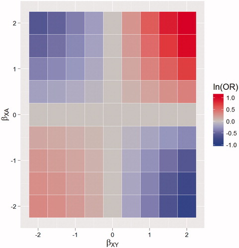
These probabilities were inputs for a random Bernoilli process, used to simulate whether, on a given day, a subject had an outcome event and was in treatment. The X_i’s correspond to a binary variable which was randomly present in 25% of subjects and which has an effect (on the log scale) of changing the odds of being in treatment on a day by β_XA. For example, A could be an indicator for whether the ith subject was in opioid substitution therapy on day t, X_i could be a binary indicator for female gender and Y indicates whether a crime was recorded on the same day. For this simulation, β_XA and β_XY were varied between −2 and 2, in increments of 0.1 representing different confounding effects. A logistic regression model for treatment on outcome was fitted to each simulation, ignoring the confounding variable. In order to reduce the error of the estimates, 1000 Monte Carlo simulations were created for each combination of β_XA and β_XY and the log odds ratios were averaged across datasets. Because there was no simulated effect of treatment on outcome, any significant diversion from 0 indicates bias.

The resulting bias associated with the treatment variable is shown in Figure 2. This shows clearly that if a variable is dually associated with the likelihood of being in treatment and outcome at the same time then an unadjusted analysis will be biased. The presence of such a confounder is likely in many instances. For example, female opioid users have been found to have longer episodes of treatment (National Treatment Agency for Substance misuse 2010) and to have a lower rate of offending (Pierce et al. 2015). Therefore, studies which investigate the effect of treatment on offending but fail to adjust for gender in their analysis, will underestimate the true effect of treatment.

Figure 2. Time-invariant confounding: heat maps of the bias of the estimated treatment effect, on the log odds ratio (ln(OR)) scale, when failing to control for confounding. With varying effect of a confounding variable on being in treatment (β_XA) and outcome (β_XY). The area in blue represents negative bias, the area in red positive bias.

Confounding by a time-varying variable

Many variables change with passing time and if those variables affect the likelihood of an outcome and treatment exposure then they are classed as time-varying confounders. This situation is illustrated in the path diagram in Figure 1(b) with the biased path again shown by a red line. In order to properly account for the bias introduced by time-varying confounders, a time-varying variable is needed in the analysis: controlling for a time-invariant form of the variable will only control for part of the confounding effect. For example, in a study of morbidity and treatment among alcoholics, a person’s age might be considered as a confounder. The effect that age has on treatment retention and outcome is related to their age at that particular time, not its value at a fixed prior time. Therefore, it is not sufficient to use ‘age at baseline’ to adjust for the confounding effect of age.

A further simulation was run to demonstrate time-varying confounding and the bias which remains after adjustment using a time-invariant version. The data were generated using the same specifications as previously, except that the confounding variable now varies and is indexed by its value at a given time (i.e. X_i becomes X_it). This variable was simulated to represent an age variable centered around its mean, using a normal distribution with mean zero and a standard deviation of one, and was scaled by 365 (i.e. increases by a unit each year).

Two logistic regression models were used to analyze these simulated data: an unadjusted model that completely omits the confounder X; and one which includes the value of the confounder when t = 0 (i.e. the baseline value). The resulting bias in the parameter associated with treatment exposure, for different effects of the confounder on outcome and treatment, is shown in Figure 3(a) and (b).

Figure 3. Time-varying confounding: Heat maps of the bias on the log odds ratio (ln(OR)) scale, when (a) there is no adjustment, (b) adjusting for the baseline value of the confounder only. With varying effect of a time-varying, deterministic, confounding variable on being in treatment (β_XA) and outcome (β_XY). The area in blue represents negative bias, the area in red positive bias.

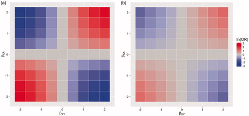
Figure 3(a) illustrates the bias in an unadjusted analysis when a time-varying variable has a dual effect on treatment exposure and outcome. Figure 3(b) demonstrates that only part of this bias is removed when the baseline value of the confounder is used for adjustment. Studies should, therefore, always use a time-varying version. For example, in a study of the effects of attending alcohol treatment on the risk of hospitalization, older alcohol users tend to have longer episodes of treatment (Mertens & Weisner 2000) and age also increases the likelihood of many morbidity outcomes (Rehm et al. 2003); therefore, age biases the comparison between treated and untreated periods. However, in order to properly account for the confounding effects of age in this scenario, a time-varying version of age must be used.

Age is classed as a deterministic time-varying variable because its value is solely determined by the passage of time. There may also be time-dependent, non-deterministic confounders. For example, in a study comparing the incidence of breathing difficulties for ex-smokers between periods when they are engaged with cognitive behavioral therapy and periods when they are not, a person’s level of stress is a likely confounder because it increases a person’s risk of smoking relapse (Cohen & Lichtenstein 1990) and their likelihood of breathing difficulties (Smoller et al. 1996). A person’s level of stress will likely fluctuate over any period, due to a range of non-deterministic factors such as sleep (Dusselier et al. 2005) or exercise (Salmon, 2001). As the next section demonstrates, the existence of non-deterministic, time-varying confounders require further attention, because if the variable is also influenced by prior treatment exposure, then standard methods of adjustment will fail.

Time-varying confounder affected by prior treatment status

In many substance-use disorder cohorts, there will be non-deterministic, time-varying variables with the dual role of a confounder that are also targeted by the treatment under consideration. For example, in an analysis of the effect of opiate substitution therapy on mortality, injecting, as a route of drug administration, increases mortality risk (Pierce et al. 2015) and is also negatively associated with treatment retention (Magura et al. 1998) and so qualifies as a confounder. Also, opiate substitution therapy reduces the risk of injecting (Simpson et al. 1997). This situation is illustrated in the path diagram in Figure 1(c). Because injecting is a confounder, it will bias the relationship between treatment and outcome (shown by a red line in Figure 1(c)).

Here, because prior treatment reduces injecting risk and that in turn reduces the risk of the outcome, the variable acts as a mediator of treatment on outcome. The change in a mediator describes a mechanism through which treatment achieves a change in outcome and it is (at least partly) through this change that treatment is effective. For any causal effect from treatment to outcome, there will be many mediators; however, only a subset will also be confounders. The mediating mechanism is illustrated by the green arrows in Figure 1(c).

In the presence of a mediator, the effect of treatment can be split between the indirect effect, which is the effect on outcome that comes about from changes in the mediated variable, and the direct effect, which is the effect of treatment that is not through changes in the mediator. We are usually interested in the combination of the indirect and the mediated effect, referred to as the total effect of treatment. Including a mediator variable in an adjusted regression model of treatment on outcome will yield the treatment’s direct effect. Estimation of the indirect effect is not covered in this paper, but can be obtained (under strong modeling assumptions) by contrasting the total and the direct effects (Baron & Kenny 1986). In the injecting example, regressing treatment on mortality, while controlling for injecting, will yield the direct effect of treatment, while not including injecting in the model will yield the total effect of treatment, albeit one that is biased due to confounding. Injecting, therefore, has the dual role of being a confounder and mediator. Using standard confounding adjustment techniques, there is a dilemma for the analysis team: either adjust for the variable to remove confounding bias, which will also remove the indirect effect that treatment has on the outcome; or do not control for the variable and have bias by confounding in the total effect.

One method that provides unbiased estimates of the total treatment effect in the presence of time-varying confounding is the Inverse Probability of Treatment Weighted (IPTW) approach (Robins et al. 2000). Here we provide a non-technical description of the IPTW approach. A more detailed description is available in the Supplementary material, as well as the Stata code for carrying out an analysis using this method.

The IPTW method estimates a marginal structural model – a model for each subjects’ potential outcome for a given treatment history. The outcomes are “potential” because they represent what a subject’s outcome value would be under all potential treatment histories, not just what was observed. The first step in the IPTW approach is to calculate the probability of being treated at each time-point, conditional on treatment and covariate history. This is the extension of the propensity score to the context of time-varying treatment. The next step reweights the cohort by the inverse of this predicted probability of treatment. Provided all confounders are identified, and the IPTW’s properly balance the groups, the reweighted sample represents a pseudo-population where treatment assignment is unconfounded at each time-point, analogous to a randomized trial. Analysis of the reweighted sample will, therefore, provide an unbiased estimation of the effect of treatment exposure on the (potential) outcome.

The issues described in this section are illustrated using a further simulation. Here the simulation is run as before, except now the value of a binary confounder (X) at time t is related to the value of treatment on the previous day (A_t - 1).):

The X_it variable could represent a behavioral variable that is a confounder and is affected by prior treatment status, for example injecting status. Two logistic regression models were fitted to the simulated data: an unadjusted model which included the treatment variable only and another model that adjusts for the time-varying confounder. Additionally the IPTW approach was used to calculate the “true” treatment effect of treatment. Bias in the unadjusted and the adjusted regression models was estimated by taking the difference between the log odds ratio associated with treatment from the regression approaches with that obtained from the IPTW approach.

The bias from three scenarios representing different strengths of the variable X on treatment β_XA and the outcome β_XA and different strengths of treatment on the confounder β_AX are shown in Table 1.

Table 1. Bias on the log odds ratio (ln(OR)) scale from simulations for different effects of a time-varying variable on treatment (β_XA) and outcome (β_XY) and the effect of prior treatment on that variable (β_AXAXE); unadjusted analysis and after adjusting for the time-varying variable.

				ln(OR) bias^a
Scenario	βXA	βXY	βAX	Unadjusted analysis	Adjusted analysis
1. X is a confounder and mediator	−2	2	2	−0.61	−0.14
2. X is a confounder only	−2	2	0	−0.72	0.02
3. X is a mediator only	0	2	2	0.00	−0.40

^a Bias calculated as the difference between regression estimates and estimates using the IPTW method, full details provided in Appendix A.

The first scenario is the one described above: the variable X is both a confounder and a mediator. In this case, both the unadjusted and the adjusted analyses yield biased results and so neither are appropriate. Scenario 2 shows that when X is a confounder only, the unadjusted analysis is biased, whereas the adjusted one is not. Conversely, when X is a mediator only, and not predictive of treatment (scenario 3), the adjusted analysis is unbiased whereas the unadjusted one is not.

Discussion

This paper provides an overview of confounding in longitudinal substance use disorder research with a time-varying treatment exposure. It considers scenarios where the confounder is both time-invariant and time varying. When confounding variables are time-invariant, or when the time-varying confounder is independent of prior treatment status, then standard regression adjustment methods will provide unbiased estimates, assuming all confounders are identified and properly adjusted for. When the confounding variable is both time varying and affected by prior treatment, it is not sufficient for all such confounders to be identified: regression adjustment will result in inconsistency. This arises because the confounding variable acts as a mediator of the effect of treatment, as well as a confounder, therefore, adjusting for it will remove the effect that treatment has on outcome through changes in this variable. This issue was first highlighted in occupational epidemiology (Robins 1986) and should be considered in any situation where both exposure and confounder are time varying.

We demonstrate the IPTW estimate of a marginal structural model as a solution for providing unbiased estimation of the treatment effect in the presence of time-varying confounding, when the confounder is affected by prior treatment status. There are a number of other analytical methods developed for unbiased estimation in this scenario. These include the g-computation formula (Robins 1986) and g-estimation (Robins et al. 1992). These have been implemented in many statistical software packages and extensively reviewed elsewhere, with full technical details (Daniel et al. 2013; Fewell et al. 2004; Robins et al. 2000).

The IPTW approach is the most commonly used in substance use disorder research to correct for time-varying confounding (Crowley et al. 2014; Griffin et al. 2014; Howe et al. 2011; Li et al. 2010; Nosyk et al. 2015), although the g-estimation method has also been used (Sung et al. 2014). For example, in what we believe is the first use of this approach in the substance use literature, Li et al (2010) consider the effect of the time-varying exposure of the cumulative number of drug treatments over a 10 year follow-up, on the rate of abstinence in the subsequent five years among 421 subjects. They identify that past drug use is likely to be both predictive of current drug use and current treatment status, so is a time-varying confounder. Drug use is also targeted by treatment so will likely be influenced by prior treatment status. They analyze the data using standard regression techniques and then using IPTW estimation, with weights calculated for each of the 10 years, using the inverse probability of exposure calculated from a cumulative logistic model, conditional on the history of prior drug use and time-invariant confounders. Both the regression and IPWE approaches find a positive effect of cumulative episodes of drug treatment on the rate of abstinence; however, the strength of effect was double in the IPWE analysis (0.035 versus 0.015). This is likely because the indirect that treatment had on the outcome through changes in the time-dependent confounder was being factored out of the regression analysis, thus underestimating the true (total) effect of treatment.

We can speculate that the situation where a time-varying confounder is affected by prior treatment status is very common in research using substance use cohorts. This is because there are likely to be behavioral characteristics that are associated with treatment retention and are risk factors for the outcome (and are thus confounders) and that are also targeted by the treatment under consideration (and are thus mediators). One such example given was injecting, but other variables may also fit this profile such as mental health comorbidities, employment, or housing status.

All examples used only one confounding variable and in practice we would expect multiple confounders which may be time-invariant or not. Additionally, there may be further complexity in the modeling of confounding due to higher order terms and interactions between confounding variables. It is advised that researchers wishing to study an intervention using observational data should try to assess the joint influence of putative confounders using causal diagrams (Greenland et al. 1999). Also, the current discussion ignores other sorts of bias which could equally affect inferences from a study, for example, selection or measurement biases.

It is recommended that future research should identify the issues discussed hee as a potential source of bias, and attempt to mitigate these by applying the appropriate techniques, for example, the IPWE method presented here. However, properly to account for time-varying confounding, information on confounders over follow-up is necessary, and this may not be available in many situations where data on confounders is collected only opportunistically, e.g. at treatment entry (Pierce et al. 2015). Studies that contrast time in treatment with time out are estimating the effect of being in treatment, referred to as the “as-treated” measure. Another approach is to assess the effect of being allocated to treatment, using an intention to treat (ITT) analysis. This avoids the issues of time-varying confounding because the exposure variable is time-invariant over follow-up. This measure is most commonly used in randomized controlled trials, because the contrast between exposed and unexposed preserves the initial balance achieved at randomization. It may also be sensible to use this measure in observational studies, especially when good information on confounders is collected at baseline (Hernan et al. 2008). A further possibility is to estimate the effect of receiving treatment in those participants who adhere to, or would adhere to their treatment assignment – the so-called “Complier-Average Causal Effect (CACE)” (Dunn 2014), but this is beyond the scope of the present paper.

High-quality evidence is necessary for high-quality practice, policy, and research. If left uncorrected, biased results can block the progress of effective treatments delivered to substance users and ultimately have a detrimental impact on the negative consequences of their drug-use. The use of time-varying treatment in substance use treatment research is common and the types of confounding highlighted here are likely to be a barrier to unbiased estimation of treatment effect, and should not be ignored.

Disclosure statement

T.M. has received research funding from the UK National Treatment Agency for Substance Misuse (now Public Health England) and the Home Office. He has been a member of the organizing committee for, and chairs, conferences supported by unrestricted educational grants from Reckitt Benckiser, Lundbeck, Martindale Pharma, and Britannia Phamaceuticals Ltd, for which he receives no personal remuneration. No further declarations of interest

Funding

The project was funded by the Medical Research Council: Grant no. G1000021. Funder had no role in the writing of this manuscript, or in the decision to submit for publication

References

- Baron RM, Kenny DA. 1986. The moderator-mediator variable distinction in social the moderator-mediator variable distinction in social psychological research: conceptual, strategic, and statistical considerations. J Pers Soc Psychol. 51:1173–1182.
- Bird S. 2008. 21st century drugs and statistical science in UK. Surveys, design and statistics subcommittee of the home. Office Scientific Advisory Committee.
- Bird SM, Fischbacher CM, Graham L, Fraser A. 2015. Impact of opioid substitution therapy for Scotland's prisoners on drug-related deaths soon after prisoner release. Addiction. 110:1617–1624.
- Bukten A, Skurtveit S, Gossop M, Waal H, Stangeland P, Havnes I, Clausen T. 2012. Engagement with opioid maintenance treatment and reductions in crime: a longitudinal national cohort study. Addiction. 107:393–399.
- Campbell KM, Deck D, Krupski A. 2007. Impact of substance abuse treatment on arrests among opiate users in Washington State. Am J Addict. 16:510–520.
- Cohen S, Lichtenstein E. 1990. Perceived stress, quitting smoking, and smoking relapse. Health Psychol. 9:466–478.
- Crowley DM, Coffman DL, Feinberg ME, Greenberg MT, Spoth RL. 2014. Evaluating the impact of implementation factors on family-based prevention programming: methods for strengthening causal inference. Prev Sci. 15:246–255.
- Daniel RM, Cousens SN, De Stavola BL, Kenward MG, Sterne JA. 2013. Methods for dealing with time-dependent confounding. Stat Med. 32:1584–1618.
- Dennis ML, Scott CK, Funk R, Foss MA. 2005. The duration and correlates of addiction and treatment careers. J Subst Abuse Treat. 28:S51–S62.
- Dunn G. 2014. Complier-Average Causal Effect (CACE) estimation. In: Lovric M, editor. International enyclopedia of statistical science. Berlin, Heidelberg: Springer-Verlag; p. 273–274.
- Dusselier L, Dunn B, Wang Y, Shelley M, Whalen D. 2005. Personal, health, academic, and environmental predictors of stress for residence hall students. J Am Coll Health Health54:15–24.
- Fewell Z, Hern MA, Wolfe F. 2004. Controlling for time-dependent confounding using marginal structural models. Stata J. 4:402–420.
- Greenland S, Pearl J, Robins JM. 1999. Causal diagrams for epidemiologic research. Epidemiology. 10:37–48.
- Griffin BA, Ramchand R, Almirall D, Slaughter ME, Burgette LF, McCaffery DF. 2014. Estimating the causal effects of cumulative treatment episodes for adolescents using marginal structural models and inverse probability of treatment weighting. Drug Alcohol Depend. 136:69–78.
- Hernan MA, Alonso A, Logan R, Grodstein F, Michels KB, Willett WC, Manson JE, Robins JM. 2008. Observational studies analysed like randomised experiments an application to postmenopausal hormone therapy and coronary heart disease. Epidemiology. 19:766–779.
- Hernán MA, Robins JM. 2016. Causal inference. Boca Raton: Chapman & Hall/CRC, Available from: https://www.hsph.harvard.edu/miguel-hernan/causal-inference-book/.
- Howe CJ, Cole SR, Ostrow DG, Mehta SH, Kirk GD. 2011. A prospective study of alcohol consumption and HIV acquisition among injection drug users. AIDS. 25:221–228.
- Larney S, Toson B, Burns L, Dolan K. 2012. Effect of prison-based opioid substitution treatment and post-release retention in treatment on risk of re-incarceration. Addiction. 107:372–380.
- Li L, Evans E, Hser YI. 2010. A marginal structural modeling approach to assess the cumulative effect of drug treatment on the later drug use abstinence. J Drug Issues. 40:221–240.
- Lind B, Chen SL, Weatherburn D, Mattick R. 2005. The effectiveness of methadone maintenance treatment in controlling crime – an Australian aggregate-level analysis. Br J Criminol. 45:201–211.
- Magura S, Nwakeze PC, Demsky SY. 1998. Pre-and in-treatment predictors of retention in methadone treatment using survival analysis. Addiction. 93:51–60.
- Mertens JR, Weisner CM. 2000. Predictors of substance abuse treatment retention among women and men in an HMO. Alcohol Clin Exp Res. 24:1525–1533.
- National Treatment Agency for Substance Misuse. (2010). Women in drug treatment: what the latest figures reveal. Available from: http://www.nta.nhs.uk/uploads/ntawomenintreatment22march2010.pdf.
- Nosyk B, Min JE, Evans E, Li L, Liu L, Lima VD, Montaner JSG. 2015. The effects of opioid substitution treatment and highly active antiretroviral therapy on the cause-specific risk of mortality among HIV-positive people who inject drugs. Clin Infect Dis: Off Publication Infect Dis Soc Am. 61:1157–1165.
- Pierce M, Bird SM, Hickman M, Marsden J, Dunn G, Jones A, Millar T. 2015. Impact of treatment for opioid dependence on fatal drug-related poisoning: a national cohort study in England. Addiction. 111:298–308.
- Pierce M, Bird SM, Hickman M, Millar T. 2015. National record linkage study of mortality for a large cohort of opioid users ascertained by drug treatment or criminal justice sources in England, 2005–2009. Drug Alcohol Depend. 146:17–23.
- Pierce M, Hayhurst K, Bird SM, Hickman M, Seddon T, Dunn G, Millar T. 2015. Quantifying crime associated with drug use among a large cohort of sanctioned offenders in England and Wales. Drug Alcohol Depend. 155:52–59.
- Prochaska JO, DiClemente CC, Norcross JC. 1992. In search of how people change. Applications to addictive behaviors. Am Psychol. 47:1102–1114.
- Rehm J, Gmel G, Sempos CT, Trevisan M. 2003. Alcohol-related morbidity and mortality. Alcohol Res Health Alcohol. 27:39–51.
- Robins J. 1986. A new approach to causal inference in mortality studies with a sustained exposure period – application to control of the healthy worker survivor effect. Math Model. 7:1393–1512.
- Robins JM, Blevins D, Ritter G, Wulfsohn M. 1992. G-estimation of the effect of prophylaxis therapy for Pneumocystis carinii pneumonia on the survival of AIDS patients. Epidemiology. 3:319–336.
- Robins JM, Hernan MA, Brumback B. 2000. Marginal structural models and causal inference in epidemiology. Epidemiology. 11:550–560.
- Simpson DD, Joe GW, Brown BS. 1997. Treatment retention and follow-up outcomes in the Drug Abuse Treatment Outcome Study (DATOS). Psychol Addict Behav. 11:294–307.
- Salmon P. 2001. Effects of physical exercise on anxiety, depression, and sensitivity to stress: a unifying theory. Clin Psychol Rev. 21:33–61.
- Smoller JW, Pollack MH, Otto MW, Rosenbaum JF, Kradin RL. 1996. Panic anxiety, dyspnoea, and respiratory disease: theoretical and clinical considerations. Am J Respir Crit Care Med. 154:6–17.
- Sung M, Erkanli A, Costello EJ. 2014. Estimating the causal effect of conduct disorder on the time from first substance use to substance use disorders using g-estimation. Subst Abuse. 35:141–146.