Exponential and non-Exponential Based Generalized Similarity Measures for Complex Hesitant Fuzzy Sets with Applications

Abstract

The purpose of this manuscript is to explore the notion of a complex hesitant fuzzy set (CHFS), as a generalization of the hesitant fuzzy set (HFS) and complex fuzzy set (CFS) to cope with the uncertain and complicated information in the real-world decision. CHFS contains truth grades in the form of a subset of the unit disc in the complex plane. The operational laws of the explored notion are also described. Further, the exponential based generalized similarity measures, without exponential based generalized similarity measures, and their important characteristics are also explored. These similarity measures are applied in the environment of pattern recognition and medical diagnosis to evaluate the proficiency and feasibility of the established measures. We also solved some numerical examples using the established measures. To examine the reliability and validity of the proposed measures by comparing it with existing measures. The advantages, comparative analysis, and graphical representation of the explored measures and existing measures are also discussed in detail.

KEYWORDS:

• Complex fuzzy set
• complex hesitant fuzzy sets
• similarity measures

1. Introduction

The theory of fuzzy set (FS) was firstly explored by Zadeh [1] in 1965 which successfully applied in different fields. FS contains one function, called truth grade, belonging to the unit interval. FS has gained extensive achievement and various researchers have utilized it in the environment of medical diagnosis [2–4], pattern recognition [5], decision making [6], and clustering algorithm. Moreover, the concept of interval-valued FS (IVFS) was established by Zadeh [7], which contains the grade of truth in the form of some closed subinterval of the unit interval. Couso et al. [8] defined a formal relational study of similarity and dissimilarity measures between FSs. The SM between FSs and between elements is described by Lee-Kwang et al. [9]. Pramanik and Mondal [10] presented weighted fuzzy SM based on tangent function and its discussed application to medical diagnosis. Some new SMs on FSs are defined by Wang [11]. Kwon [12] also defined SM based on FSs. A new approach to fuzzy distance measure and SM between generalized fuzzy numbers was described by Guha and Chakraborty [13]. Kakati [14] explored a note on the new similarity measure for FSs. Some SMs based on FSs are presented by Hesamian [15] to find about the closeness between two objects.

Various researchers arise a question, what will happen when the range of FS changes to complex numbers form a unit disc in a complex plan instead of a real number. Ramot et al. [16] introduced the idea of complex FS (CFS), which contains the truth grade in the form of a complex number by a member of a unit disc in the complex plane. CFS deals with two dimensions in a single set. CFS is a powerful procedure to illustrate the belief of a human being in the formation of grades. Bi et al. [17] described complex fuzzy arithmetic aggregation operators. Adaptive image restoration by a novel neuro-fuzzy approach using CFSs is presented by Li [18]. A systematic review of CFSs and logic is described by Yazdanbakhsh and dick [19]. Dai [20] wrote some comments on complex fuzzy logic. Jun and Xin [21] applied CFSs to BCK/BCI-algebra. The orthogonality between CFSs and its application to signal detection is described by Hu et al. [22]. Hu et al. [23] also defined distances of CFSs and continuity of CF operations.

In the real decision making procedure, it is hard to set up the membership degree of FS due to the insufficiency of knowledge or data, hesitation, and many other reasons. To overcome such kind of issues Torra [24] investigated the notion of the hesitant fuzzy set (HFS) which contains the grade of truth in the form of a subset of the unit interval. HFS is the generalization of FS to deal with uncertain and more complicated information in real decision theory. Xu and Xia [25] explored distance and SMs for HFSs. Liao and Xu [26] described subtraction and division operation over HFSs. Decomposition theorems and extension principles for HFSs are explored by Alcantud and Torra [27]. Bishti and Kumar [28] defined fuzzy time series forecasting method based on HFSs. Novel distance and SMs on HFSs with application to clustering analysis presented by Zhang and Xu [29]. Alcantud and Giarlotta [30] proposed an extension of Torra’s concept of HFSs. Farhadinia and Herrera-Viedma [31] defined multiple criteria group decision-making method based on extended HFSs with unknown weight information. Distance and SMs between HFSs and their application in pattern recognition were stated by Zeng et al. [32].

In real-life problems, we come across many situations where we need to quantify the uncertainty existing in the data to make optimal decisions. Exponential based similarity measures and without exponential based similarity measures are important tools for handling uncertain information present in our day-to-day life problems. Different measures, such as similarity, exponential, distance, entropy, and inclusion, process the uncertain information, and enable us to reach some conclusion. Recently, these measures have gained much attention from many authors due to their wide applications in various fields, such as pattern recognition, medical diagnosis, clustering analysis, and image segment. All the existing approaches of decision-makers, based on exponential based similarity measures and without exponential based similarity measures, in FS, CFS, and HFS theories, deal with membership functions belonging to a unit interval in the form of a subset in the concept of HFS. In CHFS theory, membership degrees are complex-valued and are represented in polar coordinates. These all notions worked effectively, but when a decision-maker faced such kinds of information which contains two-dimensional information in a single-set. For instance, $\left\{0.9e^{i2\pi \left(0.3\right)},0.7e^{i2\pi \left(0.6\right)},0.3e^{i2\pi \left(0.2\right)},0.1e^{i2\pi \left(0.2\right)}\right\}$, then the existing all notions are failed. For coping with such kind of problems, the CHFS is a proficient technique to resolve realistic decision problems in the environment of fuzzy set theory. CHFS is more powerful and more general than existing notions like HFS, CFS, and FS to cope with awkward and complicated information in real-life decisions. Because these all notions are the special cases of the explored CHFS. The advantages of the presented CHFS are discussed below:

1. When we choose the imaginary parts of the CHFS as zero, then the CHFS is reduced into HFS which is in the form of $\left\{0.9,0.7,0.3,0.1\right\}$.

2. When we choose the CHFS as a singleton set, then the CHFS is reduced into CFS which is in the form of $\left\{0.9e^{i2\pi \left(0.3\right)}\right\}$.

3. When we choose the CHFS as a singleton set and the imaginary parts as zero, then the CHFS is reduced into FS which is in the form of $\left\{0.9\right\}$.

Motivated by the above challenges and keeping the advantages of the CHFS, in this manuscript, some key contributions are made:

1. To explore the novel approach of the complex hesitant fuzzy set (CHFS), which is the generalization of the hesitant fuzzy set (HFS) and complex fuzzy set (CFS) to cope with the uncertain and complicated information in the real-world decision. CHFS contains truth grades in the form of subset of the unit disc in the complex plane. Operational laws of the explored notion are also described and verified with the help of some numerical examples.

2. To present some similarity measures is called exponential based similarity measures, without exponential based similarity measures, generalized similarity measures and their important characteristics are also explored.

3. These similarity measures are utilized in the environment of pattern recognition and medical diagnosis to evaluate the proficiency and feasibility of the established measures. We solve some numerical examples using the established measures.

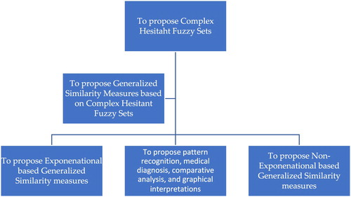
4. To examine the reliability and validity of the proposed measures by comparing with existing measures. The advantages, comparative analysis, and graphical representation of the explored measures and existing measures are also discussed in detail. The graphical interpretation of the explored works is discussed with the help of Figure 1.

Figure 1. The geometrical representation of the explored approach.

The remainder of this manuscript is organized as follows: In Section 2, the notion of FSs, CFSs, HFSs are review. In Section 3, the purpose of this manuscript is to explore the notion of the complex hesitant fuzzy set (CHFS), as a mixture of the hesitant fuzzy set (HFS) and complex fuzzy set (CFS) to cope with the uncertain and complicated information in the real-world decision. CHFS contains truth grades in the form of a subset of the unit disc in a complex plane. The operational laws of the explored notion are also described. In Section 4, the exponential based similarity measures, without exponential based similarity measures, generalized similarity measures, and their important characteristics are also explored. In Section 5, these similarity measures are applied in the environment of pattern recognition and medical diagnosis to evaluate the proficiency and feasibility of the established measures. We solve some numerical examples using the established measures. To examine the reliability and validity of the proposed measures by comparing it with existing measures. The advantages, comparative analysis, and graphical representation of the explored measures and existing measures are also discussed in detail. The conclusion of this manuscript is discussed in Section 6.

2. Preliminaries

In this part of the article, we review basic definitions like FS, CFS, and HFS. Throughout this article $X$ represents a fix set.

Definition 1

[1]: A FS $E$ is of the form: $E=\left\{\left(x,{\mu }_E\left(x\right)\right)|x\in X\right\}$ with a condition $0\le {\mu }_E\left(x\right)\le 1$, where ${\mu }_E\left(x\right)$ represents the grade of truth. Throughout this article, the collection of all FSs on $X$ are denoted by $FS\left(X\right)$. The pair $E=\left(x,{\mu }_E\left(x\right)\right)$ is called fuzzy number (FN).

Definition 2

[16]: A CFS $E$ is of the form: $E=\left\{(x,{\mu }_E\left(x\right)|x\in X\right\}$ where ${\mu }_E\left(x\right)={\gamma }_E\left(x\right).e^{i2\pi \left({\omega }_{{\gamma }_E}\left(x\right)\right)}$ represents the complex-valued truth grade in the form of polar coordinate, where ${\gamma }_E\left(x\right),{\omega }_{{\gamma }_E}\left(x\right)\in \left[0,1\right]$. Further, the pair $E=\left(x,{\gamma }_E\left(x\right).e^{i2\pi \left({\omega }_{{\gamma }_E}\left(x\right)\right)}\right)$ is called complex fuzzy number (CFN).

Definition 3

[24]: A HFS $E$ is of the form: $E=\left\{\left(x,{\mu }_E\left(x\right)\right)|x\in X\right\}$ where ${\mu }_E\left(x\right)$is the set of different finite values in $\left[0,1\right]$ representing the grade of truth for each element $x\in X$. Further, the pair $E=\left(x,{\mu }_E\left(x\right)\right)$ is called hesitant fuzzy number (HFN).

Definition 4

[25]: For any two HFSs $E$ and $F$, the similarity measure $S\left(E,F\right)$ satisfies the following conditions:

1. $0\le S\left(E,F\right)\le 1$;

2. $S\left(E,F\right)=1\iff E=F$;

3. $S\left(E,F\right)=S\left(F,E\right)$.

Definition 5

[25]: For any two HFSs $E$ and $F$, the distance measure $d\left(E,F\right)$ satisfies the following conditions:

1. $0\le d\left(E,F\right)\le 1$;

2. $d\left(E,F\right)=1\iff E=F$;

3. $d\left(E,F\right)=d\left(F,E\right)$.

From the above analysis, we obtain that the $S\left(E,F\right)=1-d\left(E,F\right)$.

3. Complex Hesitant Fuzzy Sets

In this portion, we presented the idea of complex hesitant fuzzy sets (CHFSs) and its some properties.

Definition 6:

A CHFS $E$ is of the form: $E=\text{{ }\left(x,{\mu }_E\left(x\right)\right)\text{|}x\in X\}$ where $\begin{array}{rl}{\mu }_E\left(x\right)& =\left\{{\gamma }_{E_j}\left(x\right).e^{i2\pi \left({\omega }_{{{\gamma }_E}_j}\left(x\right)\right)},j=1,2,3,\dots ,n\right\}\\ & =\left\{{\gamma }_{E_1}\left(x\right).e^{i2\pi \left({\omega }_{{{\gamma }_E}_1}\left(x\right)\right)},{\gamma }_{E_2}\left(x\right).e^{i2\pi \left({\omega }_{{{\gamma }_E}_2}\left(x\right)\right)},\dots ,{\gamma }_{E_n}\left(x\right).e^{i2\pi \left({\omega }_{{{\gamma }_E}_n}\left(x\right)\right)}\right\}\end{array}$ represented the complex-valued truth grade which is subset of unit disc in complex plane with a condition ${\gamma }_{E_j}\left(x\right),{\omega }_{{{\gamma }_E}_j}\left(x\right)\in \left[0,1\right]$. Further, $E=\left(x,{\gamma }_{E_j}\left(x\right).e^{i2\pi \left({\omega }_{{{\gamma }_E}_j}\left(x\right)\right)}\right)$ is called complex hesitant fuzzy number (CHFN).

Definition 7:

Let $E=\left(x,{\gamma }_{E_j}\left(x\right).e^{i2\pi \left({\omega }_{{\gamma }_{E_j}}\left(x\right)\right)}\right)$ and $F=\left(x,{\gamma }_{F_j}\left(x\right).e^{i2\pi \left({\omega }_{{\gamma }_{F_j}}\left(x\right)\right)}\right)$ be two CHFNs. Then

1. $c\left({\gamma }_E\left(x\right)\right)=\left\{\left(x,\left\{1-{\gamma }_{E_j}\left(x\right)\right\}.e^{i2\pi \left(\left\{1-{\omega }_{{{\gamma }_E}_j}\left(x\right)\right\}\right)}\right)\right\}$;

2. $E\cup F=\left\{\left(x,max\left({\gamma }_{E_j}\left(x\right),{\gamma }_{F_j}\left(x\right)\right).e^{i2\pi \left(max\left({\omega }_{{\gamma }_{E_j}}\left(x\right),{\omega }_{{\gamma }_{F_j}}\left(x\right)\right)\right)}\right)\right\}$;

3. $E\cap F=\left\{\left(x,min\left({\gamma }_{E_j}\left(x\right),{\gamma }_{F_j}\left(x\right)\right).e^{i2\pi \left(min\left({\omega }_{{\gamma }_{E_j}}\left(x\right),{\omega }_{{\gamma }_{F_j}}\left(x\right)\right)\right)}\right)\right\}$.

The notion of CHFS is an extensive powerful technique to cope with uncertain and awkward information in realistic decision theory. The CHFS contains the grade of supporting in the form of a subset of the unit disc in the complex plane, whose entities in the form of polar coordinates. Basically, the CHFS contains two-dimension information in a single set. The presented CHFS is more general than existing drawbacks, whose detailed and justifications are discussed are below:

In Definitions (6) and (7), if we choose the imaginary parts as zero, then the explored notion is converted for HFS, which is presented by Torra [24]. Similarly, if we choose the CHFS as a singleton set, then the CHFS is converted for CFS, which is presented by Ramot et al. [16]. Further, if we choose the CHFs as a singleton set and the imaginary part is zero, then the CHFS is converted for FS, which is explored by Zadeh [1]. Due to its structure, it makes powerful and proficient to cope with uncertain and unreliable information in real decision theory.

Example 1:

Let $E=\left\{\begin{array}{c}\left(x_1,\left\{0.9e^{i2\pi \left(0.3\right)},0.7e^{i2\pi \left(0.6\right)}\right\}\right),\left(x_2,\left\{0.3e^{i2\pi \left(0.4\right)},0.8e^{i2\pi \left(0.5\right)},0.5e^{i2\pi \left(0.6\right)}\right\}\right),\\ \left(x_3,\left\{0.6e^{i2\pi \left(0.8\right)}\right\}\right),\left(x_4,\left\{0.7e^{i2\pi \left(0.5\right)},0.9e^{i2\pi \left(0.1\right)},0.3e^{i2\pi \left(0.6\right)}\right\}\right)\end{array}\right\}$ and $F=\left\{\begin{array}{c}\left(x_1,\left\{0.8e^{i2\pi \left(0.6\right)},0.1e^{i2\pi \left(1\right)}\right\}\right),\left(x_2,\left\{0.2e^{i2\pi \left(0.3\right)}\right\}\right),\\ \left(x_3,\left\{0.6e^{i2\pi \left(0.5\right)},0.7e^{i2\pi \left(0.8\right)}\right\}\right),\left(x_4,\left\{1e^{i2\pi \left(0.5\right)},0.7e^{i2\pi \left(0.6\right)},0.9e^{i2\pi \left(0.2\right)}\right\}\right)\end{array}\right\},$ be two CHFSs. Then the operational laws are defined as

1. $E^c=\left\{\begin{array}{c}\left\{0.1e^{i2\pi \left(0.7\right)},0.3e^{i2\pi \left(0.4\right)}\right\},\left\{0.7e^{i2\pi \left(0.6\right)},0.2e^{i2\pi \left(0.5\right)},0.5e^{i2\pi \left(0.4\right)}\right\},\\ \left\{0.4e^{i2\pi \left(0.2\right)}\right\},\left\{0.3e^{i2\pi \left(0.5\right)},0.1e^{i2\pi \left(0.9\right)},0.7e^{i2\pi \left(0.4\right)}\right\}\end{array}\right\};$

2. $E\cup F=\left\{\begin{array}{c}\left\{0.9e^{i2\pi \left(0.6\right)},0.7e^{i2\pi \left(1\right)}\right\},\left\{0.3e^{i2\pi \left(0.4\right)},0.8e^{i2\pi \left(0.5\right)},0.5e^{i2\pi \left(0.6\right)}\right\},\\ \left\{0.6e^{i2\pi \left(0.8\right)},0.7e^{i2\pi \left(0.8\right)}\right\},\left\{1e^{i2\pi \left(0.5\right)},0.9e^{i2\pi \left(0.6\right)},0.9e^{i2\pi \left(0.6\right)}\right\}\end{array}\right\};$ $E\cap F=\left\{\begin{array}{c}\left\{0.8e^{i2\pi \left(0.3\right)},0.1e^{i2\pi \left(0.6\right)}\right\},\left\{0.2e^{i2\pi \left(0.3\right)}\right\},\\ \left\{0.6e^{i2\pi \left(0.5\right)}\right\},\left\{0.7e^{i2\pi \left(0.5\right)},0.7e^{i2\pi \left(0.1\right)},0.3e^{i2\pi \left(0.2\right)}\right\}\end{array}\right\}.$

Theorem 1:

Let $E,F$ and $G\in CHFS\left(X\right)$ then the following holds

1. $c\left(c\left(E\right)\right)=E$

2. i. $E\cup F=F\cup E$ii. $E\cap F=F\cap E$

3. i. $\left(E\cup F\right)\cup G=E\cup \left(F\cup G\right)$

   ii. $\left(E\cap F\right)\cap G=E\cap \left(F\cap G\right)$

4. $E\cup \left(F\cap G\right)=\left(E\cup F\right)\cap \left(E\cup G\right)$

5. $E\cap \left(F\cup G\right)=\left(E\cap F\right)\cup \left(E\cap G\right)$

Proof:

In this theorem we have $E=\left(x,{\gamma }_{E_j}\left(x\right).e^{i2\pi \left({\omega }_{{{\gamma }_E}_j}\left(x\right)\right)}\right)$, $F=\left(x,{\gamma }_{F_j}\left(x\right).e^{i2\pi \left({\omega }_{{\gamma }_{F_j}}\left(x\right)\right)}\right)$ and $G=\left(x,{\gamma }_{G_j}\left(x\right).e^{i2\pi \left({\omega }_{{\gamma }_{G_j}}\left(x\right)\right)}\right)$

1. By Definition $7$ we have $\begin{array}{rl}c\left(E\right)& =c\left(x,{\gamma }_{E_j}\left(x\right).e^{i2\pi \left({\omega }_{{{\gamma }_E}_j}\left(x\right)\right)}\right)=\left\{\left(x,\left\{1-{\gamma }_{E_j}\left(x\right)\right\}.e^{i2\pi \left(\left\{1-{\omega }_{{{\gamma }_E}_j}\left(x\right)\right\}\right)}\right)\right\},\text{then}\\ c\left(c\left(E\right)\right)& =\left\{\left(x,\left\{1-\left(1-{\gamma }_{E_j}\left(x\right)\right)\right\}.e^{i2\pi \left(\left\{1-\left(1-{\omega }_{{{\gamma }_E}_j}\left(x\right)\right)\right\}\right)}\right)\right\}\\ & =\left(x,{\gamma }_{E_j}\left(x\right).e^{i2\pi \left({\omega }_{{{\gamma }_E}_j}\left(x\right)\right)}\right)=E.\end{array}$

2. By Definition $7$ we have $\begin{array}{rl}E\cup F& =\left\{\left(x,max\left({\gamma }_{E_j}\left(x\right),{\gamma }_{F_j}\left(x\right)\right).e^{i2\pi \left(max\left({\omega }_{{\gamma }_{E_j}}\left(x\right),{\omega }_{{\gamma }_{F_j}}\left(x\right)\right)\right)}\right)\right\}\\ & =\left\{\left(x,max\left({\gamma }_{F_j}\left(x\right),{\gamma }_{E_j}\left(x\right)\right).e^{i2\pi \left(max\left({\omega }_{{\gamma }_{F_j}}\left(x\right),{\omega }_{{\gamma }_{E_j}}\left(x\right)\right)\right)}\right)\right\}\\ & =F\cup E.\end{array}$ $\begin{array}{rl}E\cap F& =\left\{\left(x,min\left({\gamma }_{E_j}\left(x\right),{\gamma }_{F_j}\left(x\right)\right).e^{i2\pi \left(min\left({\omega }_{{\gamma }_{E_j}}\left(x\right),{\omega }_{{\gamma }_{F_j}}\left(x\right)\right)\right)}\right)\right\}\\ & =\left\{\left(x,min\left({\gamma }_{F_j}\left(x\right),{\gamma }_{E_j}\left(x\right)\right).e^{i2\pi \left(min\left({\omega }_{{\gamma }_{F_j}}\left(x\right),{\omega }_{{\gamma }_{E_j}}\left(x\right)\right)\right)}\right)\right\}\\ & =F\cap E\end{array}$

3. i. By Definition $7$ we have $E\cup F=\left\{\left(x,max\left({\gamma }_{E_j}\left(x\right),{\gamma }_{F_j}\left(x\right)\right).e^{i2\pi \left(max\left({\omega }_{{\gamma }_{E_j}}\left(x\right),{\omega }_{{\gamma }_{F_j}}\left(x\right)\right)\right)}\right)\right\}$

To prove that $\left(E\cup F\right)\cup G=E\cup \left(F\cup G\right)$. As $\begin{array}{rl}E\cup F& =\left\{\left(x,max\left({\gamma }_{E_j}\left(x\right),{\gamma }_{F_j}\left(x\right)\right).e^{i2\pi \left(max\left({\omega }_{{\gamma }_{E_j}}\left(x\right),{\omega }_{{\gamma }_{F_j}}\left(x\right)\right)\right)}\right)\right\}\text{then}\\ \left(E\cup F\right)\cup G& =\left\{\left(x,max\left(\text{max}\left({\gamma }_{E_j}\left(x\right),{\gamma }_{F_j}\left(x\right)\right),{\gamma }_{G_j}\left(x\right)\right).e^{i2\pi \left(max\left(\text{max}\left({\omega }_{{\gamma }_{E_j}}\left(x\right),{\omega }_{{\gamma }_{F_j}}\left(x\right)\right),{\omega }_{{\gamma }_{G_j}}\left(x\right)\right)\right)}\right)\right\}\\ & =\left\{\left(x,max\left({\gamma }_{E_j}\left(x\right),\text{max}\left({\gamma }_{F_j}\left(x\right),{\gamma }_{G_j}\left(x\right)\right)\right).e^{i2\pi \left(max\left({\omega }_{{\gamma }_{E_j}}\left(x\right),\text{max}\left({\omega }_{{\gamma }_{F_j}}\left(x\right),{\omega }_{{\gamma }_{G_j}}\left(x\right)\right)\right)\right)}\right)\right\}\\ & =E\cup \left(F\cup G\right).\end{array}$   ii. By Definition $7$ we have $E\cap F=\left\{\left(x,min\left({\gamma }_{E_j}\left(x\right),{\gamma }_{F_j}\left(x\right)\right).e^{i2\pi \left(min\left({\omega }_{{\gamma }_{E_j}}\left(x\right),{\omega }_{{\gamma }_{F_j}}\left(x\right)\right)\right)}\right)\right\}$ To prove that $\left(E\cap F\right)\cap G=E\cap \left(F\cap G\right)$. As $\begin{array}{rl}E\cap F& =\left\{\left(x,min\left({\gamma }_{E_j}\left(x\right),{\gamma }_{F_j}\left(x\right)\right).e^{i2\pi \left(min\left({\omega }_{{\gamma }_{E_j}}\left(x\right),{\omega }_{{\gamma }_{F_j}}\left(x\right)\right)\right)}\right)\right\}\text{then}\\ \left(E\cap F\right)\cap G& =\left\{\left(x,min\left(\text{min}\left({\gamma }_{E_j}\left(x\right),{\gamma }_{F_j}\left(x\right)\right),{\gamma }_{G_j}\left(x\right)\right).e^{i2\pi \left(min\left(\text{min}\left({\omega }_{{\gamma }_{E_j}}\left(x\right),{\omega }_{{\gamma }_{F_j}}\left(x\right)\right),{\omega }_{{\gamma }_{G_j}}\left(x\right)\right)\right)}\right)\right\}\\ & =\left\{\left(x,min\left({\gamma }_{E_j}\left(x\right),\text{min}\left({\gamma }_{F_j}\left(x\right),{\gamma }_{G_j}\left(x\right)\right)\right).e^{i2\pi \left(min\left({\omega }_{{\gamma }_{E_j}}\left(x\right),\text{min}\left({\omega }_{{\gamma }_{F_j}}\left(x\right),{\omega }_{{\gamma }_{G_j}}\left(x\right)\right)\right)\right)}\right)\right\}\\ & =E\cap \left(F\cap G\right).\end{array}$

(4)	By definition $7$ we have $F\cap G=\left\{\left(x,min\left({\gamma }_{F_j}\left(x\right),{\gamma }_{G_j}\left(x\right)\right).e^{i2\pi \left(min\left({\omega }_{{\gamma }_{F_j}}\left(x\right),{\omega }_{{\gamma }_{G_j}}\left(x\right)\right)\right)}\right)\right\}$

Then $E\cup \left(F\cap G\right)=\left\{\left(x,max\left({\gamma }_{E_j}\left(x\right),\text{min}\left({\gamma }_{F_j}\left(x\right),{\gamma }_{G_j}\left(x\right)\right)\right).e^{i2\pi \left(max\left({\omega }_{{\gamma }_{E_j}}\left(x\right),\text{min}\left({\omega }_{{\gamma }_{F_j}}\left(x\right),{\omega }_{{\gamma }_{G_j}}\left(x\right)\right)\right)\right)}\right)\right\}$ Next we have $E\cup F=\left\{\left(x,max\left({\gamma }_{E_j}\left(x\right),{\gamma }_{F_j}\left(x\right)\right).e^{i2\pi \left(max\left({\omega }_{{\gamma }_{E_j}}\left(x\right),{\omega }_{{\gamma }_{F_j}}\left(x\right)\right)\right)}\right)\right\}$ and $E\cup G=\left\{\left\{\left(x,max\left({\gamma }_{E_j}\left(x\right),{\gamma }_{G_j}\left(x\right)\right).e^{i2\pi \left(max\left({\omega }_{{\gamma }_{E_j}}\left(x\right),{\omega }_{{\gamma }_{G_j}}\left(x\right)\right)\right)}\right)\right\}\right\}$ then $\begin{array}{rl}& \left(E\cup F\right)\cap \left(E\cup G\right)\\ & =\left\{\left(x,min\left(\begin{array}{c}max\left({\gamma }_{E_j}\left(x\right),{\gamma }_{F_j}\left(x\right)\right),\\ max\left({\gamma }_{E_j}\left(x\right),{\gamma }_{G_j}\left(x\right)\right)\end{array}\right).e^{i2\pi \left(min\left(\begin{array}{c}max\left({\omega }_{{\gamma }_{E_j}}\left(x\right),{\omega }_{{\gamma }_{F_j}}\left(x\right)\right),\\ max\left({\omega }_{{\gamma }_{E_j}}\left(x\right),{\omega }_{{\gamma }_{G_j}}\left(x\right)\right)\end{array}\right)\right)}\right)\right\}\\ & =\left\{\left(x,max\left({\gamma }_{E_j}\left(x\right),\text{min}\left({\gamma }_{F_j}\left(x\right),{\gamma }_{G_j}\left(x\right)\right)\right).e^{i2\pi \left(max\left({\omega }_{{\gamma }_{E_j}}\left(x\right),\text{min}\left({\omega }_{{\gamma }_{F_j}}\left(x\right),{\omega }_{{\gamma }_{G_j}}\left(x\right)\right)\right)\right)}\right)\right\}\end{array}$ Finally we obtain $E\cup \left(F\cap G\right)=\left(E\cup F\right)\cap \left(E\cup G\right).$

(5)	By Definition $7$ we have $F\cup G=\left\{\left(x,max\left({\gamma }_{F_j}\left(x\right),{\gamma }_{G_j}\left(x\right)\right).e^{i2\pi \left(max\left({\omega }_{{\gamma }_{F_j}}\left(x\right),{\omega }_{{\gamma }_{G_j}}\left(x\right)\right)\right)}\right)\right\}$

Then $E\cap \left(F\cup G\right)=\left\{\left(x,min\left({\gamma }_{E_j}\left(x\right),\text{max}\left({\gamma }_{F_j}\left(x\right),{\gamma }_{G_j}\left(x\right)\right)\right).e^{i2\pi \left(min\left({\omega }_{{\gamma }_{E_j}}\left(x\right),\text{max}\left({\omega }_{{\gamma }_{F_j}}\left(x\right),{\omega }_{{\gamma }_{G_j}}\left(x\right)\right)\right)\right)}\right)\right\}$ Next we have $E\cap F=\left\{\left(x,min\left({\gamma }_{E_j}\left(x\right),{\gamma }_{F_j}\left(x\right)\right).e^{i2\pi \left(min\left({\omega }_{{\gamma }_{E_j}}\left(x\right),{\omega }_{{\gamma }_{F_j}}\left(x\right)\right)\right)}\right)\right\}.$ and $E\cap G=\left\{\left(x,min\left({\gamma }_{E_j}\left(x\right),{\gamma }_{G_j}\left(x\right)\right).e^{i2\pi \left(min\left({\omega }_{{\gamma }_{e_j}}\left(x\right),{\omega }_{{\gamma }_{G_j}}\left(x\right)\right)\right)}\right)\right\}$ then $\begin{array}{rl}& \left(E\cap F\right)\cup \left(E\cap G\right)\\ & =\left\{\left(x,max\left(\begin{array}{c}min\left({\gamma }_{E_j}\left(x\right),{\gamma }_{F_j}\left(x\right)\right),\\ min\left({\gamma }_{E_j}\left(x\right),{\gamma }_{G_j}\left(x\right)\right)\end{array}\right).e^{i2\pi \left(max\left(\begin{array}{c}min\left({\omega }_{{\gamma }_{E_j}}\left(x\right),{\omega }_{{\gamma }_{F_j}}\left(x\right)\right),\\ min\left({\omega }_{{\gamma }_{E_j}}\left(x\right),{\omega }_{{\gamma }_{G_j}}\left(x\right)\right)\end{array}\right)\right)}\right)\right\}\\ & =\left\{\left(x,min\left({\gamma }_{E_j}\left(x\right),\text{max}\left({\gamma }_{F_j}\left(x\right),{\gamma }_{G_j}\left(x\right)\right)\right).e^{i2\pi \left(min\left({\omega }_{{\gamma }_{E_j}}\left(x\right),\text{max}\left({\omega }_{{\gamma }_{F_j}}\left(x\right),{\omega }_{{\gamma }_{G_j}}\left(x\right)\right)\right)\right)}\right)\right\}\end{array}$ Finally we obtain $E\cup \left(F\cap G\right)=\left(E\cup F\right)\cap \left(E\cup G\right).$

Example 2:

Let $E=\left\{\begin{array}{c}\left(x_1,\left\{0.9e^{i2\pi \left(0.3\right)},0.7e^{i2\pi \left(0.6\right)}\right\}\right),\left(x_2,\left\{0.3e^{i2\pi \left(0.4\right)},0.8e^{i2\pi \left(0.5\right)},0.5e^{i2\pi \left(0.6\right)}\right\}\right),\\ \left(x_3,\left\{0.6e^{i2\pi \left(0.8\right)}\right\}\right),\left(x_4,\left\{0.7e^{i2\pi \left(0.5\right)},0.9e^{i2\pi \left(0.1\right)},0.3e^{i2\pi \left(0.6\right)}\right\}\right)\end{array}\right\}$ $F=\left\{\begin{array}{c}\left(x_1,\left\{0.8e^{i2\pi \left(0.6\right)},0.1e^{i2\pi \left(1\right)}\right\}\right),\left(x_2,\left\{0.2e^{i2\pi \left(0.3\right)}\right\}\right),\\ \left(x_3,\left\{0.6e^{i2\pi \left(0.5\right)},0.7e^{i2\pi \left(0.8\right)}\right\}\right),\left(x_4,\left\{1e^{i2\pi \left(0.5\right)},0.7e^{i2\pi \left(0.6\right)},0.9e^{i2\pi \left(0.2\right)}\right\}\right)\end{array}\right\},$and $G=\left\{\begin{array}{c}\left(x_1,\left\{0.2e^{i2\pi \left(0.1\right)},0.7e^{i2\pi \left(0.1\right)}\right\}\right),\left(x_2,\left\{0.3e^{i2\pi \left(0.9\right)},1e^{i2\pi \left(0.4\right)}\right\}\right),\\ \left(x_3,\left\{0.9e^{i2\pi \left(0.8\right)},0.4e^{i2\pi \left(0.2\right)}\right\}\right),\left(x_4,\left\{0.7e^{i2\pi \left(0.6\right)},0.8e^{i2\pi \left(0.3\right)},0.9e^{i2\pi \left(1\right)}\right\}\right)\end{array}\right\}$ be CHFSs. Then

1. $c\left(E\right)=\left\{\begin{array}{c}\left\{0.1e^{i2\pi \left(0.7\right)},0.3e^{i2\pi \left(0.4\right)}\right\},\left\{0.3e^{i2\pi \left(0.4\right)},0.8e^{i2\pi \left(0.5\right)},0.5e^{i2\pi \left(0.6\right)}\right\},\\ \left\{0.4e^{i2\pi \left(0.2\right)}\right\},\left\{0.3e^{i2\pi \left(0.5\right)},0.1e^{i2\pi \left(0.9\right)},0.7e^{i2\pi \left(0.4\right)}\right\}\end{array}\right\}$;

2. $c\left(c\left(E\right)\right)=\left\{\begin{array}{c}\left\{0.9e^{i2\pi \left(0.3\right)},0.7e^{i2\pi \left(0.6\right)}\right\},\left\{0.7e^{i2\pi \left(0.6\right)},0.2e^{i2\pi \left(0.5\right)},0.5e^{i2\pi \left(0.4\right)}\right\},\\ \left\{0.6e^{i2\pi \left(0.8\right)}\right\},\left\{0.7e^{i2\pi \left(0.5\right)},0.9e^{i2\pi \left(0.1\right)},0.3e^{i2\pi \left(0.6\right)}\right\}\end{array}\right\}$;

3. i. $E\cup F=\left\{\begin{array}{c}\left\{0.9e^{i2\pi \left(0.6\right)},0.7e^{i2\pi \left(1\right)}\right\},\left\{0.3e^{i2\pi \left(0.4\right)},0.8e^{i2\pi \left(0.5\right)},0.5e^{i2\pi \left(0.6\right)}\right\},\\ \left\{0.6e^{i2\pi \left(0.8\right)},0.7e^{i2\pi \left(0.8\right)}\right\},\left\{1e^{i2\pi \left(0.5\right)},0.9e^{i2\pi \left(0.6\right)},0.9e^{i2\pi \left(0.6\right)}\right\}\end{array}\right\}$

and $E\cup F=\left\{\begin{array}{c}\left\{0.9e^{i2\pi \left(0.6\right)},0.7e^{i2\pi \left(1\right)}\right\},\left\{0.3e^{i2\pi \left(0.4\right)},0.8e^{i2\pi \left(0.5\right)},0.5e^{i2\pi \left(0.6\right)}\right\},\\ \left\{0.6e^{i2\pi \left(0.8\right)},0.7e^{i2\pi \left(0.8\right)}\right\},\left\{1e^{i2\pi \left(0.5\right)},0.9e^{i2\pi \left(0.6\right)},0.9e^{i2\pi \left(0.6\right)}\right\}\end{array}\right\}$ this implies that $E\cup F=F\cup E$.

   ii. $E\cap F=\left\{\begin{array}{c}\left\{0.8e^{i2\pi \left(0.3\right)},0.1e^{i2\pi \left(0.6\right)}\right\},\left\{0.2e^{i2\pi \left(0.3\right)}\right\},\\ \left\{0.6e^{i2\pi \left(0.5\right)}\right\},\left\{0.7e^{i2\pi \left(0.5\right)},0.7e^{i2\pi \left(0.1\right)},0.3e^{i2\pi \left(0.2\right)}\right\}\end{array}\right\}$

and $F\cap E=\left\{\begin{array}{c}\left\{0.8e^{i2\pi \left(0.3\right)},0.1e^{i2\pi \left(0.6\right)}\right\},\left\{0.2e^{i2\pi \left(0.3\right)}\right\},\\ \left\{0.6e^{i2\pi \left(0.5\right)}\right\},\left\{0.7e^{i2\pi \left(0.5\right)},0.7e^{i2\pi \left(0.1\right)},0.3e^{i2\pi \left(0.2\right)}\right\}\end{array}\right\}$ this implies that $E\cap F=F\cap E$.

(4)

i. We have $\left(E\cup F\right)\cup G=\left\{\begin{array}{c}\left\{0.9e^{i2\pi \left(0.6\right)},0.7e^{i2\pi \left(1\right)}\right\},\left\{0.3e^{i2\pi \left(0.9\right)},1e^{i2\pi \left(0.5\right)},0.5e^{i2\pi \left(0.6\right)}\right\},\\ \left\{0.9e^{i2\pi \left(0.8\right)},0.7e^{i2\pi \left(0.8\right)}\right\},\left\{1e^{i2\pi \left(0.6\right)},0.9e^{i2\pi \left(0.6\right)},0.9e^{i2\pi \left(1\right)}\right\}\end{array}\right\}$

And $F\cup G=\left\{\begin{array}{c}\left\{0.8e^{i2\pi \left(0.6\right)},0.7e^{i2\pi \left(1\right)}\right\},\left\{0.3e^{i2\pi \left(0.9\right)},1e^{i2\pi \left(0.4\right)}\right\},\\ \left\{0.9e^{i2\pi \left(0.8\right)},0.7e^{i2\pi \left(0.8\right)}\right\},\left\{1e^{i2\pi \left(0.6\right)},0.8e^{i2\pi \left(0.6\right)},0.9e^{i2\pi \left(1\right)}\right\}\end{array}\right\}$ This implies that $E\cup \left(F\cup G\right)=\left\{\begin{array}{c}\left\{0.9e^{i2\pi \left(0.6\right)},0.7e^{i2\pi \left(1\right)}\right\},\left\{0.3e^{i2\pi \left(0.9\right)},1e^{i2\pi \left(0.5\right)},0.5e^{i2\pi \left(0.6\right)}\right\},\\ \left\{0.9e^{i2\pi \left(0.8\right)},0.7e^{i2\pi \left(0.8\right)}\right\},\left\{1e^{i2\pi \left(0.6\right)},0.9e^{i2\pi \left(0.6\right)},0.9e^{i2\pi \left(1\right)}\right\}\end{array}\right\}$ Finally we obtain $\left(E\cup F\right)\cup G=E\cup \left(F\cup G\right).$    ii. Next we have $\left(E\cap F\right)\cap G=\left\{\begin{array}{c}\left\{0.2e^{i2\pi \left(0.1\right)},0.1e^{i2\pi \left(0.1\right)}\right\},\left\{0.2e^{i2\pi \left(0.3\right)}\right\},\\ \left\{0.6e^{i2\pi \left(0.5\right)}\right\},\left\{0.7e^{i2\pi \left(0.5\right)},0.7e^{i2\pi \left(0.1\right)},0.3e^{i2\pi \left(0.2\right)}\right\}\end{array}\right\}$ And $F\cap G=\left\{\begin{array}{c}\left\{0.2e^{i2\pi \left(0.1\right)},0.1e^{i2\pi \left(0.1\right)}\right\},\left\{0.2e^{i2\pi \left(0.3\right)}\right\},\\ \left\{0.6e^{i2\pi \left(0.5\right)},0.4e^{i2\pi \left(0.2\right)}\right\},\left\{0.7e^{i2\pi \left(0.5\right)},0.7e^{i2\pi \left(0.3\right)},0.9e^{i2\pi \left(0.2\right)}\right\}\end{array}\right\}$ This implies that $E\cap \left(F\cap G\right)=\left\{\begin{array}{c}\left\{0.2e^{i2\pi \left(0.1\right)},0.1e^{i2\pi \left(0.1\right)}\right\},\left\{0.2e^{i2\pi \left(0.3\right)}\right\},\\ \left\{0.6e^{i2\pi \left(0.5\right)}\right\},\left\{0.7e^{i2\pi \left(0.5\right)},0.7e^{i2\pi \left(0.1\right)},0.3e^{i2\pi \left(0.2\right)}\right\}\end{array}\right\}$ Finally we obtain $\left(E\cap F\right)\cap G=E\cap \left(F\cap G\right).$

(5)

We have $F\cap G=\left\{\begin{array}{c}\left\{0.2e^{i2\pi \left(0.1\right)},0.1e^{i2\pi \left(0.1\right)}\right\},\left\{0.2e^{i2\pi \left(0.3\right)}\right\},\\ \left\{0.6e^{i2\pi \left(0.5\right)},0.4e^{i2\pi \left(0.2\right)}\right\},\left\{0.7e^{i2\pi \left(0.5\right)},0.7e^{i2\pi \left(0.3\right)},0.9e^{i2\pi \left(0.2\right)}\right\}\end{array}\right\}$

Then $E\cup \left(F\cap G\right)=\left\{\begin{array}{c}\left(x_1,\left\{0.9e^{i2\pi \left(0.3\right)},0.7e^{i2\pi \left(0.6\right)}\right\}\right),\left(x_2,\left\{0.3e^{i2\pi \left(0.4\right)},0.8e^{i2\pi \left(0.5\right)},0.5e^{i2\pi \left(0.6\right)}\right\}\right),\\ \left(x_3,\left\{0.6e^{i2\pi \left(0.8\right)},0.4e^{i2\pi \left(0.2\right)}\right\}\right),\left(x_4,\left\{0.7e^{i2\pi \left(0.5\right)},0.9e^{i2\pi \left(0.3\right)},0.9e^{i2\pi \left(0.6\right)}\right\}\right)\end{array}\right\}$ Next we have $E\cup F=\left\{\begin{array}{c}\left\{0.9e^{i2\pi \left(0.6\right)},0.7e^{i2\pi \left(1\right)}\right\},\left\{0.3e^{i2\pi \left(0.4\right)},0.8e^{i2\pi \left(0.5\right)},0.5e^{i2\pi \left(0.6\right)}\right\},\\ \left\{0.6e^{i2\pi \left(0.8\right)},0.7e^{i2\pi \left(0.8\right)}\right\},\left\{1e^{i2\pi \left(0.5\right)},0.9e^{i2\pi \left(0.6\right)},0.9e^{i2\pi \left(0.6\right)}\right\}\end{array}\right\}$ and $E\cup G=\left\{\begin{array}{c}\left(x_1,\left\{0.9e^{i2\pi \left(0.3\right)},0.7e^{i2\pi \left(0.6\right)}\right\}\right),\left(x_2,\left\{0.3e^{i2\pi \left(0.9\right)},1e^{i2\pi \left(0.5\right)},0.5e^{i2\pi \left(0.6\right)}\right\}\right),\\ \left(x_3,\left\{0.9e^{i2\pi \left(0.8\right)},0.4e^{i2\pi \left(0.2\right)}\right\}\right),\left(x_4,\left\{0.7e^{i2\pi \left(0.6\right)},0.9e^{i2\pi \left(0.3\right)},0.9e^{i2\pi \left(1\right)}\right\}\right)\end{array}\right\}$ then $\left(E\cup F\right)\cap \left(E\cup G\right)=\left\{\begin{array}{c}\left\{0.9e^{i2\pi \left(0.3\right)},0.7e^{i2\pi \left(0.6\right)}\right\},\left\{0.3e^{i2\pi \left(0.4\right)},0.8e^{i2\pi \left(0.5\right)},0.5e^{i2\pi \left(0.6\right)}\right\},\\ \left\{0.6e^{i2\pi \left(0.8\right)},0.4e^{i2\pi \left(0.2\right)}\right\},\left\{0.7e^{i2\pi \left(0.5\right)},0.9e^{i2\pi \left(0.3\right)},0.9e^{i2\pi \left(0.6\right)}\right\}\end{array}\right\}$ Finally we obtain $E\cup \left(F\cap G\right)=\left(E\cup F\right)\cap \left(E\cup G\right).$

(6)

We have $F\cup G=\left\{\begin{array}{c}\left\{0.8e^{i2\pi \left(0.6\right)},0.7e^{i2\pi \left(1\right)}\right\},\left\{0.3e^{i2\pi \left(0.9\right)},1e^{i2\pi \left(0.4\right)}\right\},\\ \left\{0.9e^{i2\pi \left(0.8\right)},0.7e^{i2\pi \left(0.8\right)}\right\},\left\{1e^{i2\pi \left(0.6\right)},0.8e^{i2\pi \left(0.6\right)},0.9e^{i2\pi \left(1\right)}\right\}\end{array}\right\}$

Then $E\cap \left(F\cup G\right)=\left\{\begin{array}{c}\left\{0.8e^{i2\pi \left(0.6\right)},0.7e^{i2\pi \left(1\right)}\right\},\left\{0.3e^{i2\pi \left(0.4\right)},0.8e^{i2\pi \left(0.4\right)}\right\},\\ \left\{0.6e^{i2\pi \left(0.8\right)}\right\},\left\{0.7e^{i2\pi \left(0.5\right)},0.8e^{i2\pi \left(0.1\right)},0.3e^{i2\pi \left(0.6\right)}\right\}\end{array}\right\}$ Next we have $E\cap F=\left\{\begin{array}{c}\left\{0.8e^{i2\pi \left(0.3\right)},0.1e^{i2\pi \left(0.6\right)}\right\},\left\{0.2e^{i2\pi \left(0.3\right)}\right\},\\ \left\{0.6e^{i2\pi \left(0.5\right)}\right\},\left\{0.7e^{i2\pi \left(0.5\right)},0.7e^{i2\pi \left(0.1\right)},0.3e^{i2\pi \left(0.2\right)}\right\}\end{array}\right\}$ and $E$ then $\left(E\cap F\right)\cup \left(E\cap G\right)=\left\{\begin{array}{c}\left\{0.8e^{i2\pi \left(0.6\right)},0.7e^{i2\pi \left(1\right)}\right\},\left\{0.3e^{i2\pi \left(0.4\right)},0.8e^{i2\pi \left(0.4\right)}\right\},\\ \left\{0.6e^{i2\pi \left(0.8\right)}\right\},\left\{0.7e^{i2\pi \left(0.5\right)},0.8e^{i2\pi \left(0.1\right)},0.3e^{i2\pi \left(0.6\right)}\right\}\end{array}\right\}$ Finally we obtain $E\cap \left(F\cup G\right)=\left(E\cap F\right)\cup \left(E\cap G\right).$

4. The Generalized Similarity Measures Based on CHFSs

In the part of the paper, we proposed SMs established on the exponential function. We also proposed SMs without exponential function.

Definition 8:

Let $E$ and $F$ be two CHFSs on $X$. Then similarity measure (SM) between $E$ and $F$is identified by $S_c\left(E,F\right)$, which satisfies the following properties

1. $0\le S_c\left(E,F\right)\le 1$;

2. $S_c\left(E,F\right)=1$if and only if $E=F$;

3. $S_c\left(E,F\right)=S_c\left(F,E\right)$.

Definition 9:

Let $E$ and $F$ be two CHFS on $X$. Then the exponential based generalized SM is calculated as $S_c^1\left(E,F\right)={\left[\frac{1}{n}\sum _{k=1}^n\left[2^{1-\left(\frac{1}{\ell }\sum _{j=1}^{\ell }{|{\gamma }_{E_j}\left(x_k\right)-{\gamma }_{F_j}\left(x_k\right)|}^{\lambda }\vee \frac{1}{\ell }\sum _{j=1}^{\ell }{|{\omega }_{{\gamma }_{E_j}}\left(x_k\right)-{\omega }_{{\gamma }_{F_j}}\left(x_k\right)|}^{\lambda }\right)}-1\right]\right]}^{\frac{1}{\lambda }}$ where $\lambda >0$, and $\vee$ described the maximum operation.

In Definitions (8) and (9), if we choose the imaginary parts will be zero, then the explored notion is converted for HFS. Similarly, if we choose the CHFS is a singleton set, then the CHFS is converted for CFS. Further, if we choose the CHFs is a singleton set and the imaginary part will be zero, then the CHFS is converted for FS. Due to its structure, it make powerful and proficient to cope with uncertain and unreliable information in real decision theory.

Theorem 2:

The SM $S_c^1\left(E,F\right)$ satisfy the following properties

1. $0\le S_c^1\left(E,F\right)\le 1$;

2. $S_c^1\left(E,F\right)=1$ if and only if $E=F$;

3. $S_c^1\left(E,F\right)=S_c^1\left(F,E\right)$.

Proof:

1. Since $\frac{1}{\ell }\sum _{j=1}^{\ell }|{\gamma }_{E_j}\left(x_k\right)-{\gamma }_{F_j}\left(x_k\right){|}^{\lambda }\in \left[0,1\right]$ and $\frac{1}{\ell }\sum _{j=1}^{\ell }|{\omega }_{{\gamma }_{E_j}}\left(x_k\right)-{\omega }_{{\gamma }_{F_j}}\left(x_k\right){|}^{\lambda }\in \left[0,1\right]$ then $\frac{1}{\ell }\sum _{j=1}^{\ell }|{\gamma }_{E_j}\left(x_k\right)-{\gamma }_{F_j}\left(x_k\right){|}^{\lambda }\vee \frac{1}{\ell }\sum _{j=1}^{\ell }|{\omega }_{{\gamma }_{E_j}}\left(x_k\right)-{\omega }_{{\gamma }_{F_j}}\left(x_k\right){|}^{\lambda }\in \left[0,1\right]$ this implies that for $k=1$ we have $2^{1-\left(\frac{1}{\ell }\sum _{j=1}^{\ell }{|{\gamma }_{E_j}\left(x_1\right)-{\gamma }_{F_j}\left(x_1\right)|}^{\lambda }\vee \frac{1}{\ell }\sum _{j=1}^{\ell }{|{\omega }_{{\gamma }_{E_j}}\left(x_1\right)-{\omega }_{{\gamma }_{F_j}}\left(x_1\right)|}^{\lambda }\right)}-1\in \left[0,1\right]$ For $k=2$ $2^{1-\left(\frac{1}{\ell }\sum _{j=1}^{\ell }{|{\gamma }_{E_j}\left(x_2\right)-{\gamma }_{F_j}\left(x_2\right)|}^{\lambda }\vee \frac{1}{\ell }\sum _{j=1}^{\ell }{|{\omega }_{{\gamma }_{E_j}}\left(x_2\right)-{\omega }_{{\gamma }_{F_j}}\left(x_2\right)|}^{\lambda }\right)}-1\in \left[0,1\right]$ By doing this process we obtain $\begin{array}{rl}& \sum _{k=1}^n\left[2^{1-\left(\frac{1}{\ell }\sum _{j=1}^{\ell }{|{\gamma }_{E_j}\left(x_k\right)-{\gamma }_{F_j}\left(x_k\right)|}^{\lambda }\vee \frac{1}{\ell }\sum _{j=1}^{\ell }{|{\omega }_{{\gamma }_{E_j}}\left(x_k\right)-{\omega }_{{\gamma }_{F_j}}\left(x_k\right)|}^{\lambda }\right)}-1\right]\in n\left[0,1\right]\\ & \Rightarrow 0\le \sum _{k=1}^n\left[2^{1-\left(\frac{1}{\ell }\sum _{j=1}^{\ell }{|{\gamma }_{E_j}\left(x_k\right)-{\gamma }_{F_j}\left(x_k\right)|}^{\lambda }\vee \frac{1}{\ell }\sum _{j=1}^{\ell }{|{\omega }_{{\gamma }_{E_j}}\left(x_k\right)-{\omega }_{{\gamma }_{F_j}}\left(x_k\right)|}^{\lambda }\right)}-1\right]\le n\\ & \Rightarrow 0\le \frac{1}{n}\sum _{k=1}^n\left[2^{1-\left(\frac{1}{\ell }\sum _{j=1}^{\ell }{|{\gamma }_{E_j}\left(x_k\right)-{\gamma }_{F_j}\left(x_k\right)|}^{\lambda }\vee \frac{1}{\ell }\sum _{j=1}^{\ell }{|{\omega }_{{\gamma }_{E_j}}\left(x_k\right)-{\omega }_{{\gamma }_{F_j}}\left(x_k\right)|}^{\lambda }\right)}-1\right]\le 1\\ & \Rightarrow 0\le {\left[\frac{1}{n}\sum _{k=1}^n\left[2^{1-\left(\frac{1}{\ell }\sum _{j=1}^{\ell }{|{\gamma }_{E_j}\left(x_k\right)-{\gamma }_{F_j}\left(x_k\right)|}^{\lambda }\vee \frac{1}{\ell }\sum _{j=1}^{\ell }{|{\omega }_{{\gamma }_{E_j}}\left(x_k\right)-{\omega }_{{\gamma }_{F_j}}\left(x_k\right)|}^{\lambda }\right)}-1\right]\right]}^{\frac{1}{\lambda }}\le 1\\ & \Rightarrow 0\le S_c^1\left(E,F\right)\le 1.\end{array}$ 2. By Definition 7 we have $\begin{array}{rl}{S}_c^1\left(E,F\right)& ={\left[\frac{1}{n}\sum _{k=1}^n\left[2^{1-\left(\frac{1}{\ell }\sum _{j=1}^{\ell }{|{\gamma }_{E_j}\left(x_k\right)-{\gamma }_{F_j}\left(x_k\right)|}^{\lambda }\vee \frac{1}{\ell }\sum _{j=1}^{\ell }{|{\omega }_{{\gamma }_{E_j}}\left(x_k\right)-{\omega }_{{\gamma }_{F_j}}\left(x_k\right)|}^{\lambda }\right)}-1\right]\right]}^{\frac{1}{\lambda }}\\ \iff S_c^1\left(E,F\right)& ={\left[\frac{1}{n}\sum _{k=1}^n\left[2^{1-\left(\begin{array}{c}\frac{1}{\ell }\left(\left({|{\gamma }_{E_1}\left(x_k\right)-{\gamma }_{F_1}\left(x_k\right)|}^{\lambda }+{|{\gamma }_{E_2}\left(x_k\right)-{\gamma }_{F_2}\left(x_k\right)|}^{\lambda }+\dots +{|{\gamma }_{E_{\ell }}\left(x_k\right)-{\gamma }_{F_{\ell }}\left(x_k\right)|}^{\lambda }\right)\vee \right)\\ \frac{1}{\ell }\left({|{\omega }_{{\gamma }_{E_1}}\left(x_k\right)-{\omega }_{{\gamma }_{F_1}}\left(x_k\right)|}^{\lambda }+{|{\omega }_{{\gamma }_{E_2}}\left(x_k\right)-{\omega }_{{\gamma }_{F_2}}\left(x_k\right)|}^{\lambda }+\dots +{|{\omega }_{{\gamma }_{E_{\ell }}}\left(x_k\right)-{\omega }_{{\gamma }_{F_{\ell }}}\left(x_k\right)|}^{\lambda }\right)\end{array}\right)}-1\right]\right]}^{\frac{1}{\lambda }}\\ \iff S_c^1\left(E,F\right)& =\left[\frac{1}{n}\left[2^{1-\left(\begin{array}{c}\frac{1}{\ell }\left(\left({|{\gamma }_{E_1}\left(x_1\right)-{\gamma }_{F_1}\left(x_1\right)|}^{\lambda }+{|{\gamma }_{E_2}\left(x_1\right)-{\gamma }_{F_2}\left(x_1\right)|}^{\lambda }+\dots +{|{\gamma }_{E_{\ell }}\left(x_1\right)-{\gamma }_{F_{\ell }}\left(x_1\right)|}^{\lambda }\right)\vee \right)\\ \frac{1}{\ell }\left({|{\omega }_{{\gamma }_{E_1}}\left(x_1\right)-{\omega }_{{\gamma }_{F_1}}\left(x_1\right)|}^{\lambda }+{|{\omega }_{{\gamma }_{E_2}}\left(x_1\right)-{\omega }_{{\gamma }_{F_2}}\left(x_1\right)|}^{\lambda }+\dots +{|{\omega }_{{\gamma }_{E_{\ell }}}\left(x_1\right)-{\omega }_{{\gamma }_{F_{\ell }}}\left(x_1\right)|}^{\lambda }\right)\end{array}\right)}-1\right.\right.\\ & +2^{1-\left(\begin{array}{c}\frac{1}{\ell }\left(\left({|{\gamma }_{E_1}\left(x_2\right)-{\gamma }_{F_1}\left(x_2\right)|}^{\lambda }+{|{\gamma }_{E_2}\left(x_2\right)-{\gamma }_{F_2}\left(x_2\right)|}^{\lambda }+\dots +{|{\gamma }_{E_{\ell }}\left(x_2\right)-{\gamma }_{F_{\ell }}\left(x_2\right)|}^{\lambda }\right)\vee \right)\\ \frac{1}{\ell }\left({|{\omega }_{{\gamma }_{E_1}}\left(x_2\right)-{\omega }_{{\gamma }_{F_1}}\left(x_2\right)|}^{\lambda }+{|{\omega }_{{\gamma }_{E_2}}\left(x_2\right)-{\omega }_{{\gamma }_{F_2}}\left(x_2\right)|}^{\lambda }+\dots +{|{\omega }_{{\gamma }_{E_{\ell }}}\left(x_2\right)-{\omega }_{{\gamma }_{F_{\ell }}}\left(x_2\right)|}^{\lambda }\right)\end{array}\right)}-1+\dots \\ & {\left.\left.+2^{1-\left(\begin{array}{c}\frac{1}{\ell }\left(\left({|{\gamma }_{E_1}\left(x_n\right)-{\gamma }_{F_1}\left(x_n\right)|}^{\lambda }+{|{\gamma }_{E_2}\left(x_n\right)-{\gamma }_{F_2}\left(x_n\right)|}^{\lambda }+\dots +{|{\gamma }_{E_{\ell }}\left(x_n\right)-{\gamma }_{F_{\ell }}\left(x_n\right)|}^{\lambda }\right)\vee \right)\\ \frac{1}{\ell }\left({|{\omega }_{{\gamma }_{E_1}}\left(x_n\right)-{\omega }_{{\gamma }_{F_1}}\left(x_n\right)|}^{\lambda }+{|{\omega }_{{\gamma }_{E_2}}\left(x_n\right)-{\omega }_{{\gamma }_{F_2}}\left(x_n\right)|}^{\lambda }+\dots +{|{\omega }_{{\gamma }_{E_{\ell }}}\left(x_n\right)-{\omega }_{{\gamma }_{F_{\ell }}}\left(x_n\right)|}^{\lambda }\right)\end{array}\right)}-1\right]\right]}^{\frac{1}{\lambda }}\end{array}$ Now as $E=F$ $\iff$ ${\mu }_E\left(x_k\right)={\mu }_F\left(x_k\right)$ for $k=1,2,\dots ,n$ $\iff$ ${\gamma }_{E_j}\left(x_k\right)e^{i2\pi \left({\omega }_{E_j}\left(x_k\right)\right)}={\gamma }_{F_j}\left(x_k\right)e^{i2\pi \left({\omega }_{F_j}\left(x_k\right)\right)}\text{for }k=1,2,\dots ,n\iff {\gamma }_{E_j}\left(x_k\right)={\gamma }_{F_j}\left(x_k\right)$ and $e^{i2\pi \left({\omega }_{E_j}\left(x_k\right)\right)}=e^{i2\pi \left({\omega }_{F_j}\left(x_k\right)\right)}\text{for}k=1,2,\dots ,n$. Then $\begin{array}{rl}\iff S_c^1\left(E,F\right)& ={\left[\frac{1}{n}\left[2^{1-0}-1+2^{1-0}-1+\dots +2^{1-0}-1\right]\right]}^{\frac{1}{\lambda }}\\ \iff S_c^1\left(E,F\right)& =1.\end{array}$ 3. We have $\begin{array}{rl}{S}_c^1\left(E,F\right)& ={\left[\frac{1}{n}\sum _{k=1}^n\left[2^{1-\left(\frac{1}{\ell }\sum _{j=1}^{\ell }{|{\gamma }_{E_j}\left(x_k\right)-{\gamma }_{F_j}\left(x_k\right)|}^{\lambda }\vee \frac{1}{\ell }\sum _{j=1}^{\ell }{|{\omega }_{{\gamma }_{E_j}}\left(x_k\right)-{\omega }_{{\gamma }_{F_j}}\left(x_k\right)|}^{\lambda }\right)}-1\right]\right]}^{\frac{1}{\lambda }}\\ & ={\left[\frac{1}{n}\sum _{k=1}^n\left[2^{1-\left(\frac{1}{\ell }\sum _{j=1}^{\ell }{|-{\gamma }_F\left(x_k\right)+{\gamma }_{E_j}\left(x_k\right)|}^{\lambda }\vee \frac{1}{\ell }\sum _{j=1}^{\ell }{|-{\omega }_{{\gamma }_{F_j}}\left(x_k\right)+{\omega }_{{\gamma }_{E_j}}\left(x_k\right)|}^{\lambda }\right)}-1\right]\right]}^{\frac{1}{\lambda }}\\ & ={\left[\frac{1}{n}\sum _{k=1}^n\left[2^{1-\left(\frac{1}{\ell }\sum _{j=1}^{\ell }{|-\left({\gamma }_F\left(x_k\right)-{\gamma }_{E_j}\left(x_k\right)\right)|}^{\lambda }\vee \frac{1}{\ell }\sum _{j=1}^{\ell }{|-\left({\omega }_{{\gamma }_{F_j}}\left(x_k\right)-{\omega }_{{\gamma }_{E_j}}\left(x_k\right)\right)|}^{\lambda }\right)}-1\right]\right]}^{\frac{1}{\lambda }}\\ & ={\left[\frac{1}{n}\sum _{k=1}^n\left[2^{1-\left(\frac{1}{\ell }\sum _{j=1}^{\ell }{|{\gamma }_F\left(x_k\right)+{\gamma }_{E_j}\left(x_k\right)|}^{\lambda }\vee \frac{1}{\ell }\sum _{j=1}^{\ell }{|{\omega }_{{\gamma }_{F_j}}\left(x_k\right)+{\omega }_{{\gamma }_{E_j}}\left(x_k\right)|}^{\lambda }\right)}-1\right]\right]}^{\frac{1}{\lambda }}\\ & =S_c^1\left(F,E\right).\end{array}$

Remark 1:

If $\lambda =1$ then the exponential based generalized SM becomes $S_c^1\left(E,F\right)=\frac{1}{n}\sum _{k=1}^n\left[2^{1-\left(\frac{1}{\ell }\sum _{j=1}^{\ell }|{\gamma }_{E_j}\left(x_k\right)-{\gamma }_{F_j}\left(x_k\right)|\vee \frac{1}{\ell }\sum _{j=1}^{\ell }|{\omega }_{{\gamma }_{E_j}}\left(x_k\right)-{\omega }_{{\gamma }_{F_j}}\left(x_k\right)|\right)}-1\right]$

Definition 10:

Let $E$ and $F$ be two CHFS on $X$. Then we can also calculate exponential based generalized SM as follows $S_c^2\left(E,F\right)={\left[\frac{1}{n}\sum _{k=1}^n\left[2^{1-\left(\frac{1}{2\ell }\sum _{j=1}^{\ell }{|{\gamma }_{E_j}\left(x_k\right)-{\gamma }_{F_j}\left(x_k\right)|}^{\lambda }+\frac{1}{2\ell }\sum _{j=1}^{\ell }{|{\omega }_{{\gamma }_{E_j}}\left(x_k\right)-{\omega }_{{\gamma }_{F_j}}\left(x_k\right)|}^{\lambda }\right)}-1\right]\right]}^{\frac{1}{\lambda }}$ where $\lambda >0$.

Theorem 3:

The SM $S_c^2\left(E,F\right)$ satisfy the following properties

1. $0\le S_c^2\left(E,F\right)\le 1$;

2. $S_c^2\left(E,F\right)=1$ if and only if $E=F$;

3. $S_c^2\left(E,F\right)=S_c^2\left(F,E\right)$.

Proof:

1. Since $\frac{1}{2\ell }\sum _{j=1}^{\ell }|{\gamma }_{E_j}\left(x_k\right)-{\gamma }_{F_j}\left(x_k\right){|}^{\lambda }\in \left[0,1\right]$ and $\frac{1}{2\ell }\sum _{j=1}^{\ell }|{\omega }_{{\gamma }_{E_j}}\left(x_k\right)-{\omega }_{{\gamma }_{F_j}}\left(x_k\right){|}^{\lambda }\in \left[0,1\right]$ then $\frac{1}{2\ell }\sum _{j=1}^{\ell }|{\gamma }_{E_j}\left(x_k\right)-{\gamma }_{F_j}\left(x_k\right){|}^{\lambda }+\frac{1}{2\ell }\sum _{j=1}^{\ell }|{\omega }_{{\gamma }_{E_j}}\left(x_k\right)-{\omega }_{{\gamma }_{F_j}}\left(x_k\right){|}^{\lambda }\in \left[0,1\right]$ this implies that for $k=1$ we have $2^{1-\left(\frac{1}{2\ell }\sum _{j=1}^{\ell }{|{\gamma }_{E_j}\left(x_1\right)-{\gamma }_{F_j}\left(x_1\right)|}^{\lambda }+\frac{1}{2\ell }\sum _{j=1}^{\ell }{|{\omega }_{{\gamma }_{E_j}}\left(x_1\right)-{\omega }_{{\gamma }_{F_j}}\left(x_1\right)|}^{\lambda }\right)}-1\in \left[0,1\right]$ For $k=2$ $\begin{array}{r}{2}^{1-\left(\frac{1}{2\ell }\sum _{j=1}^{\ell }{|{\gamma }_{E_j}\left(x_2\right)-{\gamma }_{F_j}\left(x_2\right)|}^{\lambda }+\frac{1}{2\ell }\sum _{j=1}^{\ell }{|{\omega }_{{\gamma }_{E_j}}\left(x_2\right)-{\omega }_{{\gamma }_{F_j}}\left(x_2\right)|}^{\lambda }\right)}-1\in \left[0,1\right]\end{array}$ By doing this process we obtain $\begin{array}{rl}& \sum _{k=1}^n\left[2^{1-\left(\frac{1}{2\ell }\sum _{j=1}^{\ell }{|{\gamma }_{E_j}\left(x_k\right)-{\gamma }_{F_j}\left(x_k\right)|}^{\lambda }+\frac{1}{2\ell }\sum _{j=1}^{\ell }{|{\omega }_{{\gamma }_{E_j}}\left(x_k\right)-{\omega }_{{\gamma }_{F_j}}\left(x_k\right)|}^{\lambda }\right)}-1\right]\in n\left[0,1\right]\\ & \Rightarrow 0\le \sum _{k=1}^n\left[2^{1-\left(\frac{1}{2\ell }\sum _{j=1}^{\ell }{|{\gamma }_{E_j}\left(x_k\right)-{\gamma }_{F_j}\left(x_k\right)|}^{\lambda }+\frac{1}{2\ell }\sum _{j=1}^{\ell }{|{\omega }_{{\gamma }_{E_j}}\left(x_k\right)-{\omega }_{{\gamma }_{F_j}}\left(x_k\right)|}^{\lambda }\right)}-1\right]\le n\\ & \Rightarrow 0\le \frac{1}{n}\sum _{k=1}^n\left[2^{1-\left(\frac{1}{2\ell }\sum _{j=1}^{\ell }{|{\gamma }_{E_j}\left(x_k\right)-{\gamma }_{F_j}\left(x_k\right)|}^{\lambda }+\frac{1}{2\ell }\sum _{j=1}^{\ell }{|{\omega }_{{\gamma }_{E_j}}\left(x_k\right)-{\omega }_{{\gamma }_{F_j}}\left(x_k\right)|}^{\lambda }\right)}-1\right]\le 1\\ & \Rightarrow 0\le {\left[\frac{1}{n}\sum _{k=1}^n\left[2^{1-\left(\frac{1}{2\ell }\sum _{j=1}^{\ell }{|{\gamma }_{E_j}\left(x_k\right)-{\gamma }_{F_j}\left(x_k\right)|}^{\lambda }+\frac{1}{2\ell }\sum _{j=1}^{\ell }{|{\omega }_{{\gamma }_{E_j}}\left(x_k\right)-{\omega }_{{\gamma }_{F_j}}\left(x_k\right)|}^{\lambda }\right)}-1\right]\right]}^{\frac{1}{\lambda }}\le 1\\ & \Rightarrow 0\le {\left[\frac{1}{n}\sum _{k=1}^n\left[2^{1-\left(\frac{1}{2\ell }\sum _{j=1}^{\ell }{|{\gamma }_{E_j}\left(x_k\right)-{\gamma }_{F_j}\left(x_k\right)|}^{\lambda }+\frac{1}{2\ell }\sum _{j=1}^{\ell }{|{\omega }_{{\gamma }_{E_j}}\left(x_k\right)-{\omega }_{{\gamma }_{F_j}}\left(x_k\right)|}^{\lambda }\right)}-1\right]\right]}^{\frac{1}{\lambda }}\le 1\\ & \Rightarrow 0\le {\left[\frac{1}{n}\sum _{k=1}^n\left[2^{1-\left(\frac{1}{2\ell }\sum _{j=1}^{\ell }{|{\gamma }_{E_j}\left(x_k\right)-{\gamma }_{F_j}\left(x_k\right)|}^{\lambda }+\frac{1}{2\ell }\sum _{j=1}^{\ell }{|{\omega }_{{\gamma }_{E_j}}\left(x_k\right)-{\omega }_{{\gamma }_{F_j}}\left(x_k\right)|}^{\lambda }\right)}-1\right]\right]}^{\frac{1}{\lambda }}\le 1\\ & \Rightarrow 0\le S_c^2\left(E,F\right)\le 1.\end{array}$ 2. By definition 7 we have $\begin{array}{rl}{S}_c^2\left(E,F\right)& ={\left[\frac{1}{n}\sum _{k=1}^n\left[2^{1-\left(\frac{1}{2\ell }\sum _{j=1}^{\ell }{|{\gamma }_{E_j}\left(x_k\right)-{\gamma }_{F_j}\left(x_k\right)|}^{\lambda }+\frac{1}{2\ell }\sum _{j=1}^{\ell }{|{\omega }_{{\gamma }_{E_j}}\left(x_k\right)-{\omega }_{{\gamma }_{F_j}}\left(x_k\right)|}^{\lambda }\right)}-1\right]\right]}^{\frac{1}{\lambda }}\\ \iff S_c^2\left(E,F\right)& ={\left[\frac{1}{n}\sum _{k=1}^n\left[2^{1-\left(\begin{array}{c}\frac{1}{2\ell }\left(\left({|{\gamma }_{E_1}\left(x_k\right)-{\gamma }_{F_1}\left(x_k\right)|}^{\lambda }+{|{\gamma }_{E_2}\left(x_k\right)-{\gamma }_{F_2}\left(x_k\right)|}^{\lambda }+\dots +{|{\gamma }_{E_{\ell }}\left(x_k\right)-{\gamma }_{F_{\ell }}\left(x_k\right)|}^{\lambda }\right)+\right)\\ \frac{1}{2\ell }\left({|{\omega }_{{\gamma }_{E_1}}\left(x_k\right)-{\omega }_{{\gamma }_{F_1}}\left(x_k\right)|}^{\lambda }+{|{\omega }_{{\gamma }_{E_2}}\left(x_k\right)-{\omega }_{{\gamma }_{F_2}}\left(x_k\right)|}^{\lambda }+\dots +{|{\omega }_{{\gamma }_{E_{\ell }}}\left(x_k\right)-{\omega }_{{\gamma }_{F_{\ell }}}\left(x_k\right)|}^{\lambda }\right)\end{array}\right)}-1\right]\right]}^{\frac{1}{\lambda }}\\ \iff S_c^2\left(E,F\right)& =\left[\frac{1}{n}\left[2^{1-\left(\begin{array}{c}\frac{1}{2\ell }\left(\left({|{\gamma }_{E_1}\left(x_1\right)-{\gamma }_{F_1}\left(x_1\right)|}^{\lambda }+{|{\gamma }_{E_2}\left(x_1\right)-{\gamma }_{F_2}\left(x_1\right)|}^{\lambda }+\dots +{|{\gamma }_{E_{2\ell }}\left(x_1\right)-{\gamma }_{F_{2\ell }}\left(x_1\right)|}^{\lambda }\right)+\right)\\ \frac{1}{2\ell }\left({|{\omega }_{{\gamma }_{E_1}}\left(x_1\right)-{\omega }_{{\gamma }_{F_1}}\left(x_1\right)|}^{\lambda }+{|{\omega }_{{\gamma }_{E_2}}\left(x_1\right)-{\omega }_{{\gamma }_{F_2}}\left(x_1\right)|}^{\lambda }+\dots +{|{\omega }_{{\gamma }_{E_{\ell }}}\left(x_1\right)-{\omega }_{{\gamma }_{F_{\ell }}}\left(x_1\right)|}^{\lambda }\right)\end{array}\right)}\right.-1\right.\\ & +2^{1-\left(\begin{array}{c}\frac{1}{2\ell }\left(\left({|{\gamma }_{E_1}\left(x_2\right)-{\gamma }_{F_1}\left(x_2\right)|}^{\lambda }+{|{\gamma }_{E_2}\left(x_2\right)-{\gamma }_{F_2}\left(x_2\right)|}^{\lambda }+\dots +{|{\gamma }_{E_{\ell }}\left(x_2\right)-{\gamma }_{F_{\ell }}\left(x_2\right)|}^{\lambda }\right)+\right)\\ \frac{1}{2\ell }\left({|{\omega }_{{\gamma }_{E_1}}\left(x_2\right)-{\omega }_{{\gamma }_{F_1}}\left(x_2\right)|}^{\lambda }+{|{\omega }_{{\gamma }_{E_2}}\left(x_2\right)-{\omega }_{{\gamma }_{F_2}}\left(x_2\right)|}^{\lambda }+\dots +{|{\omega }_{{\gamma }_{E_{\ell }}}\left(x_2\right)-{\omega }_{{\gamma }_{F_{\ell }}}\left(x_2\right)|}^{\lambda }\right)\end{array}\right)}-1+\dots \\ & +2{\left.\left.{}^{1-\left(\begin{array}{c}\frac{1}{2\ell }\left(\left({|{\gamma }_{E_1}\left(x_n\right)-{\gamma }_{F_1}\left(x_n\right)|}^{\lambda }+{|{\gamma }_{E_2}\left(x_n\right)-{\gamma }_{F_2}\left(x_n\right)|}^{\lambda }+\dots +{|{\gamma }_{E_{\ell }}\left(x_n\right)-{\gamma }_{F_{\ell }}\left(x_n\right)|}^{\lambda }\right)+\right)\\ \frac{1}{2\ell }\left({|{\omega }_{{\gamma }_{E_1}}\left(x_n\right)-{\omega }_{{\gamma }_{F_1}}\left(x_n\right)|}^{\lambda }+{|{\omega }_{{\gamma }_{E_2}}\left(x_n\right)-{\omega }_{{\gamma }_{F_2}}\left(x_n\right)|}^{\lambda }+\dots +{|{\omega }_{{\gamma }_{E_{\ell }}}\left(x_n\right)-{\omega }_{{\gamma }_{F_{\ell }}}\left(x_n\right)|}^{\lambda }\right)\end{array}\right)}-1\right]\right]}^{\frac{1}{\lambda }}\end{array}$ Now as $E=F$ $\iff$ ${\mu }_E\left(x_k\right)={\mu }_F\left(x_k\right)$ for $k=1,2,\dots ,n$ $\iff$ ${\gamma }_{E_j}\left(x_k\right)e^{i2\pi \left({\omega }_{E_j}\left(x_k\right)\right)}={\gamma }_{F_j}\left(x_k\right)e^{i2\pi \left({\omega }_{F_j}\left(x_k\right)\right)}\text{for }k=1,2,\dots ,n\iff {\gamma }_{E_j}\left(x_k\right)={\gamma }_{F_j}\left(x_k\right)$ and $e^{i2\pi \left({\omega }_{E_j}\left(x_k\right)\right)}=e^{i2\pi \left({\omega }_{F_j}\left(x_k\right)\right)}\text{for }k=1,2,\dots ,n$. Then $\begin{array}{rl}\iff S_c^2\left(E,F\right)& ={\left[\frac{1}{n}\left[2^{1-0}-1+2^{1-0}-1+\dots +2^{1-0}-1\right]\right]}^{\frac{1}{\lambda }}\\ \iff S_c^1\left(E,F\right)& =1.\end{array}$ 3. We have $\begin{array}{rl}{S}_c^2\left(E,F\right)& ={\left[\frac{1}{n}\sum _{k=1}^n\left[2^{1-\left(\frac{1}{2\ell }\sum _{j=1}^{\ell }{|{\gamma }_{E_j}\left(x_k\right)-{\gamma }_{F_j}\left(x_k\right)|}^{\lambda }+\frac{1}{2\ell }\sum _{j=1}^{\ell }{|{\omega }_{{\gamma }_{E_j}}\left(x_k\right)-{\omega }_{{\gamma }_{F_j}}\left(x_k\right)|}^{\lambda }\right)}-1\right]\right]}^{\frac{1}{\lambda }}\\ & ={\left[\frac{1}{n}\sum _{k=1}^n\left[2^{1-\left(\frac{1}{2\ell }\sum _{j=1}^{\ell }{|-{\gamma }_F\left(x_k\right)+{\gamma }_{E_j}\left(x_k\right)|}^{\lambda }+\frac{1}{2\ell }\sum _{j=1}^{\ell }{|-{\omega }_{{\gamma }_{F_j}}\left(x_k\right)+{\omega }_{{\gamma }_{E_j}}\left(x_k\right)|}^{\lambda }\right)}-1\right]\right]}^{\frac{1}{\lambda }}\\ & ={\left[\frac{1}{n}\sum _{k=1}^n\left[2^{1-\left(\frac{1}{2\ell }\sum _{j=1}^{\ell }{|-\left({\gamma }_F\left(x_k\right)-{\gamma }_{E_j}\left(x_k\right)\right)|}^{\lambda }+\frac{1}{2\ell }\sum _{j=1}^{\ell }{|-\left({\omega }_{{\gamma }_{F_j}}\left(x_k\right)-{\omega }_{{\gamma }_{E_j}}\left(x_k\right)\right)|}^{\lambda }\right)}-1\right]\right]}^{\frac{1}{\lambda }}\\ & ={\left[\frac{1}{n}\sum _{k=1}^n\left[2^{1-\left(\frac{1}{2\ell }\sum _{j=1}^{\ell }{|{\gamma }_F\left(x_k\right)+{\gamma }_{E_j}\left(x_k\right)|}^{\lambda }+\frac{1}{2\ell }\sum _{j=1}^{\ell }{|{\omega }_{{\gamma }_{F_j}}\left(x_k\right)+{\omega }_{{\gamma }_{E_j}}\left(x_k\right)|}^{\lambda }\right)}-1\right]\right]}^{\frac{1}{\lambda }}\\ & =S_c^2\left(F,E\right).\end{array}$

Remark 2:

If $\lambda =1$ then the exponential based generalized SM becomes $S_c^2\left(E,F\right)=\frac{1}{n}\sum _{k=1}^n\left[2^{1-\left(\frac{1}{2\ell }\sum _{j=1}^{\ell }|{\gamma }_{E_j}\left(x_k\right)-{\gamma }_{F_j}\left(x_k\right)|+\frac{1}{2\ell }\sum _{j=1}^{\ell }|{\omega }_{{\gamma }_{E_j}}\left(x_k\right)-{\omega }_{{\gamma }_{F_j}}\left(x_k\right)|\right)}-1\right]$

Definition 11:

Let $E$ and $F$ be two CHFSs on $X$. Then without exponential based generalized SMs are calculated as follows $\begin{array}{rl}{\text{S}}_c^3\left(E,F\right)& ={\left[\frac{1}{n}\sum _{k=1}^n\left[\frac{1-\left(\frac{1}{\ell }{\sum }_{j=1}^{\ell }{|{\gamma }_{E_j}\left(x_k\right)-{\gamma }_{F_j}\left(x_k\right)|}^{\lambda }\vee \frac{1}{\ell }{\sum }_{j=1}^{\ell }{|{\omega }_{{\gamma }_{E_j}}\left(x_k\right)-{\omega }_{{\gamma }_{F_j}}\left(x_k\right)|}^{\lambda }\right)}{1+\left(\frac{1}{\ell }{\sum }_{j=1}^{\ell }{|{\gamma }_{E_j}\left(x_k\right)-{\gamma }_{F_j}\left(x_k\right)|}^{\lambda }\vee \frac{1}{\ell }{\sum }_{j=1}^{\ell }{|{\omega }_{{\gamma }_{E_j}}\left(x_k\right)-{\omega }_{{\gamma }_{F_j}}\left(x_k\right)|}^{\lambda }\right)}\right]\right]}^{\frac{1}{\lambda }}\\ {\text{S}}_c^4\left(E,F\right)& ={\left[\frac{1}{n}\sum _{k=1}^n\frac{\frac{1}{\ell }{\sum }_{j=1}^{\ell }{\left({\gamma }_{E_j}\left(x_k\right)\wedge {\gamma }_{F_j}\left(x_k\right)\right)}^{\lambda }+\frac{1}{\ell }{\sum }_{j=1}^{\ell }{\left({\omega }_{{\gamma }_{E_j}}\left(x_k\right)\wedge {\omega }_{{\gamma }_{F_j}}\left(x_k\right)\right)}^{\lambda }}{\frac{1}{\ell }{\sum }_{j=1}^{\ell }{\left({\gamma }_{E_j}\left(x_k\right)\vee {\gamma }_{F_j}\left(x_k\right)\right)}^{\lambda }+\frac{1}{\ell }{\sum }_{j=1}^{\ell }{\left({\omega }_{{\gamma }_{E_j}}\left(x_k\right)\vee {\omega }_{{\gamma }_{F_j}}\left(x_k\right)\right)}^{\lambda }}\right]}^{\frac{1}{\lambda }}\\ {\text{S}}_c^5\left(E,F\right)& ={\left[\frac{1}{n}\sum _{k=1}^n\left(\frac{1}{\ell }\sum _{j=1}^{\ell }\left[{\alpha }_{cc}\frac{{\left({\gamma }_{E_j}\left(x_k\right)\wedge {\gamma }_{F_j}\left(x_k\right)\right)}^{\lambda }}{{\left({\gamma }_{E_j}\left(x_k\right)\vee {\gamma }_{F_j}\left(x_k\right)\right)}^{\lambda }}+{\text{β}}_{cc}\frac{{\left({\omega }_{{\gamma }_{E_j}}\left(x_k\right)\wedge {\omega }_{{\gamma }_{F_j}}\left(x_k\right)\right)}^{\lambda }}{{\left({\omega }_{{\gamma }_{E_j}}\left(x_k\right)\vee {\omega }_{{\gamma }_{F_j}}\left(x_k\right)\right)}^{\lambda }}\right]\right)\right]}^{1/\lambda }\end{array}$ where $\lambda >0$ and ${\alpha }_{cc},{\text{β}}_{cc}\in \left[0,1\right]$ such that ${\alpha }_{cc}+{\text{β}}_{cc}=1$.

Theorem 4:

The SM $S_c^3\left(E,F\right)$ satisfies the following properties

1. $0\le S_c^3\left(E,F\right)\le 1$;

2. $S_c^3\left(E,F\right)=1$if and only if $E=F$;

3. $S_c^3\left(E,F\right)=S_c^3\left(F,E\right)$.

Proof:

1. Since $\frac{1}{\ell }\sum _{j=1}^{\ell }|{\gamma }_{E_j}\left(x_k\right)-{\gamma }_{F_j}\left(x_k\right){|}^{\lambda }\in \left[0,1\right]$ and $\frac{1}{\ell }\sum _{j=1}^{\ell }|{\omega }_{{\gamma }_{E_j}}\left(x_k\right)-{\omega }_{{\gamma }_{F_j}}\left(x_k\right){|}^{\lambda }\in \left[0,1\right]$ then $\frac{1}{\ell }\sum _{j=1}^{\ell }|{\gamma }_{E_j}\left(x_k\right)-{\gamma }_{F_j}\left(x_k\right){|}^{\lambda }\vee \frac{1}{\ell }\sum _{j=1}^{\ell }|{\omega }_{{\gamma }_{E_j}}\left(x_k\right)-{\omega }_{{\gamma }_{F_j}}\left(x_k\right){|}^{\lambda }\in \left[0,1\right]$ and denominator will always greater than numerator, then for $k=1$ we have $\left[\frac{1-\left(\frac{1}{\ell }{\sum }_{j=1}^{\ell }|{\gamma }_{E_j}\left(x_1\right)-{\gamma }_{F_j}\left(x_1\right)|\vee \frac{1}{\ell }{\sum }_{j=1}^{\ell }|{\omega }_{{\gamma }_{E_j}}\left(x_1\right)-{\omega }_{{\gamma }_{F_j}}\left(x_1\right)|\right)}{1+\left(\frac{1}{\ell }{\sum }_{j=1}^{\ell }|{\gamma }_{E_j}\left(x_1\right)-{\gamma }_{F_j}\left(x_1\right)|\vee \frac{1}{\ell }{\sum }_{j=1}^{\ell }|{\omega }_{{\gamma }_{E_j}}\left(x_1\right)-{\omega }_{{\gamma }_{F_j}}\left(x_1\right)|\right)}\right]\in \left[0,1\right]$ For $k=2$ $\left[\frac{1-\left(\frac{1}{\ell }{\sum }_{j=1}^{\ell }|{\gamma }_{E_j}\left(x_2\right)-{\gamma }_{F_j}\left(x_2\right)|\vee \frac{1}{\ell }{\sum }_{j=1}^{\ell }|{\omega }_{{\gamma }_{E_j}}\left(x_2\right)-{\omega }_{{\gamma }_{F_j}}\left(x_2\right)|\right)}{1+\left(\frac{1}{\ell }{\sum }_{j=1}^{\ell }|{\gamma }_{E_j}\left(x_2\right)-{\gamma }_{F_j}\left(x_2\right)|\vee \frac{1}{\ell }{\sum }_{j=1}^{\ell }|{\omega }_{{\gamma }_{E_j}}\left(x_2\right)-{\omega }_{{\gamma }_{F_j}}\left(x_2\right)|\right)}\right]\in \left[0,1\right]$ By doing this process we obtain $\begin{array}{rl}& \sum _{k=1}^n\left[\frac{1-\left(\frac{1}{\ell }{\sum }_{j=1}^{\ell }|{\gamma }_{E_j}\left(x_k\right)-{\gamma }_{F_j}\left(x_k\right)|\vee \frac{1}{\ell }{\sum }_{j=1}^{\ell }|{\omega }_{{\gamma }_{E_j}}\left(x_k\right)-{\omega }_{{\gamma }_{F_j}}\left(x_k\right)|\right)}{1+\left(\frac{1}{\ell }{\sum }_{j=1}^{\ell }|{\gamma }_{E_j}\left(x_k\right)-{\gamma }_{F_j}\left(x_k\right)|\vee \frac{1}{\ell }{\sum }_{j=1}^{\ell }|{\omega }_{{\gamma }_{E_j}}\left(x_k\right)-{\omega }_{{\gamma }_{F_j}}\left(x_k\right)|\right)}\right]\in n\left[0,1\right]\\ & \Rightarrow 0\le \sum _{k=1}^n\left[\frac{1-\left(\frac{1}{\ell }{\sum }_{j=1}^{\ell }|{\gamma }_{E_j}\left(x_k\right)-{\gamma }_{F_j}\left(x_k\right)|\vee \frac{1}{\ell }{\sum }_{j=1}^{\ell }|{\omega }_{{\gamma }_{E_j}}\left(x_k\right)-{\omega }_{{\gamma }_{F_j}}\left(x_k\right)|\right)}{1+\left(\frac{1}{\ell }{\sum }_{j=1}^{\ell }|{\gamma }_{E_j}\left(x_k\right)-{\gamma }_{F_j}\left(x_k\right)|\vee \frac{1}{\ell }{\sum }_{j=1}^{\ell }|{\omega }_{{\gamma }_{E_j}}\left(x_k\right)-{\omega }_{{\gamma }_{F_j}}\left(x_k\right)|\right)}\right]\le n\\ & \Rightarrow 0\le \frac{1}{n}\sum _{k=1}^n\left[\frac{1-\left(\frac{1}{\ell }{\sum }_{j=1}^{\ell }|{\gamma }_{E_j}\left(x_k\right)-{\gamma }_{F_j}\left(x_k\right)|\vee \frac{1}{\ell }{\sum }_{j=1}^{\ell }|{\omega }_{{\gamma }_{E_j}}\left(x_k\right)-{\omega }_{{\gamma }_{F_j}}\left(x_k\right)|\right)}{1+\left(\frac{1}{\ell }{\sum }_{j=1}^{\ell }|{\gamma }_{E_j}\left(x_k\right)-{\gamma }_{F_j}\left(x_k\right)|\vee \frac{1}{\ell }{\sum }_{j=1}^{\ell }|{\omega }_{{\gamma }_{E_j}}\left(x_k\right)-{\omega }_{{\gamma }_{F_j}}\left(x_k\right)|\right)}\right]\le 1\\ & \Rightarrow 0\le {\left[\frac{1}{n}\sum _{k=1}^n\left[\frac{1-\left(\frac{1}{\ell }{\sum }_{j=1}^{\ell }{|{\gamma }_{E_j}\left(x_k\right)-{\gamma }_{F_j}\left(x_k\right)|}^{\lambda }\vee \frac{1}{\ell }{\sum }_{j=1}^{\ell }{|{\omega }_{{\gamma }_{E_j}}\left(x_k\right)-{\omega }_{{\gamma }_{F_j}}\left(x_k\right)|}^{\lambda }\right)}{1+\left(\frac{1}{\ell }{\sum }_{j=1}^{\ell }{|{\gamma }_{E_j}\left(x_k\right)-{\gamma }_{F_j}\left(x_k\right)|}^{\lambda }\vee \frac{1}{\ell }{\sum }_{j=1}^{\ell }{|{\omega }_{{\gamma }_{E_j}}\left(x_k\right)-{\omega }_{{\gamma }_{F_j}}\left(x_k\right)|}^{\lambda }\right)}\right]\right]}^{\frac{1}{\lambda }}\le 1\\ & \Rightarrow S_c^3\left(E,F\right).\end{array}$ 2. By definition 7 we have

Now as $E=F$ $\iff$ ${\mu }_E\left(x_k\right)={\mu }_F\left(x_k\right)$ for $k=1,2,\dots ,n$ $\iff$ ${\gamma }_{E_j}\left(x_k\right)e^{i2\pi \left({\omega }_{E_j}\left(x_k\right)\right)}={\gamma }_{F_j}\left(x_k\right)e^{i2\pi \left({\omega }_{F_j}\left(x_k\right)\right)}\text{for }k=1,2,\dots ,n\iff {\gamma }_{E_j}\left(x_k\right)={\gamma }_{F_j}\left(x_k\right)$ and $e^{i2\pi \left({\omega }_{E_j}\left(x_k\right)\right)}=e^{i2\pi \left({\omega }_{F_j}\left(x_k\right)\right)}\text{for }k=1,2,\dots ,n$. Then $\iff {\text{S}}_c^3\left(E,F\right)={\left[\frac{1}{n}\left[1+1+\dots +1\right]\right]}^{\frac{1}{\lambda }}$ $\iff {\text{S}}_c^3\left(E,F\right)=1.$ 3. We have ${\text{S}}_c^3\left(E,F\right)={\left[\frac{1}{n}\sum _{k=1}^n\left[\frac{1-\left(\frac{1}{\ell }{\sum }_{j=1}^{\ell }{|{\gamma }_{E_j}\left(x_k\right)-{\gamma }_{F_j}\left(x_k\right)|}^{\lambda }\vee \frac{1}{\ell }{\sum }_{j=1}^{\ell }{|{\omega }_{{\gamma }_{E_j}}\left(x_k\right)-{\omega }_{{\gamma }_{F_j}}\left(x_k\right)|}^{\lambda }\right)}{1+\left(\frac{1}{\ell }{\sum }_{j=1}^{\ell }{|{\gamma }_{E_j}\left(x_k\right)-{\gamma }_{F_j}\left(x_k\right)|}^{\lambda }\vee \frac{1}{\ell }{\sum }_{j=1}^{\ell }{|{\omega }_{{\gamma }_{E_j}}\left(x_k\right)-{\omega }_{{\gamma }_{F_j}}\left(x_k\right)|}^{\lambda }\right)}\right]\right]}^{\frac{1}{\lambda }}$ $={\left[\frac{1}{n}\sum _{k=1}^n\left[\frac{1-\left(\frac{1}{\ell }{\sum }_{j=1}^{\ell }{|-\left({\gamma }_{F_j}\left(x_k\right)-{\gamma }_{E_j}\left(x_k\right)\right)|}^{\lambda }\vee \frac{1}{\ell }{\sum }_{j=1}^{\ell }{|-\left({\omega }_{{\gamma }_{F_j}}\left(x_k\right)-{\omega }_{{\gamma }_{E_j}}\left(x_k\right)\right)|}^{\lambda }\right)}{1+\left(\frac{1}{\ell }{\sum }_{j=1}^{\ell }{|-\left({\gamma }_{F_j}\left(x_k\right)-{\gamma }_{E_j}\left(x_k\right)\right)|}^{\lambda }\vee \frac{1}{\ell }{\sum }_{j=1}^{\ell }{|-\left({\omega }_{{\gamma }_{F_j}}\left(x_k\right)-{\omega }_{{\gamma }_{E_j}}\left(x_k\right)\right)|}^{\lambda }\right)}\right]\right]}^{\frac{1}{\lambda }}$ $\begin{array}{rl}& ={\left[\frac{1}{n}\sum _{k=1}^n\left[\frac{1-\left(\frac{1}{\ell }{\sum }_{j=1}^{\ell }{|\left({\gamma }_{F_j}\left(x_k\right)-{\gamma }_{E_j}\left(x_k\right)\right)|}^{\lambda }\vee \frac{1}{\ell }{\sum }_{j=1}^{\ell }{|\left({\omega }_{{\gamma }_{F_j}}\left(x_k\right)-{\omega }_{{\gamma }_{E_j}}\left(x_k\right)\right)|}^{\lambda }\right)}{1+\left(\frac{1}{\ell }{\sum }_{j=1}^{\ell }{|\left({\gamma }_{F_j}\left(x_k\right)-{\gamma }_{E_j}\left(x_k\right)\right)|}^{\lambda }\vee \frac{1}{\ell }{\sum }_{j=1}^{\ell }{|\left({\omega }_{{\gamma }_{F_j}}\left(x_k\right)-{\omega }_{{\gamma }_{E_j}}\left(x_k\right)\right)|}^{\lambda }\right)}\right]\right]}^{\frac{1}{\lambda }}\\ & ={\text{S}}_c^3\left(F,E\right).\end{array}$

Theorem 5:

The SM $S_c^4\left(E,F\right)$ satisfy the following properties

1. $0\le S_c^4\left(E,F\right)\le 1$;

2. $S_c^4\left(E,F\right)=1$ if and only if $E=F$;

3. $S_c^4\left(E,F\right)=S_c^4\left(F,E\right)$.

Proof:

1. Since $\frac{1}{\ell }\sum _{j=1}^{\ell }({\gamma }_{E_j}\left(x_k\right)\wedge {\gamma }_{F_j}\left(x_k\right){)}^{\lambda }\in \left[0,1\right]$, $\frac{1}{\ell }\sum _{j=1}^{\ell }({\omega }_{{\gamma }_{E_j}}\left(x_k\right)\wedge {\omega }_{{\gamma }_{F_j}}\left(x_k\right){)}^{\lambda }\in \left[0,1\right]$, $\frac{1}{\ell }\sum _{j=1}^{\ell }\left({\gamma }_{E_j}\right(x_k)\vee {\gamma }_{F_j}(x_k){)}^{\lambda }\in [0,1]$, $\frac{1}{\ell }\sum _{j=1}^{\ell }({\omega }_{{\gamma }_{E_j}}\left(x_k\right)\vee {\omega }_{{\gamma }_{F_j}}\left(x_k\right){)}^{\lambda }\in \left[0,1\right]$ and denominator is always greater then nominator. Thus for $k=1$ we have $\frac{\frac{1}{\ell }{\sum }_{j=1}^{\ell }{\left({\gamma }_{E_j}\left(x_1\right)\wedge {\gamma }_{F_j}\left(x_1\right)\right)}^{\lambda }+\frac{1}{\ell }{\sum }_{j=1}^{\ell }{\left({\omega }_{{\gamma }_{E_j}}\left(x_1\right)\wedge {\omega }_{{\gamma }_{F_j}}\left(x_1\right)\right)}^{\lambda }}{\frac{1}{\ell }{\sum }_{j=1}^{\ell }{\left({\gamma }_{E_j}\left(x_1\right)\vee {\gamma }_{F_j}\left(x_1\right)\right)}^{\lambda }+\frac{1}{\ell }{\sum }_{j=1}^{\ell }{\left({\omega }_{{\gamma }_{E_j}}\left(x_1\right)\vee {\omega }_{{\gamma }_{F_j}}\left(x_1\right)\right)}^{\lambda }}\in \left[0,1\right]$ For $k=2$ $\frac{\frac{1}{\ell }{\sum }_{j=1}^{\ell }{\left({\gamma }_{E_j}\left(x_2\right)\wedge {\gamma }_{F_j}\left(x_2\right)\right)}^{\lambda }+\frac{1}{\ell }{\sum }_{j=1}^{\ell }{\left({\omega }_{{\gamma }_{E_j}}\left(x_2\right)\wedge {\omega }_{{\gamma }_{F_j}}\left(x_2\right)\right)}^{\lambda }}{\frac{1}{\ell }{\sum }_{j=1}^{\ell }{\left({\gamma }_{E_j}\left(x_2\right)\vee {\gamma }_{F_j}\left(x_2\right)\right)}^{\lambda }+\frac{1}{\ell }{\sum }_{j=1}^{\ell }{\left({\omega }_{{\gamma }_{E_j}}\left(x_2\right)\vee {\omega }_{{\gamma }_{F_j}}\left(x_2\right)\right)}^{\lambda }}\in \left[0,1\right]$ By doing this process we obtain $\begin{array}{rl}& \sum _{k=1}^n\frac{\frac{1}{\ell }{\sum }_{j=1}^{\ell }{\left({\gamma }_{E_j}\left(x_k\right)\wedge {\gamma }_{F_j}\left(x_k\right)\right)}^{\lambda }+\frac{1}{\ell }{\sum }_{j=1}^{\ell }{\left({\omega }_{{\gamma }_{E_j}}\left(x_k\right)\wedge {\omega }_{{\gamma }_{F_j}}\left(x_k\right)\right)}^{\lambda }}{\frac{1}{\ell }{\sum }_{j=1}^{\ell }{\left({\gamma }_{E_j}\left(x_k\right)\vee {\gamma }_{F_j}\left(x_k\right)\right)}^{\lambda }+\frac{1}{\ell }{\sum }_{j=1}^{\ell }{\left({\omega }_{{\gamma }_{E_j}}\left(x_k\right)\vee {\omega }_{{\gamma }_{F_j}}\left(x_k\right)\right)}^{\lambda }}\in n\left[0,1\right]\\ & \Rightarrow 0\le \sum _{k=1}^n\frac{\frac{1}{\ell }{\sum }_{j=1}^{\ell }{\left({\gamma }_{E_j}\left(x_k\right)\wedge {\gamma }_{F_j}\left(x_k\right)\right)}^{\lambda }+\frac{1}{\ell }{\sum }_{j=1}^{\ell }{\left({\omega }_{{\gamma }_{E_j}}\left(x_k\right)\wedge {\omega }_{{\gamma }_{F_j}}\left(x_k\right)\right)}^{\lambda }}{\frac{1}{\ell }{\sum }_{j=1}^{\ell }{\left({\gamma }_{E_j}\left(x_k\right)\vee {\gamma }_{F_j}\left(x_k\right)\right)}^{\lambda }+\frac{1}{\ell }{\sum }_{j=1}^{\ell }{\left({\omega }_{{\gamma }_{E_j}}\left(x_k\right)\vee {\omega }_{{\gamma }_{F_j}}\left(x_k\right)\right)}^{\lambda }}\le n\\ & \Rightarrow 0\le \frac{1}{n}\left[\sum _{k=1}^n\frac{\frac{1}{\ell }{\sum }_{j=1}^{\ell }{\left({\gamma }_{E_j}\left(x_k\right)\wedge {\gamma }_{F_j}\left(x_k\right)\right)}^{\lambda }+\frac{1}{\ell }{\sum }_{j=1}^{\ell }{\left({\omega }_{{\gamma }_{E_j}}\left(x_k\right)\wedge {\omega }_{{\gamma }_{F_j}}\left(x_k\right)\right)}^{\lambda }}{\frac{1}{\ell }{\sum }_{j=1}^{\ell }{\left({\gamma }_{E_j}\left(x_k\right)\vee {\gamma }_{F_j}\left(x_k\right)\right)}^{\lambda }+\frac{1}{\ell }{\sum }_{j=1}^{\ell }{\left({\omega }_{{\gamma }_{E_j}}\left(x_k\right)\vee {\omega }_{{\gamma }_{F_j}}\left(x_k\right)\right)}^{\lambda }}\right]\le 1\\ & \Rightarrow 0\le {\left[\frac{1}{n}\left[\sum _{k=1}^n\frac{\frac{1}{\ell }{\sum }_{j=1}^{\ell }{\left({\gamma }_{E_j}\left(x_k\right)\wedge {\gamma }_{F_j}\left(x_k\right)\right)}^{\lambda }+\frac{1}{\ell }{\sum }_{j=1}^{\ell }{\left({\omega }_{{\gamma }_{E_j}}\left(x_k\right)\wedge {\omega }_{{\gamma }_{F_j}}\left(x_k\right)\right)}^{\lambda }}{\frac{1}{\ell }{\sum }_{j=1}^{\ell }{\left({\gamma }_{E_j}\left(x_k\right)\vee {\gamma }_{F_j}\left(x_k\right)\right)}^{\lambda }+\frac{1}{\ell }{\sum }_{j=1}^{\ell }{\left({\omega }_{{\gamma }_{E_j}}\left(x_k\right)\vee {\omega }_{{\gamma }_{F_j}}\left(x_k\right)\right)}^{\lambda }}\right]\right]}^{\frac{1}{\lambda }}\le 1\\ & \Rightarrow 0\le {\text{S}}_c^4\left(E,F\right)\le 1.\end{array}$ 2. By definition 7 we have

Now as $E=F$ $\iff$ ${\mu }_E\left(x_k\right)={\mu }_F\left(x_k\right)$ for $k=1,2,\dots ,n$ $\iff$ ${\gamma }_{E_j}\left(x_k\right)e^{i2\pi \left({\omega }_{E_j}\left(x_k\right)\right)}={\gamma }_{F_j}\left(x_k\right)e^{i2\pi \left({\omega }_{F_j}\left(x_k\right)\right)}\text{for }k=1,2,\dots ,n\iff {\gamma }_{E_j}\left(x_k\right)={\gamma }_{F_j}\left(x_k\right)$ and $e^{i2\pi \left({\omega }_{E_j}\left(x_k\right)\right)}=e^{i2\pi \left({\omega }_{F_j}\left(x_k\right)\right)}\text{for }k=1,2,\dots ,n$. Then $\begin{array}{rl}\iff {\text{S}}_c^4\left(E,F\right)& ={\left[\frac{1}{n}\left[1+1+\dots +1\right]\right]}^{\frac{1}{\lambda }}\\ \iff {\text{S}}_c^4\left(E,F\right)& =1.\end{array}$

3. We have $\begin{array}{rl}{S}_c^4\left(E,F\right)& ={\left[\frac{1}{n}\sum _{k=1}^n\frac{\frac{1}{\ell }{\sum }_{j=1}^{\ell }{\left({\gamma }_{E_j}\left(x_k\right)\wedge {\gamma }_{F_j}\left(x_k\right)\right)}^{\lambda }+\frac{1}{\ell }{\sum }_{j=1}^{\ell }{\left({\omega }_{{\gamma }_{E_j}}\left(x_k\right)\wedge {\omega }_{{\gamma }_{F_j}}\left(x_k\right)\right)}^{\lambda }}{\frac{1}{\ell }{\sum }_{j=1}^{\ell }{\left({\gamma }_{E_j}\left(x_k\right)\vee {\gamma }_{F_j}\left(x_k\right)\right)}^{\lambda }+\frac{1}{\ell }{\sum }_{j=1}^{\ell }{\left({\omega }_{{\gamma }_{E_j}}\left(x_k\right)\vee {\omega }_{{\gamma }_{F_j}}\left(x_k\right)\right)}^{\lambda }}\right]}^{\frac{1}{\lambda }}\\ & ={\left[\frac{1}{n}\sum _{k=1}^n\frac{\frac{1}{\ell }{\sum }_{j=1}^{\ell }{\left({\gamma }_{F_j}\left(x_k\right)\wedge {\gamma }_{E_j}\left(x_k\right)\right)}^{\lambda }+\frac{1}{\ell }{\sum }_{j=1}^{\ell }{\left({\omega }_{{\gamma }_{F_j}}\left(x_k\right)\wedge {\omega }_{{\gamma }_{E_j}}\left(x_k\right)\right)}^{\lambda }}{\frac{1}{\ell }{\sum }_{j=1}^{\ell }{\left({\gamma }_{F_j}\left(x_k\right)\vee {\gamma }_{E_j}\left(x_k\right)\right)}^{\lambda }+\frac{1}{\ell }{\sum }_{j=1}^{\ell }{\left({\omega }_{{\gamma }_{F_j}}\left(x_k\right)\vee {\omega }_{{\gamma }_{E_j}}\left(x_k\right)\right)}^{\lambda }}\right]}^{\frac{1}{\lambda }}\\ & ={\text{S}}_c^4\left(F,E\right).\end{array}$

Theorem 6:

The SM $S_c^5\left(E,F\right)$ satisfy the following properties

1. $0\le S_c^5\left(E,F\right)\le 1$;

2. $S_c^5\left(E,F\right)=1$if and only if $E=F$;

3. $S_c^5\left(E,F\right)=S_c^5\left(F,E\right)$.

Proof:

1. Since $({\gamma }_{E_j}\left(x_k\right)\wedge {\gamma }_{F_j}\left(x_k\right){)}^{\lambda }\in \left[0,1\right]$, $({\omega }_{{\gamma }_{E_j}}\left(x_k\right)\wedge {\omega }_{{\gamma }_{F_j}}\left(x_k\right){)}^{\lambda }\in \left[0,1\right]$, $({\gamma }_{E_j}\left(x_k\right)\vee {\gamma }_{F_j}\left(x_k\right){)}^{\lambda }\in \left[0,1\right]$, $({\omega }_{{\gamma }_{E_j}}\left(x_k\right)\vee {\omega }_{{\gamma }_{F_j}}\left(x_k\right){)}^{\lambda }\in \left[0,1\right]$ this implies that ${\alpha }_{cc}\frac{{\left({\gamma }_{E_j}\left(x_k\right)\wedge {\gamma }_{F_j}\left(x_k\right)\right)}^{\lambda }}{{\left({\gamma }_{E_j}\left(x_k\right)\vee {\gamma }_{F_j}\left(x_k\right)\right)}^{\lambda }}\in \left[0,1\right]$ and ${\text{β}}_{cc}\frac{{\left({\omega }_{{\gamma }_{E_j}}\left(x_k\right)\wedge {\omega }_{{\gamma }_{F_j}}\left(x_k\right)\right)}^{\lambda }}{{\left({\omega }_{{\gamma }_{E_j}}\left(x_k\right)\vee {\omega }_{{\gamma }_{F_j}}\left(x_k\right)\right)}^{\lambda }}\in \left[0,1\right]$. Thus for $k=1$ we have $\frac{1}{\ell }\sum _{j=1}^{\ell }\left[{\alpha }_{cc}\frac{{\left({\gamma }_{E_j}\left(x_1\right)\wedge {\gamma }_{F_j}\left(x_1\right)\right)}^{\lambda }}{{\left({\gamma }_{E_j}\left(x_1\right)\vee {\gamma }_{F_j}\left(x_1\right)\right)}^{\lambda }}+{\text{β}}_{cc}\frac{{\left({\omega }_{{\gamma }_{E_j}}\left(x_1\right)\wedge {\omega }_{{\gamma }_{F_j}}\left(x_1\right)\right)}^{\lambda }}{{\left({\omega }_{{\gamma }_{E_j}}\left(x_1\right)\vee {\omega }_{{\gamma }_{F_j}}\left(x_1\right)\right)}^{\lambda }}\right]\in \left[0,1\right]$ For $k=2$ $\frac{1}{\ell }\sum _{j=1}^{\ell }\left[{\alpha }_{cc}\frac{{\left({\gamma }_{E_j}\left(x_2\right)\wedge {\gamma }_{F_j}\left(x_2\right)\right)}^{\lambda }}{{\left({\gamma }_{E_j}\left(x_2\right)\vee {\gamma }_{F_j}\left(x_2\right)\right)}^{\lambda }}+{\text{β}}_{cc}\frac{{\left({\omega }_{{\gamma }_{E_j}}\left(x_2\right)\wedge {\omega }_{{\gamma }_{F_j}}\left(x_2\right)\right)}^{\lambda }}{{\left({\omega }_{{\gamma }_{E_j}}\left(x_2\right)\vee {\omega }_{{\gamma }_{F_j}}\left(x_2\right)\right)}^{\lambda }}\right]\in \left[0,1\right]$ By doing this process we obtain $\begin{array}{rl}& \sum _{k=1}^n\left(\frac{1}{\ell }\sum _{j=1}^{\ell }\left[{\alpha }_{cc}\frac{{\left({\gamma }_{E_j}\left(x_k\right)\wedge {\gamma }_{F_j}\left(x_k\right)\right)}^{\lambda }}{{\left({\gamma }_{E_j}\left(x_k\right)\vee {\gamma }_{F_j}\left(x_k\right)\right)}^{\lambda }}+{\text{β}}_{cc}\frac{{\left({\omega }_{{\gamma }_{E_j}}\left(x_k\right)\wedge {\omega }_{{\gamma }_{F_j}}\left(x_k\right)\right)}^{\lambda }}{{\left({\omega }_{{\gamma }_{E_j}}\left(x_k\right)\vee {\omega }_{{\gamma }_{F_j}}\left(x_k\right)\right)}^{\lambda }}\right]\right)\in n\left[0,1\right]\\ & \Rightarrow 0\le \sum _{k=1}^n\left(\frac{1}{\ell }\sum _{j=1}^{\ell }\left[{\alpha }_{cc}\frac{{\left({\gamma }_{E_j}\left(x_k\right)\wedge {\gamma }_{F_j}\left(x_k\right)\right)}^{\lambda }}{{\left({\gamma }_{E_j}\left(x_k\right)\vee {\gamma }_{F_j}\left(x_k\right)\right)}^{\lambda }}+{\text{β}}_{cc}\frac{{\left({\omega }_{{\gamma }_{E_j}}\left(x_k\right)\wedge {\omega }_{{\gamma }_{F_j}}\left(x_k\right)\right)}^{\lambda }}{{\left({\omega }_{{\gamma }_{E_j}}\left(x_k\right)\vee {\omega }_{{\gamma }_{F_j}}\left(x_k\right)\right)}^{\lambda }}\right]\right)\le n\\ & \Rightarrow 0\le \frac{1}{n}\left[\sum _{k=1}^n\left(\frac{1}{\ell }\sum _{j=1}^{\ell }\left[{\alpha }_{cc}\frac{{\left({\gamma }_{E_j}\left(x_k\right)\wedge {\gamma }_{F_j}\left(x_k\right)\right)}^{\lambda }}{{\left({\gamma }_{E_j}\left(x_k\right)\vee {\gamma }_{F_j}\left(x_k\right)\right)}^{\lambda }}+{\text{β}}_{cc}\frac{{\left({\omega }_{{\gamma }_{E_j}}\left(x_k\right)\wedge {\omega }_{{\gamma }_{F_j}}\left(x_k\right)\right)}^{\lambda }}{{\left({\omega }_{{\gamma }_{E_j}}\left(x_k\right)\vee {\omega }_{{\gamma }_{F_j}}\left(x_k\right)\right)}^{\lambda }}\right]\right)\right]\le 1\\ & \Rightarrow 0\le {\left[\frac{1}{n}\sum _{k=1}^n\left(\frac{1}{\ell }\sum _{j=1}^{\ell }\left[{\alpha }_{cc}\frac{{\left({\gamma }_{E_j}\left(x_k\right)\wedge {\gamma }_{F_j}\left(x_k\right)\right)}^{\lambda }}{{\left({\gamma }_{E_j}\left(x_k\right)\vee {\gamma }_{F_j}\left(x_k\right)\right)}^{\lambda }}+{\text{β}}_{cc}\frac{{\left({\omega }_{{\gamma }_{E_j}}\left(x_k\right)\wedge {\omega }_{{\gamma }_{F_j}}\left(x_k\right)\right)}^{\lambda }}{{\left({\omega }_{{\gamma }_{E_j}}\left(x_k\right)\vee {\omega }_{{\gamma }_{F_j}}\left(x_k\right)\right)}^{\lambda }}\right]\right)\right]}^{\frac{1}{\lambda }}\le 1\\ & \Rightarrow 0\le {\text{S}}_c^5\left(E,F\right)\le 1.\end{array}$

2. By definition 7 we have

Now as $E=F$ $\iff$ ${\mu }_E\left(x_k\right)={\mu }_F\left(x_k\right)$ for $k=1,2,\dots ,n$ $\iff$ ${\gamma }_{E_j}\left(x_k\right)e^{i2\pi \left({\omega }_{E_j}\left(x_k\right)\right)}={\gamma }_{F_j}\left(x_k\right)e^{i2\pi \left({\omega }_{F_j}\left(x_k\right)\right)}\text{for }k=1,2,\dots ,n\iff {\gamma }_{E_j}\left(x_k\right)={\gamma }_{F_j}\left(x_k\right)$ and $e^{i2\pi \left({\omega }_{E_j}\left(x_k\right)\right)}=e^{i2\pi \left({\omega }_{F_j}\left(x_k\right)\right)}\text{for }k=1,2,\dots ,n$. and ${\alpha }_{cc},{\text{β}}_{cc}\in \left[0,1\right]$ such that ${\alpha }_{cc}+{\text{β}}_{cc}=1$. Then $\begin{array}{r}\iff {\text{S}}_c^5\left(E,F\right)=1.\end{array}$ 3. We have $\begin{array}{rl}{\text{S}}_c^5\left(E,F\right)& ={\left[\frac{1}{n}\sum _{k=1}^n\left(\frac{1}{\ell }\sum _{j=1}^{\ell }\left[{\alpha }_{cc}\frac{{\left({\gamma }_{E_j}\left(x_k\right)\wedge {\gamma }_{F_j}\left(x_k\right)\right)}^{\lambda }}{{\left({\gamma }_{E_j}\left(x_k\right)\vee {\gamma }_{F_j}\left(x_k\right)\right)}^{\lambda }}+{\text{β}}_{cc}\frac{{\left({\omega }_{{\gamma }_{E_j}}\left(x_k\right)\wedge {\omega }_{{\gamma }_{F_j}}\left(x_k\right)\right)}^{\lambda }}{{\left({\omega }_{{\gamma }_{E_j}}\left(x_k\right)\vee {\omega }_{{\gamma }_{F_j}}\left(x_k\right)\right)}^{\lambda }}\right]\right)\right]}^{\frac{1}{\lambda }}\\ & ={\left[\frac{1}{n}\sum _{k=1}^n\left(\frac{1}{\ell }\sum _{j=1}^{\ell }\left[{\alpha }_{cc}\frac{{\left({\gamma }_{F_j}\left(x_k\right)\wedge {\gamma }_{E_j}\left(x_k\right)\right)}^{\lambda }}{{\left({\gamma }_{F_j}\left(x_k\right)\vee {\gamma }_{E_j}\left(x_k\right)\right)}^{\lambda }}+{\text{β}}_{cc}\frac{{\left({\omega }_{{\gamma }_{F_j}}\left(x_k\right)\wedge {\omega }_{{\gamma }_{E_j}}\left(x_k\right)\right)}^{\lambda }}{{\left({\omega }_{{\gamma }_{F_j}}\left(x_k\right)\vee {\omega }_{{\gamma }_{E_j}}\left(x_k\right)\right)}^{\lambda }}\right]\right)\right]}^{\frac{1}{\lambda }}\\ & ={\text{S}}_c^5\left(F,E\right).\end{array}$

Remark 3:

If $\lambda =1$ then without exponential based generalized SMs become $\begin{array}{rl}{\text{S}}_c^3\left(E,F\right)& =\frac{1}{n}\sum _{k=1}^n\left[\frac{1-\left(\frac{1}{\ell }{\sum }_{j=1}^{\ell }|{\gamma }_{E_j}\left(x_k\right)-{\gamma }_{F_j}\left(x_k\right)|\vee \frac{1}{\ell }{\sum }_{j=1}^{\ell }|{\omega }_{{\gamma }_{E_j}}\left(x_k\right)-{\omega }_{{\gamma }_{F_j}}\left(x_k\right)|\right)}{1+\left(\frac{1}{\ell }{\sum }_{j=1}^{\ell }|{\gamma }_{E_j}\left(x_k\right)-{\gamma }_{F_j}\left(x_k\right)|\vee \frac{1}{\ell }{\sum }_{j=1}^{\ell }|{\omega }_{{\gamma }_{E_j}}\left(x_k\right)-{\omega }_{{\gamma }_{F_j}}\left(x_k\right)|\right)}\right]\\ {\text{S}}_c^4\left(E,F\right)& =\frac{1}{n}\sum _{k=1}^n\frac{\frac{1}{\ell }{\sum }_{j=1}^{\ell }\left({\gamma }_{E_j}\left(x_k\right)\wedge {\gamma }_{F_j}\left(x_k\right)\right)+\frac{1}{\ell }{\sum }_{j=1}^{\ell }\left({\omega }_{{\gamma }_{E_j}}\left(x_k\right)\wedge {\omega }_{{\gamma }_{F_j}}\left(x_k\right)\right)}{\frac{1}{\ell }{\sum }_{j=1}^{\ell }\left({\gamma }_{E_j}\left(x_k\right)\vee {\gamma }_{F_j}\left(x_k\right)\right)+\frac{1}{\ell }{\sum }_{j=1}^{\ell }\left({\omega }_{{\gamma }_{E_j}}\left(x_k\right)\vee {\omega }_{{\gamma }_{F_j}}\left(x_k\right)\right)}\\ {\text{S}}_c^5\left(E,F\right)& =\frac{1}{n}\sum _{k=1}^n\left(\frac{1}{\ell }\sum _{j=1}^{\ell }\left[{\alpha }_{cc}\frac{\left({\gamma }_{E_j}\left(x_k\right)\wedge {\gamma }_{F_j}\left(x_k\right)\right)}{\left({\gamma }_{E_j}\left(x_k\right)\vee {\gamma }_{F_j}\left(x_k\right)\right)}+{\text{β}}_{cc}\frac{\left({\omega }_{{\gamma }_{E_j}}\left(x_k\right)\wedge {\omega }_{{\gamma }_{F_j}}\left(x_k\right)\right)}{\left({\omega }_{{\gamma }_{E_j}}\left(x_k\right)\vee {\omega }_{{\gamma }_{F_j}}\left(x_k\right)\right)}\right]\right)\end{array}$ Now we defined exponential based weighted generalized SMs and without exponential based weighted generalized SMs.

Definition 12:

Let $E$ and $F$ be two CHFS on $X$. Then the exponential based weighted generalized SM is calculated as $S_{c_w}^1\left(E,F\right)={\left[\sum _{k=1}^n{w}_k\left[2^{1-\left(\frac{1}{\ell }\sum _{j=1}^{\ell }{|{\gamma }_{E_j}\left(x_k\right)-{\gamma }_{F_j}\left(x_k\right)|}^{\lambda }\vee \frac{1}{\ell }\sum _{j=1}^{\ell }{|{\omega }_{{\gamma }_{E_j}}\left(x_k\right)-{\omega }_{{\gamma }_{F_j}}\left(x_k\right)|}^{\lambda }\right)}-1\right]\right]}^{\frac{1}{\lambda }}$ where $\lambda >0$, and $\vee$ described the maximum operation and $w_k\in \left[0,1\right]$ be the weight of each element $x_k$ for $k=1,2,3,..,n$ such that $\sum _{k=1}^n{w}_k=1$.

Remark 4:

If $\lambda =1$ then the exponential based weighted generalized SM becomes $S_{c_w}^1\left(E,F\right)=\sum _{k=1}^n{w}_k\left[2^{1-\left(\frac{1}{\ell }\sum _{j=1}^{\ell }|{\gamma }_{E_j}\left(x_k\right)-{\gamma }_{F_j}\left(x_k\right)|\vee \frac{1}{\ell }\sum _{j=1}^{\ell }|{\omega }_{{\gamma }_{E_j}}\left(x_k\right)-{\omega }_{{\gamma }_{F_j}}\left(x_k\right)|\right)}-1\right]$

Definition 13:

Let $E$ and $F$ be two CHFS on $X$. Then we can also calculate the exponential based weighted generalized SM as follows $S_{c_w}^2\left(E,F\right)={\left[\sum _{k=1}^n{w}_k\left[2^{1-\left(\frac{1}{\ell }\sum _{j=1}^{\ell }{|{\gamma }_{E_j}\left(x_k\right)-{\gamma }_{F_j}\left(x_k\right)|}^{\lambda }+\frac{1}{\ell }\sum _{j=1}^{\ell }{|{\omega }_{{\gamma }_{E_j}}\left(x_k\right)-{\omega }_{{\gamma }_{F_j}}\left(x_k\right)|}^{\lambda }\right)}-1\right]\right]}^{\frac{1}{\lambda }}$ where $\lambda >0$.

Remark 5:

If $\lambda =1$ then the exponential based weighted generalized SM becomes $S_{c_w}^2\left(E,F\right)=\sum _{k=1}^n{w}_k\left[2^{1-\left(\frac{1}{\ell }\sum _{j=1}^{\ell }|{\gamma }_{E_j}\left(x_k\right)-{\gamma }_{F_j}\left(x_k\right)|+\frac{1}{\ell }\sum _{j=1}^{\ell }|{\omega }_{{\gamma }_{E_j}}\left(x_k\right)-{\omega }_{{\gamma }_{F_j}}\left(x_k\right)|\right)}-1\right]$

Definition 14:

Let $E$ and $F$ be two CHFSs on $X$. Then without exponential based weighted generalized SMs are calculated as follows $\begin{array}{rl}{\text{S}}_{c_w}^3\left(E,F\right)& ={\left[\sum _{k=1}^n{w}_k\left[\frac{1-\left(\frac{1}{\ell }{\sum }_{j=1}^{\ell }{|{\gamma }_{E_j}\left(x_k\right)-{\gamma }_{F_j}\left(x_k\right)|}^{\lambda }\vee \frac{1}{\ell }{\sum }_{j=1}^{\ell }{|{\omega }_{{\gamma }_{E_j}}\left(x_k\right)-{\omega }_{{\gamma }_{F_j}}\left(x_k\right)|}^{\lambda }\right)}{1+\left(\frac{1}{\ell }{\sum }_{j=1}^{\ell }{|{\gamma }_{E_j}\left(x_k\right)-{\gamma }_{F_j}\left(x_k\right)|}^{\lambda }\vee \frac{1}{\ell }{\sum }_{j=1}^{\ell }{|{\omega }_{{\gamma }_{E_j}}\left(x_k\right)-{\omega }_{{\gamma }_{F_j}}\left(x_k\right)|}^{\lambda }\right)}\right]\right]}^{\frac{1}{\lambda }}\\ {\text{S}}_{c_w}^4\left(E,F\right)& ={\left[w_k\sum _{k=1}^n\frac{\frac{1}{\ell }{\sum }_{j=1}^{\ell }{\left({\gamma }_{E_j}\left(x_k\right)\wedge {\gamma }_{F_j}\left(x_k\right)\right)}^{\lambda }+\frac{1}{\ell }{\sum }_{j=1}^{\ell }{\left({\omega }_{{\gamma }_{E_j}}\left(x_k\right)\wedge {\omega }_{{\gamma }_{F_j}}\left(x_k\right)\right)}^{\lambda }}{\frac{1}{\ell }{\sum }_{j=1}^{\ell }{\left({\gamma }_{E_j}\left(x_k\right)\vee {\gamma }_{F_j}\left(x_k\right)\right)}^{\lambda }+\frac{1}{\ell }{\sum }_{j=1}^{\ell }{\left({\omega }_{{\gamma }_{E_j}}\left(x_k\right)\vee {\omega }_{{\gamma }_{F_j}}\left(x_k\right)\right)}^{\lambda }}\right]}^{\frac{1}{\lambda }}\\ {\text{S}}_{c_w}^5\left(E,F\right)& ={\left[\sum _{k=1}^n{w}_k\left(\frac{1}{\ell }\sum _{j=1}^{\ell }\left[{\alpha }_{cc}\frac{{\left({\gamma }_{E_j}\left(x_k\right)\wedge {\gamma }_{F_j}\left(x_k\right)\right)}^{\lambda }}{{\left({\gamma }_{E_j}\left(x_k\right)\vee {\gamma }_{F_j}\left(x_k\right)\right)}^{\lambda }}+{\text{β}}_{cc}\frac{{\left({\omega }_{{\gamma }_{E_j}}\left(x_k\right)\wedge {\omega }_{{\gamma }_{F_j}}\left(x_k\right)\right)}^{\lambda }}{{\left({\omega }_{{\gamma }_{E_j}}\left(x_k\right)\vee {\omega }_{{\gamma }_{F_j}}\left(x_k\right)\right)}^{\lambda }}\right]\right)\right]}^{\frac{1}{\lambda }}\end{array}$ where $\lambda >0$ and ${\alpha }_{cc},{\text{β}}_{cc}\in \left[0,1\right]$ such that ${\alpha }_{cc}+{\text{β}}_{cc}=1$.

Remark 6:

If $\lambda =1$ then without exponential based weighted generalized SMs become ${\text{S}}_{c_w}^3\left(E,F\right)=\sum _{k=1}^n{w}_k\left[\frac{1-\left(\frac{1}{\ell }{\sum }_{j=1}^{\ell }|{\gamma }_{E_j}\left(x_k\right)-{\gamma }_{F_j}\left(x_k\right)|\vee \frac{1}{\ell }{\sum }_{j=1}^{\ell }|{\omega }_{{\gamma }_{E_j}}\left(x_k\right)-{\omega }_{{\gamma }_{F_j}}\left(x_k\right)|\right)}{1+\left(\frac{1}{\ell }{\sum }_{j=1}^{\ell }|{\gamma }_{E_j}\left(x_k\right)-{\gamma }_{F_j}\left(x_k\right)|\vee \frac{1}{\ell }{\sum }_{j=1}^{\ell }|{\omega }_{{\gamma }_{E_j}}\left(x_k\right)-{\omega }_{{\gamma }_{F_j}}\left(x_k\right)|\right)}\right]$ ${\text{S}}_{c_w}^4\left(E,F\right)=\sum _{k=1}^n{w}_k\left[\frac{\frac{1}{\ell }{\sum }_{j=1}^{\ell }\left({\gamma }_{E_j}\left(x_k\right)\wedge {\gamma }_{F_j}\left(x_k\right)\right)+\frac{1}{\ell }{\sum }_{j=1}^{\ell }\left({\omega }_{{\gamma }_{E_j}}\left(x_k\right)\wedge {\omega }_{{\gamma }_{F_j}}\left(x_k\right)\right)}{\frac{1}{\ell }{\sum }_{j=1}^{\ell }\left({\gamma }_{E_j}\left(x_k\right)\vee {\gamma }_{F_j}\left(x_k\right)\right)+\frac{1}{\ell }{\sum }_{j=1}^{\ell }\left({\omega }_{{\gamma }_{E_j}}\left(x_k\right)\vee {\omega }_{{\gamma }_{F_j}}\left(x_k\right)\right)}\right]$ ${\text{S}}_{c_w}^5\left(E,F\right)=\sum _{k=1}^n{w}_k\left(\frac{1}{\ell }\sum _{j=1}^{\ell }\left[{\alpha }_{cc}\frac{\left({\gamma }_{E_j}\left(x_k\right)\wedge {\gamma }_{F_j}\left(x_k\right)\right)}{\left({\gamma }_{E_j}\left(x_k\right)\vee {\gamma }_{F_j}\left(x_k\right)\right)}+{\text{β}}_{cc}\frac{\left({\omega }_{{\gamma }_{E_j}}\left(x_k\right)\wedge {\omega }_{{\gamma }_{F_j}}\left(x_k\right)\right)}{\left({\omega }_{{\gamma }_{E_j}}\left(x_k\right)\vee {\omega }_{{\gamma }_{F_j}}\left(x_k\right)\right)}\right]\right)$

5. Application

In this portion, the SMs and WSMs are applied to two cases which are pattern recognition and medical diagnosis. We evaluate the performance of the SMs in dealing with different practical world problems.

5.1. Pattern Recognition

Example 3:

Let $X=\left\{x_1,x_2,x_3,x_4\right\}$ be a set and four know patterns $E_j\left(j=1,2,3,4\right)$ which are given in the form of CHFSs as follows $E_1=\left\{\begin{array}{c}\left(x_1,\left\{0.9e^{i2\pi \left(1\right)},0.1e^{i2\pi \left(0.1\right)}\right\}\right),\left(x_2,\left\{0.4e^{i2\pi \left(0.6\right)},0.7e^{i2\pi \left(0.3\right)},0.5e^{i2\pi \left(0.2\right)}\right\}\right),\\ \left(x_3,\left\{0.2e^{i2\pi \left(0.6\right)}\right\}\right),\left(x_4,\left\{0.3e^{i2\pi \left(0.8\right)},0.2e^{i2\pi \left(0.7\right)}\right\}\right)\end{array}\right\}$ $E_2=\left\{\begin{array}{c}\left(x_1,\left\{0.3e^{i2\pi \left(0.5\right)}\right\}\right),\left(x_2,\left\{0.6e^{i2\pi \left(0.4\right)},1e^{i2\pi \left(0.5\right)}\right\}\right),\\ \left(x_3,\left\{0.2e^{i2\pi \left(0.8\right)},0.2e^{i2\pi \left(0.7\right)}\right\}\right),\left(x_4,\left\{0.9e^{i2\pi \left(0.6\right)},0.7e^{i2\pi \left(0.1\right)}\right\}\right)\end{array}\right\}$ $E_3=\left\{\begin{array}{c}\left(x_1,\left\{0.6e^{i2\pi \left(0.3\right)}\right\}\right),\left(x_2,\left\{0.2e^{i2\pi \left(0.1\right)},0.4e^{i2\pi \left(0.2\right)},\mathrm{0.3.}{e}^{i2\pi \left(0.6\right)}\right\}\right),\\ \left(x_3,\left\{0.8e^{i2\pi \left(0.1\right)},1e^{i2\pi \left(0.2\right)}\right\}\right),\left(x_4,\left\{0.5e^{i2\pi \left(0.8\right)},0.8e^{i2\pi \left(0.4\right)},\right\}\right)\end{array}\right\}$ $E_4=\left\{\begin{array}{c}\left(x_1,\left\{0.3e^{i2\pi \left(0.9\right)},1e^{i2\pi \left(1\right)},0.9e^{i2\pi \left(0.5\right)}\right\}\right),\left(x_2,\left\{\mathrm{0.4.}{e}^{i2\pi \left(0.2\right)},0.7e^{i2\pi \left(0.4\right)}\right\}\right),\\ \left(x_3,\left\{0.1e^{i2\pi \left(1\right)}\right\}\right),\left(x_4,\left\{0.2e^{i2\pi \left(0.2\right)},0.9e^{i2\pi \left(0.6\right)}\right\}\right)\end{array}\right\}$

Next let an unknown pattern which need to be identify $E=\left\{\begin{array}{c}\left(x_1,\left\{0.3e^{i2\pi \left(0.1\right)},0.9e^{i2\pi \left(0.5\right)}\right\}\right),\left(x_2,\left\{0.5e^{i2\pi \left(0.6\right)},0.6e^{i2\pi \left(0.5\right)}\right\}\right),\\ \left(x_3,\left\{0.4e^{i2\pi \left(0.9\right)}\right\}\right),\left(x_4,\left\{0.8e^{i2\pi \left(0.7\right)},0.2e^{i2\pi \left(0.4\right)},1e^{i2\pi \left(1\right)}\right\}\right),\end{array}\right\}$

In Table 1 we calculated the proposed SMs from $E$ to $E_j\left(j=1,2,3,4\right)$. The motive of this issue is to find that the unknown pattern $E$ belong to which of the Pattern $E_j\left(j=1,2,3,4\right)$. From the calculation stated in Table 1, we obtained the following consequences

1. The similarity degree between $E$ and $E_2$ is a massive one as got by SMs, ${\text{SM}}_c^1$, ${\text{SM}}_c^2$, and ${\text{SM}}_c^3$. So by the principle of the maximum degree of similarity the SMs ${\text{SM}}_c^1$, ${\text{SM}}_c^2$ and ${\text{SM}}_c^3$ allot the unknown pattern $E$ to the pattern $E_2$.

2. The similarity degree between $E$ and $E_4$ is a massive one as got by SMs, ${\text{SM}}_c^4$, and ${\text{SM}}_c^5$. So by the principle of the maximum degree of similarity the SMs ${\text{SM}}_c^4$ and ${\text{SM}}_c^5$ allot the unknown pattern $E$ to the pattern $E_4$.

Table 1. Calculation of proposed SMs for $\lambda =1$ and $\left({\alpha }_{cc},{\text{β}}_{cc}\right)=\left(0.5,0.5\right)$.

Similarity measures	$E_1$	$E_2$	$E_3$	$E_4$	Ranking
$S_c^1\left(E,E_j\right)$	0.4928	0.5109	0.3218	0.4503	$E_2\ge E_1\ge E_4\ge E_3$
$S_c^2\left(E,E_j\right)$	0.5316	0.5686	0.4309	0.555	$E_2\ge E_4\ge E_1\ge E_3$
$S_c^3\left(E,E_j\right)$	0.4175	0.4281	0.2536	0.3801	$E_2\ge E_1\ge E_4\ge E_3$
$S_c^4\left(E,E_j\right)$	0.4465	0.4448	0.2529	0.5003	$E_4\ge E_2\ge E_1\ge E_3$
$S_c^5\left(E,E_j\right)$	0.4366	0.4259	0.2516	0.4667	$E_4\ge E_1\ge E_2\ge E_3$

If we let the weight of each element $x_k\left(k=1,2,3,4\right)$ are $0.1,0.2,0.3$ and $0.4$ respectively. Then the calculation of proposed SMs are stated in Table 2. From the calculation stated in Table 2, we obtained the following consequences

1. The similarity degree between $E$ and $E_1$ is a massive one as got by SMs, ${\text{SM}}_{c_w}^1$, ${\text{SM}}_{c_w}^2$, ${\text{SM}}_{c_w}^3$ and ${\text{SM}}_{c_w}^5$. So by the principle of the maximum degree of similarity the SMs ${\text{SM}}_{c_w}^1$, ${\text{SM}}_{c_w}^2$, ${\text{SM}}_{c_w}^3$, and ${\text{SM}}_{c_w}^5$ allot the unknown pattern $E$ to the pattern $E_1$.

2. The similarity degree between $E$ and $E_4$ is a massive one as got by SM, ${\text{SM}}_{c_w}^5$. So by the principle of the maximum degree of similarity the SM ${\text{SM}}_{c_w}^4$ allot the unknown pattern $E$ to the pattern $E_4$.

Table 2. Calculation of proposed WSMs for Example (3) based on $\lambda =1$ and $\left({\alpha }_{cc},{\text{β}}_{cc}\right)=\left(0.5,0.5\right)$.

Similarity Measures	$E_1$	$E_2$	$E_3$	$E_4$	Ranking
$S_{c_w}^1\left(E,E_j\right)$	0.5164	0.4902	0.3065	0.4259	$E_1\ge E_2\ge E_4\ge E_3$
$S_{c_w}^2\left(E,E_j\right)$	0.5543	0.5537	0.4157	0.5253	$E_1\ge E_2\ge E_4\ge E_3$
$S_{c_w}^3\left(E,E_j\right)$	0.4368	0.4082	0.2405	0.3594	$E_1\ge E_2\ge E_4\ge E_3$
$S_{c_w}^4\left(E,E_j\right)$	0.4717	0.4514	0.2772	0.4725	$E_4\ge E_1\ge E_2\ge E_3$
$S_{c_w}^5\left(E,E_j\right)$	0.4588	0.4367	0.2776	0.432	$E_1\ge E_2\ge E_4\ge E_3$

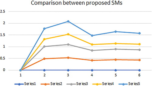
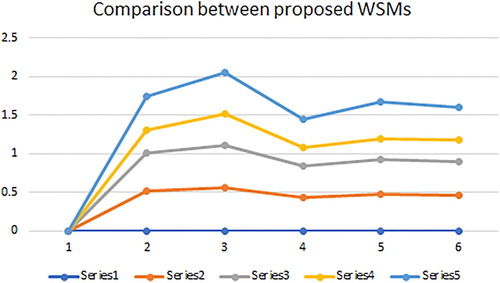
The ranking of the proposed SMs and WSMs are also stated in Tables 1 and 2 respectively. The graphical representation of the proposed SMs is shown in Figure 1 and proposed WSMs are shown in Figure 2.

Figure 2. Graphical representation of established SMs for Example 3.

5.2. Medical Diagnosis

The symptoms of different diseases are different. The medical diagnosis depends on the victim’s symptoms which show what type of disease a victim has. The multiple symptoms of a victim represent a symptom set and a set of diseases can represent by different diseases.

Example 4:

Let a set of diagnoses $\mathcal{D}=\left\{{\mathcal{D}}_1\left(Coronovirous\right),{\mathcal{D}}_2\left(Pneumonia\right),{\mathcal{D}}_3\left(Flu\right),{\mathcal{D}}_4\right.\left.\left(Chestproblem\right)\right\}$ and a set of symptoms $X=\left\{x_1\right(shortofbreath),x_2(Fever),x_3(cough),x_4(chestpain\left)\right\}$. The victim’s symptoms can be showed in the form of CHFSs as below $\mathcal{P}=\left\{\begin{array}{c}\left(x_1,\left\{0.9e^{i2\pi \left(1\right)},0.5e^{i2\pi \left(1\right)},0.5e^{i2\pi \left(0.5\right)}\right\}\right),\left(x_2,\left\{0.5e^{i2\pi \left(0.8\right)},0.7e^{i2\pi \left(0.3\right)},0.4e^{i2\pi \left(0.4\right)}\right\}\right),\\ \left(x_3,\left\{0.2e^{i2\pi \left(0.6\right)},0.8e^{i2\pi \left(0.9\right)}\right\}\right),\left(x_4,\left\{0.1e^{i2\pi \left(0.3\right)}\right\}\right)\end{array}\right\}$ The symptoms of each disease ${\mathcal{D}}_j\left(j=1,2,3,4\right)$ can be showed in CHFSs as below ${\mathcal{D}}_1\left(coronovirous\right)=\left\{\begin{array}{c}\left(x_1,\left\{1e^{i2\pi \left(0.5\right)},0.8e^{i2\pi \left(0.8\right)}\right\}\right),\left(x_2,\left\{0.5e^{i2\pi \left(0.7\right)},0.6e^{i2\pi \left(0.9\right)}\right\}\right),\\ \left(x_3,\left\{0.8e^{i2\pi \left(0.7\right)},0.6e^{i2\pi \left(1\right)},0.9e^{i2\pi \left(0.7\right)}\right\}\right),\left(x_4,\left\{0.1e^{i2\pi \left(0.1\right)}\right\}\right),\end{array}\right\}$ ${\mathcal{D}}_2\left(Pneumonia\right)=\left\{\begin{array}{c}\left(x_1,\left\{0.1e^{i2\pi \left(0.2\right)}\right\}\right),\left(x_2,\left\{0.6e^{i2\pi \left(0.7\right)},0.4e^{i2\pi \left(0.9\right)}\right\}\right),\\ \left(x_3,\left\{0.4e^{i2\pi \left(0.6\right)},0.5e^{i2\pi \left(0.6\right)}\right\}\right),\left(x_4,\left\{0.3e^{i2\pi \left(0.4\right)},0.4e^{i2\pi \left(0.2\right)}\right\}\right)\end{array}\right\}$ ${\mathcal{D}}_3\left(Flu\right)=\left\{\begin{array}{c}\left(x_1,\left\{0.1e^{i2\pi \left(0.0\right)}\right\}\right),\left(x_2,\left\{0.3e^{i2\pi \left(0.2\right)},0.2e^{i2\pi \left(0.5\right)}\right\}\right),\\ \left(x_3,\left\{1e^{i2\pi \left(0.8\right)},0.6e^{i2\pi \left(0.7\right)},0.9e^{i2\pi \left(0.6\right)}\right\}\right),\left(x_4,\left\{0.1e^{i2\pi \left(0.2\right)},0.2e^{i2\pi \left(0.4\right)}\right\}\right)\end{array}\right\}$ ${\mathcal{D}}_4\left(Chestpain\right)=\left\{\begin{array}{c}\left(x_1,\left\{0.2e^{i2\pi \left(0.1\right)},0.3e^{i2\pi \left(0.2\right)}\right\}\right),\left(x_2,\left\{\mathrm{0.1.}{e}^{i2\pi \left(0.2\right)},0.0e^{i2\pi \left(0.2\right)}\right\}\right),\\ \left(x_3,\left\{0.1e^{i2\pi \left(0.3\right)}\right\}\right),\left(x_4,\left\{1e^{i2\pi \left(0.9\right)},0.9e^{i2\pi \left(0.7\right)},0.5e^{i2\pi \left(0.6\right)}\right\}\right)\end{array}\right\}$

In Table 3 we calculated the proposed SMs from $\mathcal{P}$ to ${\mathcal{D}}_j\left(j=1,2,3,4\right)$. The motive of this issue is to know about the disease of the victim that what disease a victim has in the above four diseases ${\mathcal{D}}_j\left(j=1,2,3,4\right)$. From the calculation stated in Table 3, we obtained that the similarity degree between $\mathcal{P}$ and ${\mathcal{D}}_1$ is a massive one as got by all SMs. So by the principle of the maximum degree of similarity, we can say that a victim has coronavirus.

Table 3. Calculation of proposed SMs for $\lambda =1$ and $\left({\alpha }_{cc},{\text{β}}_{cc}\right)=\left(0.5,0.5\right)$.

Similarity measures	${\mathcal{D}}_1$	${\mathcal{D}}_2$	${\mathcal{D}}_3$	${\mathcal{D}}_4$	Ranking
$S_c^1\left(\mathcal{P},{\mathcal{D}}_j\right)$	0.5396	0.5083	0.4023	0.2781	${\mathcal{D}}_1\ge {\mathcal{D}}_2\ge {\mathcal{D}}_3\ge {\mathcal{D}}_4$
$S_c^2\left(\mathcal{P},{\mathcal{D}}_j\right)$	0.6447	0.5759	0.4881	0.3554	${\mathcal{D}}_1\ge {\mathcal{D}}_2\ge {\mathcal{D}}_3\ge {\mathcal{D}}_4$
$S_c^3\left(\mathcal{P},{\mathcal{D}}_j\right)$	0.4588	0.4335	0.336	0.2173	${\mathcal{D}}_1\ge {\mathcal{D}}_2\ge {\mathcal{D}}_3\ge {\mathcal{D}}_4$
$S_c^4\left(\mathcal{P},{\mathcal{D}}_j\right)$	0.5249	0.3981	0.2614	0.1474	${\mathcal{D}}_1\ge {\mathcal{D}}_2\ge {\mathcal{D}}_3\ge {\mathcal{D}}_4$
$S_c^5\left(\mathcal{P},{\mathcal{D}}_j\right)$	0.5713	0.3956	0.2675	0.1488	${\mathcal{D}}_1\ge {\mathcal{D}}_2\ge {\mathcal{D}}_3\ge {\mathcal{D}}_4$

If we let the weight of each element $x_k\left(k=1,2,3,4\right)$ are $0.1,0.2,0.3$ and $0.4$ respectively. Then the calculation of proposed SMs are stated in Table 4. From the calculation stated in Table 4, we obtained the following consequences

1. The similarity degree between $\mathcal{P}$ and ${\mathcal{D}}_1$ is a massive one as got by SMs, ${\text{SM}}_{c_w}^2$, ${\text{SM}}_{c_w}^4$, and ${\text{SM}}_{c_w}^5$. So by the principle of the maximum degree of similarity the SMs ${\text{SM}}_{c_w}^2$, ${\text{SM}}_{c_w}^4$ and ${\text{SM}}_{c_w}^5$ give us that a victim has coronavirus.

2. The similarity degree between $\mathcal{P}$ and ${\mathcal{D}}_2$ is a massive one as got by SMs, ${\text{SM}}_{c_w}^1$, and ${\text{SM}}_{c_w}^3$. So by the principle of the maximum degree of similarity the SMs ${\text{SM}}_{c_w}^1$, and ${\text{SM}}_{c_w}^3$ provide that a victim has pneumonia.

Table 4. Calculation of proposed WSMs for Example (4) based on $\lambda =1$ and $\left({\alpha }_{cc},{\text{β}}_{cc}\right)=\left(0.5,0.5\right)$.

Similarity measures	${\mathcal{D}}_1$	${\mathcal{D}}_2$	${\mathcal{D}}_3$	${\mathcal{D}}_4$	Ranking
$S_{c_w}^1\left(\mathcal{P},{\mathcal{D}}_j\right)$	0.5633	0.5821	0.4749	0.2692	${\mathcal{D}}_2\ge {\mathcal{D}}_1\ge {\mathcal{D}}_3\ge {\mathcal{D}}_4$
$S_{c_w}^2\left(\mathcal{P},{\mathcal{D}}_j\right)$	0.6802	0.6525	0.5662	0.3376	${\mathcal{D}}_1\ge {\mathcal{D}}_2\ge {\mathcal{D}}_3\ge {\mathcal{D}}_4$
$S_{c_w}^3\left(\mathcal{P},{\mathcal{D}}_j\right)$	0.4852	0.5013	0.4022	0.2099	${\mathcal{D}}_2\ge {\mathcal{D}}_1\ge {\mathcal{D}}_3\ge {\mathcal{D}}_4$
$S_{c_w}^4\left(\mathcal{P},{\mathcal{D}}_j\right)$	0.5106	0.4423	0.3089	0.1332	${\mathcal{D}}_1\ge {\mathcal{D}}_2\ge {\mathcal{D}}_3\ge {\mathcal{D}}_4$
$S_{c_w}^5\left(\mathcal{P},{\mathcal{D}}_j\right)$	0.5812	0.4433	0.3163	0.1327	${\mathcal{D}}_1\ge {\mathcal{D}}_2\ge {\mathcal{D}}_3\ge {\mathcal{D}}_4$

The ranking of the proposed SMs and WSMs are also stated in Tables 3 and 4 respectively. The graphical representation of the proposed SMs is shown in Figure 2 and proposed WSMs are shown in Figure 3.

Figure 3. Graphical representation of established WSMs for Example 3.

6. Comparison

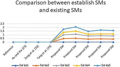
Our goal to expand the new SMs is to deal with new kinds of data such as CHFSs and existing data CFSs, HFSs, and FSs. In this portion, we expressed the benefits of proposed SMs by comparing with existing SMs. The geometrical representations of the information's of example 4 and example 5, are discussed in Figures 4–7.

Figure 4. Graphical representation of established WSMs for Example 4.

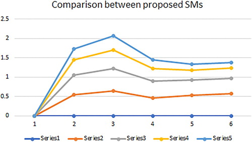
Figure 5. Graphical representation of established WSMs for Example 4.

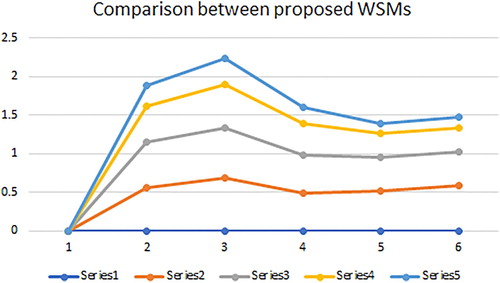
Figure 6. Graphical representation of the comparison of the establish SMs with existing SMs for Example 5.

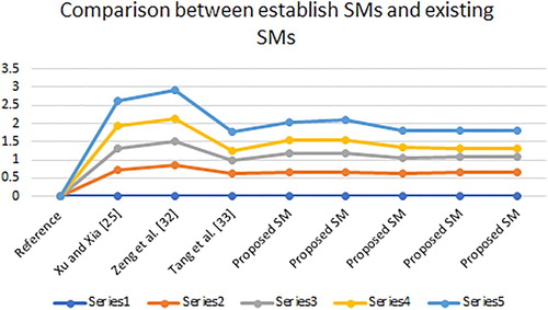
Figure 7. Graphical representation of the comparison of the establish SMs with existing SMs for Example 3.

Example 5:

Let $X=\left\{x_1,x_2,x_3,x_4\right\}$ be a set and four know patterns $E_j\left(j=1,2,3,4\right)$ which are given in the form of HFSs as follows $E_1=\left\{\begin{array}{c}\left(x_1,\left\{0.1,0.4,0.6\right\}\right),\left(x_2,\left\{0.4,1\right\}\right),\\ \left(x_3,\left\{0.7,0.8\right\}\right),\left(x_4,\left\{0.2\right\}\right),\end{array}\right\}$ $E_2=\left\{\begin{array}{c}\left(x_1,\left\{0.3,0.5,0.8\right\}\right),\left(x_2,\left\{\mathrm{0.4.},0.6\right\}\right),\\ \left(x_3,\left\{0.1,0.3\right\}\right),\left(x_4,\left\{0.2,0.4,0.7\right\}\right)\end{array}\right\}$ $E_3=\left\{\begin{array}{c}\left(x_1,\left\{0.6,0.8\right\}\right),\left(x_2,0.1,0.2,0.6\right),\\ \left(x_3,\left\{0.7\right\}\right),\left(x_4,\left\{0.4,0.5\right\}\right)\end{array}\right\}$ $E_4=\left\{\begin{array}{c}\left(x_1,\left\{0.1,0.3\right\}\right),\left(x_2,\left\{0.4,0.8\right\}\right),\\ \left(x_3,\left\{0.4,0.7,0.8\right\}\right),\left(x_4,\left\{0.4\right\}\right),\end{array}\right\}$

Next let an unknown pattern which need to be identify $E=\left\{\begin{array}{c}\left(x_1,\left\{0.2,0.3,0.6\right\}\right),\left(x_2,\left\{0.8,1\right\}\right),\\ \left(x_3,\left\{0.5,0.8\right\}\right),\left(x_4,\left\{1\right\}\right)\end{array}\right\}$

Now we have that $e^0=1$ then the data given in the HFSs converted into the CHFSs as follows $E_1=\left\{\begin{array}{c}\left(x_1,\left\{0.1e^{i2\pi \left(0.0\right)},0.4e^{i2\pi \left(0.0\right)},0.6e^{i2\pi \left(0.0\right)}\right\}\right),\left(x_2,\left\{0.4e^{i2\pi \left(0.0\right)},0.1e^{i2\pi \left(0.0\right)}\right\}\right),\\ \left(x_3,\left\{0.7e^{i2\pi \left(0.0\right)},0.8e^{i2\pi \left(0.0\right)}\right\}\right),\left(x_4,\left\{\mathrm{0.2.}{e}^{i2\pi \left(0.0\right)}\right\}\right)\end{array}\right\}$ $E_2=\left\{\begin{array}{c}\left(x_1,\left\{0.3e^{i2\pi \left(0.0\right)},0.5e^{i2\pi \left(0.0\right)},0.8e^{i2\pi \left(0.0\right)}\right\}\right),\left(x_2,\left\{0.4e^{i2\pi \left(0.0\right)},\mathrm{0.6.}{e}^{i2\pi \left(0.0\right)}\right\}\right),\\ \left(x_3,\left\{0.1e^{i2\pi \left(0.0\right)},0.3e^{i2\pi \left(0.0\right)}\right\}\right),\left(x_4,\left\{0.2e^{i2\pi \left(0.0\right)},0.4e^{i2\pi \left(0.0\right)},0.7e^{i2\pi \left(0.0\right)}\right\}\right)\end{array}\right\}$ $E_3=\left\{\begin{array}{c}\left(x_1,\left\{0.6e^{i2\pi \left(0.0\right)},0.8e^{i2\pi \left(0.0\right)}\right\}\right),\left(x_2,\left\{0.1e^{i2\pi \left(0.0\right)},0.2e^{i2\pi \left(0.0\right)},0.6e^{i2\pi \left(0.0\right)}\right\}\right),\\ \left(x_3,\left\{0.7e^{i2\pi \left(0.0\right)}\right\}\right),\left(x_4,\left\{0.4e^{i2\pi \left(0.0\right)},0.5e^{i2\pi \left(0.0\right)}\right\}\right)\end{array}\right\}$ $E_4=\left\{\begin{array}{c}\left(x_1,\left\{\mathrm{0.9.}{e}^{i2\pi \left(0.0\right)},1.e^{i2\pi \left(0.0\right)},1.e^{i2\pi \left(0.0\right)}\right\}\right),\left(x_2,\left\{\mathrm{0.1.}{e}^{i2\pi \left(0.0\right)},\mathrm{0.3.}{e}^{i2\pi \left(0.0\right)}\right\}\right),\\ \left(x_3,\left\{0.4e^{i\pi \left(0.0\right)},0.7e^{i2\pi \left(0.0\right)},0.8e^{i2\pi \left(0.0\right)}\right\}\right),\left(x_4,\left\{0.4e^{i2\pi \left(0.0\right)}\right\}\right)\end{array}\right\}$

And $E=\left\{\begin{array}{c}\left(x_1,\left\{0.2e^{i2\pi \left(0.0\right)},0.3e^{i2\pi \left(0.0\right)},0.6e^{i2\pi \left(0.0\right)}\right\}\right),\left(x_2,\left\{0.8e^{i2\pi \left(0.0\right)},1e^{i2\pi \left(0.0\right)}\right\}\right),\\ \left(x_3,\left\{0.5e^{i2\pi \left(0.0\right)},0.8e^{i2\pi \left(0.0\right)}\right\}\right),\left(x_4,\left\{1e^{i2\pi \left(0.0\right)}\right\}\right)\end{array}\right\}$

From Table 5 we can observe that the data in the form of FSs and HFSs are solvable through existing SMs in the literature. The data in Example 5 is in the form HFSs which we can convert to CHFSs by taking $1=e^0$ and through proposed SMs we get the similarity between $E$ and $E_j\left(j=1,2,3,4\right)$ as shown in Table 5. But what about the data in the form of CFSs and CHFSs, these type of data are unsolvable through the existing SMs as shown in Table 6. The data in Example 3 are in the form of CHFSs so we can find the similarity between $E$ and $E_j\left(j=1,2,3,4\right)$ through proposed SMs. This means that our proposed SMs are the extension of the existing SMs. Through the proposed SMs we can find the similarity between FS, HFS, CFS, and CHFSs. The ranking of Example 5 is given in Table 5. The similarity degree between $E$ and $E_1$ is a massive one as got by all SMs in Example 5. The ranking of Example 3 given in Table 6 is slightly different than ranking given in Table 5. The similarity degree between $E$ and $E_2$ is a massive one as got by SMs, ${\text{SM}}_c^1$, ${\text{SM}}_c^2$, and ${\text{SM}}_c^3$ and the similarity degree between $E$ and $E_4$ is a massive one as got by SMs, ${\text{SM}}_c^4$ and ${\text{SM}}_c^5$.

Table 5. Comparison between Proposed SMs and Existing SMs for Example (5) and $\lambda =1$, $\left({\alpha }_{cc},{\text{β}}_{cc}\right)=\left(1,0\right)$.

Method	Score value	Ranking
Xu and Xia [25]	$s_g\left(E,E_1\right)=$0.7083, $s_g\left(E,E_2\right)=0.6042$ $s_g\left(E,E_3\right)=0.6083$, $s_g\left(E,E_4\right)=0.7$	$E_1\ge E_4\ge E_3\ge E_2$
Zeng et al. [32]	$s_h\left(E,E_1\right)=0.8375$, $s_h\left(E,E_2\right)=0.6792$ $s_h\left(E,E_3\right)=0.6167$, $s_h\left(E,E_4\right)=0.7979$	$E_1\ge E_4\ge E_2\ge E_3$
Tang et al. [33]	$s_h^{\mathrm{\prime }}\left(E,E_1\right)=0.6319$, $s_h^{\mathrm{\prime }}\left(E,E_2\right)=0.3652$ $s_h^{\mathrm{\prime }}\left(E,E_3\right)=0.2333,$ $s_h^{\mathrm{\prime }}\left(E,E_4\right)=0.5541$	$E_1\ge E_4\ge E_2\ge E_3$
Proposed SM	$S_c^1\left(E,E_1\right)=$0.6664, $S_c^1\left(E,E_2\right)=0.5127$ $S_c^1\left(E,E_3\right)=$0.3563, $S_c^1\left(E,E_4\right)=0.4819$	$E_1\ge E_4\ge E_2\ge E_3$
Proposed SM	$S_c^2\left(E,E_1\right)=0.6664$, $S_c^2\left(E,E_2\right)=$0.5127 $S_c^2\left(E,E_4\right)=0.3563$, $S_c^2\left(E,E_5\right)=0.5582$	$E_1\ge E_4\ge E_2\ge E_3$
Proposed SM	$S_c^3\left(E,E_1\right)=0.6177$, $S_c^3\left(E,E_2\right)=0.4366$ $S_c^3\left(E,E_3\right)=0.2833$, $S_c^3\left(E,E_4\right)=0.4775$	$E_1\ge E_4\ge E_2\ge E_3$
Proposed SM	$S_c^4\left(E,E_1\right)=0.6694$, $S_c^4\left(E,E_2\right)=0.4115$ $S_c^4\left(E,E_3\right)=0.2438$, $S_c^4\left(E,E_4\right)=0.4885$	$E_1\ge E_4\ge E_2\ge E_3$
Proposed SM	$S_c^5\left(E,E_1\right)=0.6694$, $S_c^5\left(E,E_2\right)=0.4115$ $S_c^5\left(E,E_3\right)=0.2438$, $S_c^5\left(E,E_4\right)=0.4885$	$E_1\ge E_4\ge E_2\ge E_3$

Table 6. Comparison between proposed SMs with existing SMs for Example (3) and $\lambda =1$.

Method	Score value	Ranking
Xu and Xia [25]	Failed	Failed
Zeng et al. [32]	Failed	Failed
Tang et al. [33]	Failed	Failed
Proposed SM	$S_c^1\left(E,E_1\right)=0.4928$,$S_c^1\left(E,E_2\right)=$0.5109 $S_c^1\left(E,E_3\right)=0.3218$, $S_c^1\left(E,E_4\right)=0.4503$	$E_2\ge E_1\ge E_4\ge E_3$
Proposed SM	$S_c^2\left(E,E_1\right)=0.5316$,$S_c^2\left(E,E_2\right)=0.5686$ $S_c^2\left(E,E_3\right)=0.4309$, $S_c^2\left(E,E_4\right)=0.555$	$E_2\ge E_4\ge E_1\ge E_3$
Proposed SM	$S_c^3\left(E,E_1\right)=0.4175$,$S_c^3\left(E,E_2\right)=0.4281$ $S_c^3\left(E,E_3\right)=0.2536$, $S_c^3\left(E,E_4\right)=0.3801$	$E_2\ge E_4\ge E_1\ge E_3$
Proposed SM	$S_c^4\left(E,E_1\right)=0.4465$,$S_c^4\left(E,E_2\right)=0.4448$ $S_c^4\left(E,E_3\right)=0.2529$, $S_c^4\left(E,E_4\right)=0.5003$	$E_4\ge E_2\ge E_1\ge E_3$
Proposed SM	$S_c^5\left(E,E_1\right)=0.4366$,$S_c^5\left(E,E_2\right)=0.4259$ $S_c^5\left(E,E_3\right)=0.2516$, $S_c^5\left(E,E_4\right)=0.4667$	$E_4\ge E_1\ge E_2\ge E_3$

7. Conclusion

SMs are utilized to inspect the variation between the two objects. The purpose of this article is to define the fundamental notion of CHFSs which is the combination of HFS and CFS and also defined their fundamental properties. We explored SMs for CHFSs. We presented exponential based generalized SMs and without exponential based generalized SMs for CHFSs. We obtained some valuable remarks. Further, the established SMs are used in Pattern recognition and medical diagnosis to inspect the practicability and credibility of the established SMs. Furthermore, we solved numerical examples for established SMs to show the supremacy and integrity of the proposed SMs. At last, to assess the trustworthiness of the established SMs we represented the comparison of the established SMs with some existing SMs. Our future work is to explore the application of CHFNs in many other type of researches [34–48].

Disclosure statement

No potential conflict of interest was reported by the authors.

Additional information

Notes on contributors

Tahir Mahmood

Tahir Mahmood is Assistant Professor of Mathematics at Department of Mathematics and Statistics, International Islamic University Islamabad, Pakistan. He received his Ph.D. degree in Mathematics from Quaid-i-Azam University Islamabad, Pakistan in 2012 under the supervision of Professor Dr. Muhammad Shabir. His areas of interest are Algebraic structures, Fuzzy Algebraic structures and Soft sets. He has more than 65 international publications to his credit and he has also produced 38 MS students.

Ubaid ur Rehman

Ubaid ur Rehman, received the M.Sc. degrees in Mathematics from International Islamic University Islamabad, in 2018. Currently, He is a Student of MS in mathematics from International Islamic University Islamabad, Pakistan. His research interests include similarity measures, distance measures, fuzzy logic, fuzzy decision making, and their applications.

Zeeshan Ali

Zeeshan Ali, received the B.S. degrees in Mathematics from Abdul Wali Khan University Mardan, Pakistan, in 2016. He received has M.S. degrees in Mathematics from International Islamic University Islamabad, Pakistan, in 2018. Currently, He is a Student of Ph.D. in mathematics from International Islamic University Islamabad, Pakistan. His research interests include aggregation operators, fuzzy logic, fuzzy decision making, and their applications. He has published more than Thirteen articles.

References

- Zadeh LA. Fuzzy sets. Inf Control. 1965;8(3):338–353.
- Adlassnig KP. Fuzzy set theory in medical diagnosis. IEEE Trans Sys Man Cybe. 1986;16(2):260–265.
- Chen SM. A weighted fuzzy reasoning algorithm for medical diagnosis. Decis Support Syst. 1994;11(1):37–43.
- Smets P. Medical diagnosis: fuzzy sets and degrees of belief. Fuzzy Sets Syst. 1981;5(3):259–266.
- Mitra S, Pal SK. Fuzzy sets in pattern recognition and machine intelligence. Fuzzy Sets Syst. 2005;156(3):381–386.
- Yager RR. Multiple objective decision-making using fuzzy sets. Int J Man Mach Stud. 1977;9(4):375–382.
- Zadeh LA. The Concept of a Linguistic Variable and its Application to Approximate Reasoning. In: Fu KS, Tou JT (eds). Learning Systems and Intelligent Robots. Boston (MA): Springer; 1974. p. 1–10.
- Couso I, Garrido L, SáNchez L. Similarity and dissimilarity measures between fuzzy sets: a formal relational study. Inf Sci (Ny). 2013;229:122–141.
- Lee-Kwang H, Song YS, Lee KM. Similarity measure between fuzzy sets and between elements. Fuzzy Sets Syst. 1994;62(3):291–293.
- Pramanik S, Mondal K. Weighted fuzzy similarity measure based on tangent function and its application to medical diagnosis. Infinite Study. 2015;4:158–164.
- Wang WJ. New similarity measures on fuzzy sets and on elements. Fuzzy Sets Syst. 1997;85(3):305–309.
- Kwon SH. A similarity measure of fuzzy sets. J Korean Instit Intell Sys. 2001;11(3):270–274.
- Guha D, Chakraborty D. A new approach to fuzzy distance measure and similarity measure between two generalized fuzzy numbers. Appl Soft Comput. 2010;10(1):90–99.
- Kakati PP. A note on the new similarity measure for fuzzy sets. Int J Comp Appl Tech Res. 2013;2(5):601–605.
- Hesamian G. Fuzzy similarity measure based on fuzzy sets. Control Cybern. 2017;46(1):71–86.
- Ramot D, Milo R, Friedman M, et al. Complex fuzzy sets. IEEE Trans Fuzzy Syst. 2002;10(2):171–186.
- Bi L, Dai S, Hu B, et al. Complex fuzzy arithmetic aggregation operators. J Intell Fuzzy Syst. 2019;36(3):2765–2771.
- Li C. Adaptive image restoration by a novel neuro-fuzzy approach using complex fuzzy sets. Int J Intell Inf Database Syst. 2013;7(6):479–495.
- Yazdanbakhsh O, Dick S. A systematic review of complex fuzzy sets and logic. Fuzzy Sets Syst. 2018;338:1–22.
- Dai S. Comment on “toward complex fuzzy logic”. IEEE Trans Fuzzy Syst. 2019;1–1.
- Jun YB, Xin XL. Complex fuzzy sets with application in BCK/BCI-Algebras. Bull Sec Logic. 2019;48(3):173–185.
- Hu B, Bi L, Dai S. The orthogonality between complex fuzzy sets and its application to signal detection. Symmetry (Basel). 2017;9(9):175.
- Hu B, Bi L, Dai S, et al. Distances of complex fuzzy sets and continuity of complex fuzzy operations. J Intell Fuzzy Syst. 2018;35(2):2247–2255.
- Torra V. Hesitant fuzzy sets. Int J Intell Syst. 2010;25(6):529–539.
- Xu Z, Xia M. Distance and similarity measures for hesitant fuzzy sets. Inf Sci (Ny). 2011;181(11):2128–2138.
- Liao H, Xu Z. Subtraction and division operations over hesitant fuzzy sets. J Intell Fuzzy Syst. 2014;27(1):65–72.
- Alcantud JCR, Torra V. Decomposition theorems and extension principles for hesitant fuzzy sets. Inf Fusion. 2018;41:48–56.
- Bisht K, Kumar S. Fuzzy time series forecasting method based on hesitant fuzzy sets. Expert Syst Appl. 2016;64:557–568.
- Zhang X, Xu Z. Novel distance and similarity measures on hesitant fuzzy sets with applications to clustering analysis. J Intell Fuzzy Syst. 2015;28(5):2279–2296.
- Alcantud JCR, Giarlotta A. Necessary and possible hesitant fuzzy sets: a novel model for group decision making. Inf Fusion. 2019;46:63–76.
- Farhadinia B, Herrera-Viedma E. Multiple criteria group decision making method based on extended hesitant fuzzy sets with unknown weight information. Appl Soft Comput. 2019;78:310–323.
- Zeng W, Li D, Yin Q. Distance and similarity measures between hesitant fuzzy sets and their application in pattern recognition. Pattern Recognit Lett. 2016;84:267–271.
- Tang X, Peng Z, Ding H, et al. Novel distance and similarity measures for hesitant fuzzy sets and their applications to multiple attribute decision making. J Intell Fuzzy Syst. 2018;34(6):3903–3916.
- Liu P, Mahmood T, Ali Z. Complex q-Rung Orthopair fuzzy aggregation operators and their applications in multi-attribute group decision making. Information. 2020;11(1):5.
- Liu P, Ali Z, Mahmood T. A method to multi-attribute group decision-making problem with complex q-Rung Orthopair linguistic information based on Heronian mean operators. Int J Comp Intell Sys. 2019;12(2):1465–1496.
- Ullah K, Mahmood T, Ali Z, et al. On some distance measures of complex Pythagorean fuzzy sets and their applications in pattern recognition. Compl Intell Sys. 2019;6:1–13.
- Ullah K, Garg H, Mahmood T, et al. Correlation coefficients for T-spherical fuzzy sets and their applications in clustering and multi-attribute decision making. Soft Comput. 2019;24:1–13.
- Ali Z, Mahmood T. Complex neutrosophic generalized dice similarity measures and their application to decision making. CAAI Trans Intell Technol. 2020;5:1–10.
- Jan N, Zedam L, Mahmood T, et al. Multiple attribute decision making method under linguistic cubic information. J Intell Fuz Sys (Preprint). 2019;36:1–17.
- Ullah K, Mahmood T, Jan N, et al. A note on geometric aggregation operators in spherical fuzzy environment and its application in multi-attribute decision making. J Eng Appl Sci. 2018;37(2):75–86.
- Zhang D, Wu C, Liu J. Ranking products with online reviews: a novel method based on hesitant fuzzy set and sentiment word framework. J Oper Res Soc. 2020;71(3):528–542.
- Torra V, Narukawa Y. On hesitant fuzzy sets and decision. In 2009 IEEE International Conference on Fuzzy Systems. IEEE; 2009, Aug. p. 1378–1382.
- Qian G, Wang H, Feng X. Generalized hesitant fuzzy sets and their application in decision support system. Knowl Based Syst. 2013;37:357–365.
- Rodríguez RM, Martínez L, Torra V, et al. Hesitant fuzzy sets: state of the art and future directions. Int J Intell Syst. 2014;29(6):495–524.
- Xu, Z. Hesitant fuzzy sets theory (Vol. 314). Cham: Springer International Publishing; 2014.
- Wei G. Hesitant fuzzy prioritized operators and their application to multiple attribute decision making. Knowl Based Syst. 2012;31:176–182.
- Wang JQ, Wang DD, yu Zhang H, et al. Multi-criteria outranking approach with hesitant fuzzy sets. OR Spectrum. 2014;36(4):1001–1019.
- Faizi S, Rashid T, Sałabun W, et al. Decision making with uncertainty using hesitant fuzzy sets. Int J Fuzzy Syst. 2018;20(1):93–103.