
 ?Mathematical formulae have been encoded as MathML and are displayed in this HTML version using MathJax in order to improve their display. Uncheck the box to turn MathJax off. This feature requires Javascript. Click on a formula to zoom.
Abstract
In this paper, the concept of the -polar fuzzy graph (
-PFG) and interval-valued fuzzy graph (IVFG) is integrated and introduced an unprecedented kind of fuzzy graph designated as
-polar interval-valued fuzzy graph (
-PIVFG). Complement of the
-PIVFG is defined and the failure of this definition in some cases are highlighted. Various examples are cited and then redefined the notation of complement such that it applies to all
-PIVFGs. The other algebraic properties such as isomorphism, weak isomorphism, co-weak isomorphism of the
-PIVFG are investigated. Moreover, some basic results on the isomorphic property of
-PIVFG are proved. Finally, an application of
-PIVFG is explored.
Abbreviations: The following abbreviations are employed in this study: FS: Fuzzy set; FG: Fuzzy graph; IVFS: Interval-valued fuzzy sets; IVFG: Interval-valued fuzzy graph; -PFS:
-polar fuzzy sets;
-PFG:
-polar fuzzy graph;
-PIVFS:
-polar interval-valued fuzzy sets;
-PIVFG:
-polar interval-valued fuzzy graph.
1. Introduction
A graph is a mathematical structure used to represent pairwise relations between objects. It is defined as an ordered pair consisting of a set of vertices, designated as
and a set of edges, denoted by
. When there is a vagueness either in vertices or in edges or in both then a fuzzy model is needed to describe a fuzzy graph. With the Konigsberg bridge problem, the graph theory was started in 1735. The concept was first introduced by Swiss Mathematician Euler in 1736. Then, Euler studied and incorporated a structure that solves the Konigsberg bridge problem which is also known as a Eulerian graph. Thereafter, the complete and bipartite graphs were proposed by Mobius in 1840. Recently, applications of graph theory are mostly promoted to the areas of computer networks, electrical networks, coding theory, operational research, architecture, data mining, etc.
Observing the vast application of graph theory motivated to explain fuzzy graph which is a non-empty set together with a fuzzy set and a fuzzy relation. In 1973, Kauffman [Citation1] defined fuzzy graph depending on the idea of fuzzy set introduced by Zadeh [Citation2]. In 1975, Rosenfeld [Citation3] first proposed another definition of the Fuzzy graph which is a generalization of Euler's Graph theory. He also elaborated definition of fuzzy vertex, fuzzy edges and several fuzzy concepts such as cycles, paths, connectedness, etc. The idea of isomorphism, weak isomorphism, co-weak isomorphism between fuzzy graphs was introduced by Bhutani [Citation4] in 1989. The extension of the concept of fuzzy set and the idea of bipolar fuzzy sets were given in 1994 by Zhang [Citation5, Citation6]. Several properties of fuzzy graphs and hypergraphs were discussed by Mordeson and Nair [Citation7–9] in 2000.
IVFG was defined by Hongmei and Lianhua [Citation10] in 2009 and some operations on this were studied by Akram and Dudek [Citation11] in 2011. Complete fuzzy graph was defined by Hawary [Citation12]. He also studied three new operations on it. Nagoorgani and Malarvizhu [Citation13, Citation14] studied isomorphic properties on fuzzy graphs and also defined the self-complementary fuzzy graphs. The extension of bipolar fuzzy set and the idea of -polar fuzzy sets (
-PFS) were introduced by Chen et al. [Citation15] in 2014. Samanta and Pal [Citation16–19] investigated on fuzzy tolerance graph, fuzzy threshold graph, fuzzy
-competition graphs,
-competition fuzzy graphs and also fuzzy planar graphs. Some properties of isomorphism and complement on IVFG were studied by Talebi and Rashmanlou [Citation20]. Later, Ghorai and Pal [Citation21, Citation22] described various properties on
-PFGs. They examined isomorphic properties on
-PFG. Different types of research on generalized fuzzy graphs were discussed on [Citation23–31]. The main contribution of this study is as follows:
Concept of
-PIVFGs and complement of
The definitions of classic and non-classic
Definition of isomorphic, weak isomorphic and co-weak isomorphic
Results based on isomorphic properties of
A case study based on
The rest of the paper is arranged as follows: Section 1 describes the historical backgrounds of Fuzzy graphs. Section 2 provides some basic ideas of the -PFGs, IVFGs with some examples. In Section 3,
-PIVFG is defined and supported with examples. Complete
-PIVFG and strong
-PIVFG are also investigated with suitable examples. Section 4 provides the definition of a complement of an
-PIVFG. This section is based on a description of the complement of an
-PIVFG and some improvements over this definition. In section 5 various types of isomorphic property of
-PIVFGs are described with examples. Some propositions and theorems related to this property are also discussed. Section 6 provides the application of an
-PIVFG in decision-making problems. Section 7 is based on a summary of this article.
2. Preliminaries
In this part, some definitions related to -PFG are defined and demonstrated with the help of examples. The basic definition of IVFG is also discussed in this part, followed by an example for demonstration.
A fuzzy set is a set whose elements have degrees of membership. Fuzzy sets were introduced by Zadeh [Citation2] in 1965 as an extension of the classical notion of the set. A fuzzy set is a pair
where
is a set and
is a membership function. Throughout this article,
is a crisp graph, and
is a fuzzy graph.
Proof
DEFINITION 2.1
([Citation15]) An -PFS (or a [0,1]m-set) on a set
is a mapping
. The set of all
-PFS on
is denoted by
.
Proof
DEFINITION 2.2
[Citation32] Let be an
-PFS on
. An
-polar fuzzy relation on
is an
-PFS
of
such that
i.e. for each
and
.
Proof
DEFINITION 2.3
[Citation32] An -PFG of a crisp graph
is a pair
where
is an
-PFS in
and
is an
-PFS in
such that for each
;
and
, where
is the smallest element in
.
is called the
-polar fuzzy vertex set of
and
is called the
-polar fuzzy edge set of
.
Proof
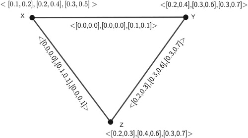
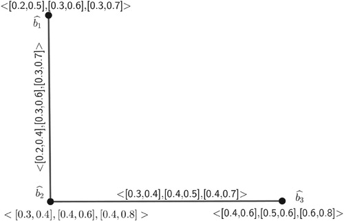
Example 1
The following is an example of an -PFG. Let
be a crisp graph where
and
. Let
be an
-PFS on
and let
be an
-PFS on
defined by Tables and , respectively:
Figure 1. 3-PFG.
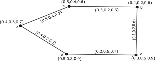
Table 1. -PFS on .
Table 2. -PFS on .
Proof
DEFINITION 2.4
[Citation33] An IVFS on
is defined as
, where
and
are fuzzy subsets on
such that
,
. Based on this set a graph called IVFG is defined.
Proof
DEFINITION 2.5
[Citation10] By an IVFG of a crisp graph we mean
, where
is an IVFS on
and
is an IVFS on
, such that
,
.
Lots of works have been done on this graph [Citation34–38].
Proof
Example 2
The following is an example of IVFG. Let be a crisp graph where
and
. Let A be an IVFS on
and let B be an IVFS on
defined by Tables and , respectively:
In the following section the -PIVFG, a combination of IVFG and
-PFG is defined.
Figure 2. An IVFG.
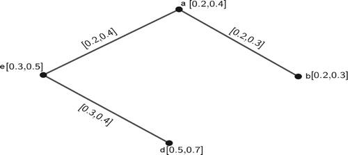
Table 3. IVFS on .
Table 4. IVFS on .
3. -polar Interval-valued Fuzzy Graph (-PIVFG)
Herein, -PFG and IVFG are combined and the concept of
-PIVFG is introduced and demonstrated with examples. Also, in this part we described complete
-PIVFG with appropriate examples and strong
-PIVFG, illustrated with examples.
Proof
DEFINITION 3.1
An -PIVFG of a graph
is a pair
consists of a non-empty set
together with pair of interval-valued function
is an
-PFS in
and
and
for each
;
,
and
,
and for each
, the interval number of vertex
and of the edge
in
respectively satisfying
,
,
.
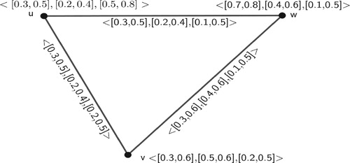
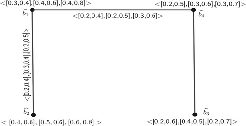
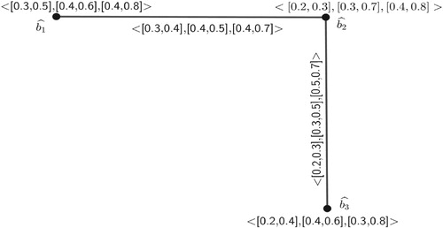
Now, we give an example of -PIVFG:(See ).
Figure 3. A -PIVFG.
Proof
Example 3
Let us consider a -PIVFG
, where
Proof
DEFINITION 3.2
An -PIVFG
of
is said to be complete if
and
for every pair of vertices
and for each
.
Proof
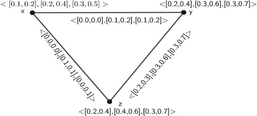
Example 4
Let us consider Example 3, here,
Similarly, we get the edges vw and wu. Hence, the graph G is complete, since for all the pair of vertices
the conditions
and
hold.
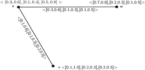
Figure 4. A -PIVFG
which is not complete.
Proof
DEFINITION 3.3
An -PIVFG
of
is said to be strong
-PIVFG if
and
for all the edges
and for each
.
Above described example is an example of a strong -PIVFG. Already, we have discussed that is not complete.
4 Complement of an -PIVFG
In this present section, first, the complement of -PIVFG with suitable examples are defined. Then the limitations of the definitions are observed with the help of some examples. After that new modified definition for the complement is developed and is verified with examples.
Proof
DEFINITION 4.1
Let of
be an
-PIVFG. The complement of
is an
-PIVFG
, where
,
, and
for each
and for every
.
Example 5 The following is an example of an -PIVFG while represents its complement. Let us consider a
-PIVFG
, where
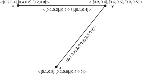
The complement
of
is
Similarly for others, Thus, we get
Construction of complements we just stated by the above definition fails for some
-PIVFG. For further illustration, we consider the examples as follows.
Figure 5. A 3-PIVFG.
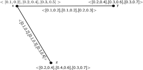
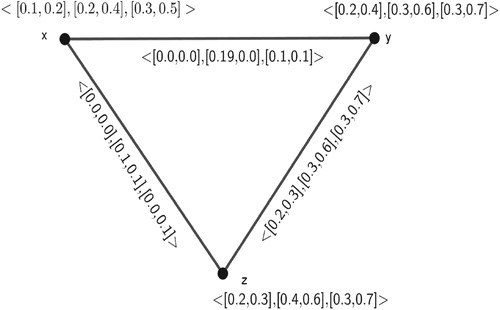
Figure 6. The complement of the 3-PIVFG of .
Example 6 Let us consider a -PIVFG
of
(See ),
The complement
() of
is
Here for i=2, and
,
, which is not an interval. So, we can't construct this type of
-PIVFG.
Figure 7. A 3-PIVFG.
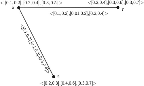
Figure 8. Complement of the 3-PIVFG of .
Keeping in mind the limitations of definition 9 as demonstrated by example 5, we propose a new definition of the complement of -PIVFG which is well defined given below.
Proof
DEFINITION 4.2
Let be an
-PIVFG. Also let
and
represent
and
, respectively. The complement
of
is also an
-PIVFG, where
for each
and for every
.
Example 7 For the above considered -PIVFG
, modified
will be ()
Proof
DEFINITION 4.3
An -PIVFG
of a crisp graph
is called
-PIVFG if all its
-pole of all its edge satisfy the condition
for each
and for every
.
Figure 9. Modified .
Proof
DEFINITION 4.4
Let be an
-PIVFG of a crisp graph
. Then the edge
in
satisfying
, for each
and for every
are called perfect edges and all other edges
for which
, are called imperfect edges
.
Proposition 1:
All the edges of an -PIVFG are perfect iff
-PIVFG is classic.
In the next section, we study various types of isomorphic property of -PIVFG with proper examples. Thereafter, we describe some propositions and theorems of
-PIVFG with the proofs.
5. Isomorphic -PIVFG
Proof
Definition 5.1
Let of
and
of
be two
. A homomorphism
is a mapping
satisfying the following conditions,
1.
2.
Consider a mapping , here,
,
,
,
, and also
,
for
and
. Since all the conditions of homomorphism are hold therefore, there exists a homomorphism
(See Figures and ).
Proof
DEFINITION 5.2
Let of
and
of
be two
-PIVFG. An isomorphism
is a bijective mapping
satisfying the following conditions,
The following -PIVFG depicted in Figures and show that there exists an isomorphism between them by the help of Definition 14.
Figure 10. A -PIVFG
.
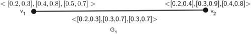
Figure 11. A -PIVFG
.
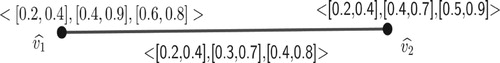
Figure 12. A -PIVFG
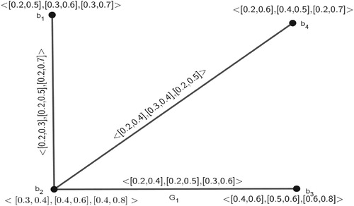
Figure 13. A -PIVFG
.
Example 9 For any two -PIVFG
and
We consider a homomorphism (See Figures and )
where the mapping
satisfies the following criteria,
and
Therefore, there exists an isomorphism
.
Proof
THEOREM 1
Let of
and
of
be two complete
-PIVFGs. Then
is isomorphic to
iff
is isomorphic to
.
Proof.
Let is isomorphic to
, then there exists a bijective mapping
satisfying
Again from the definition of complement for the complete graph,
This implies that
is isomorphic to
. The proof of the converse part is the same as above.
Proof
DEFINITION 5.3
An -PIVFG
is said to be self complementary if
.
Example 10 Let us consider a -PIVFG
described by , where
Complement of
, i.e.
(See ) where
Here, we see
is isomorphic to
. Hence,
is self-complementary.
Figure 14. A -PIVFG
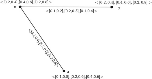
Figure 15. Complement .
Proof
PROPOSITION 2
If is a complete
-PIVFG that is then G is self complementary (Figures and ).
Figure 16. A -PIVFG
.
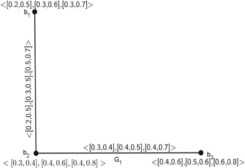
Figure 17. A -PIVFG
.
Proof.
Let be a complete
-PIVFG such that
and
,
.
Now
Similarly, we can prove that
for any
. Therefore,
is self-complementary.
Note 1 Let of
be a strong
-PIVFG. Then
is a strong
-PIVFG if
Proof
THEOREM 2
Let be a strong
-PIVFG of the crisp graph
and
be the complement of
then,
Proof.
Let
If
If for
Proof
THEOREM 3
Let be a self complementary strong
-PIVFG, then for
, and for each
and
.
Proof.
Let be a self-complementary strong
-PIVFG. Then
, for each
,
and
and there exists an isomorphism
such that
Proof
THEOREM 4
Let be a strong
-PIVFG of
. If
and
,
, then
is self-complementary.
Proof.
Let be a strong
-PIVFG, satisfying
and
,
,
, then the identity mapping
is an isomorphism from
to
. Clearly
satisfies the condition of vertices for isomorphism, that is,
and
. And by the Theorem 2,
and
That is,
. Similarly,
,
,
. That imply
satisfies also the condition of edges for isomorphism. Therefore,
. That is
is self-complementary.
Proof
THEOREM 5
Let and
be two strong
-PIVFG. Then
iff
.
Proof.
Assume that and
be two strong
-PIVFG and let us assume
. Then by definition, there exists a bijective mapping
satisfying
Case I: For and for every
. If
… … … … … … … … … … … ..
Case II: If for and
then,
and
. So,
and
and for each
. Hence,
.
Conversely, let , then there exists a bijective mapping
satisfying
Case I: If and for each
,
, then
Again,
. So,
for
.
Case II: If for ,
then,
. Thus,
. Similarly we can prove,
. Hence,
.
Proof
DEFINITION 5.4
Let of
and
of
be two
-PIVFG. A weak isomorphism
is a bijective mapping
satisfying the following conditions,
Example 11 Let us consider any two -PIVFGs
We define a mapping
such that
Since all the conditions satisfied, thus,
is weak-isomorphic to
.
Proof
THEOREM 6
Let us consider a weak isomorphism , then for
, and for each
Proof.
Let us consider a weak isomorphism from
to it's complement
i.e.
. Then
such that
Taking summation both sides,
Similarly we can prove,
. Hence, the result.
Proof
THEOREM 7
Let be an
-PIVFG of
. If
and
,
, then
has a weak isomorphism
from
to it's complement
.
Proof.
Let be an
-PIVFG, satisfying
and
,
,
, then the identity mapping
satisfies the condition
and
and,
and
. That is,
. Similarly,
,
,
. That imply
satisfies also the condition for weak isomorphism from
to it's complement
. Hence,
has a weak isomorphism
from
to it's complement
.
Proof
DEFINITION 5.5
Let of
and
of
be two
-PIVFGs. A co-weak isomorphism
is a bijective mapping
satisfying the following conditions,
Example 12 Let us consider any two -PIVFGs
Here, we define a mapping
like
Thus,
is a co-weak isomorphism (See Figures and ).
Figure 18. A -PIVFG
.
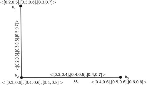
Figure 19. A -PIVFG
Proof
THEOREM 8
Let us consider a co-weak isomorphism , then for
, and for each
Proof.
Let us consider a co-weak isomorphism from
to it's complement
i.e.
. Then
such that
6. Application
Fuzzy graphs have many applications for problems concerning group structures, solving fuzzy intersection equations, etc. An -PFG has applications in decision-making problems including co-operative games, medical diagnosis, signal processing, pattern recognition, robotics, database theory, expert systems and so on. Also,
-PIVFG is used in many decision-making problems. This happens when a democratic country elects its leader, a group of people decide which movie to watch when a company decides which product design to manufacturing, when a group of judges choose a participate in a reality show, etc. Here we consider an example of a singing competition. Let,
be the set of five candidates and
be the set of four judges. They have to select a candidate for the winning trophy depending on their qualities that are voice tone, smoothness, confidence, facial expression, presentation. Suppose Judge ‘a’ is an expert of ‘Sufi music’, judge ‘b’ an expert of ‘Ghazal music’, judge ‘c’ an expert of ‘folk music’ and judge ‘d’ an expert of ‘Indian filmy music’. By default, all the Judges have sufficient knowledge in ‘Classical music’. For each candidate a judge from
can give marks in the form of interval value in [0,1] to
; such as,
Assuming is constructed by the four Judges. The first column represents the performance marks of Aman given by four Judges. Similar to other columns. On the other hand first row represents the marks to all participants given by First Judge. From this table, one can construct a -PIVFG shown in . The first row can be denoted by
, i.e.
. Also,
means a score of the candidate Aman by the judge ‘a’ for the trophy is in between 30 and 60% depending on the qualities Tone, Smoothness, Confidence, Facial expression and Presentation. Similarly for others. Also, an edge represents score by Judges whose fields of music are common. For example Judge ‘a’ who is an expert of ‘Sufi music’ also has ideas on ‘Ghazal music’. Here, the edges
Figure 20. For the graph
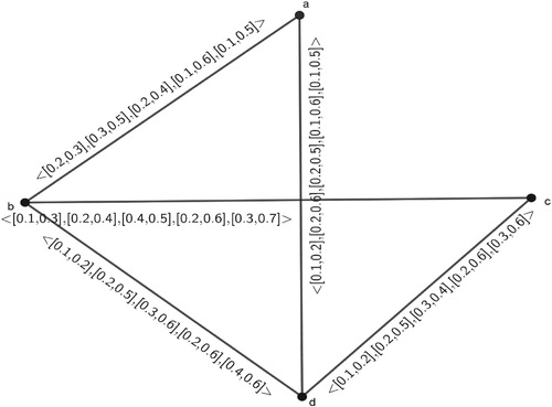
Table 5. Marks given to each candidate.
The judges give marks to the singers by the following rule:
Marks ={(upper limit of the interval + lower limit of the interval)÷2}×100. Marks of each candidate (vi) given by the judges are listed in following table. Then each pair of judges give rank (Ri) to all the candidates (vi) according to their marks (Tables –).
Table 6. Marks given to each candidate.
Table 7. Rank given to each candidate.
Table 8. Score of each candidate.
Depending on the performance of the competitions, each pair of judges prepared a panel for the candidates. Again, to find the combined rank of each candidate based on the rank of all judges we consider weights for a different rank. Suppose be the weights for the rank i. Obviously
for
. Thus the combined rank or say a score of a candidate is given by the formula
. Using this formula the score (sj) of all five candidates are calculated below:
Hence according to the final score, Bibhu get the first position, Karan gets the second position, Piu gets the third position, Survi gets the fourth position and Aman gets the fifth position. The determination of which singer to win the trophy is called the decision-making problem. Moreover, -PIVFG has applications in different areas of computer science, neural intelligence, astronomy, autonomous system and industrial field and so on.
7. Conclusion and Future Research Direction
We have been seen that IVFG being viewed as a generalization of fuzzy graph and -PFG also viewed as an extension of bi-polar fuzzy graph. In this study, we have been introduced the
-PIVFG, a generalization of IVFG and
-PFG, and its complements with examples. The definition of complement has been failed in some cases. Therefore, we have been modified the definition with examples. The definitions of homomorphism, isomorphism, weak isomorphism, co-weak isomorphism of
-PIVFG have been defined with proper given examples. Furthermore, we have been stated the complete
-PIVFG and strong
-PIVFG. In fact, some properties related to complements of complete
-PIVFG and strong
-PIVFG have been described. Thereafter, we also have been discussed few properties regarding self-complementary of
-PIVFG.
We should feature that regarding this investigation, there are distinctive developing regions that we need not demonstrate here as they are outside of our feasible region. In any case, there can be interesting points for future research; for example, one may examine the -PIVFG with various kinds of environments [Citation39], e.g. domination, Pythagorean, fuzzy soft graph [Citation40–44], etc. In the future, we shall investigate other results of
-PIVFG and extend them to solve various problems of decision-making problems under different fuzzy environments.
Disclosure Statement
No potential conflict of interest was reported by the author(s).
Additional information
Notes on contributors
Sanchari Bera
Sanchari Bera is a Research Scholar in the Department of Applied Mathematics with Oceanology and Computer Programming, Vidyasagar University, Midnapore-721102, West Bengal, India. She received her B.Sc (Hons.) and M. Sc. degrees in Mathematics from Raja Narendra Lal Khan Women's College (Autonomous) and Vidyasagar University, West Bengal, India in 2012 and 2014, respectively. Her main research interests include Graph Theory and Fuzzy Graph Theory. She has published two research papers in reputed journals.
Madhumangal Pal
Madhumangal Pal is currently a Professor of Applied Mathematics, Vidyasagar University. He has received Gold and Silver medals from Vidyasagar University for rank first and second in M.Sc. and B.Sc. examinations respectively. Also, he received ‘Computer Division Medal’ from Institute of Engineers (India) in 1996 for best research work. In 2013, he has received Bharat Jyoti Award for the significant contribution in academic. Prof. Pal has successfully guided 34 research scholars for Ph.D. degrees and has published more than 320 articles in international and national journals. His specializations include Algorithmic and Fuzzy Graph Theory, Fuzzy Matrices, Genetic Algorithms and Parallel Algorithms. Prof. Pal is the author of eight text books published from India and United Kingdom and two edited book published by IGI Global, USA. He has published 21 book chapters in several edited books. Prof. Pal completed three research project funded by UGC and DST and one project is going on. Prof. Pal is the Editor-in-Chief of Journal of Physical Sciences', ‘Annals of Pure and Applied Mathematics’, area editor of ‘International Journal of Computational Intelligence Systems (SCI Indexed Journal)’ and member of the editorial Boards of many journals. Also, he has visited China, Greece, London, Taiwan, Malaysia, Thailand, Hong Kong, Dubai and Bangladesh to participated, delivered invited talks and to chair conference event. He is also a member of the American Mathematical Society, USA, Calcutta Mathematical Society, Advanced Discrete Mathematics and Application, Neutrosophic Science International Association, USA, etc. As per Google Scholar, the citation of Prof. Pal is 6233, h-index is 40 and i10-index is 184, as on 25.06.2020. He is the member of several administrative and academic bodies in Vidyasagar University and other institutes/organizations.
References
- Kaufmann A. (1973). Introduction a la Theorie des Sous-emsembles Flous, Masson et cie, Vol.1.
- Zadeh LA. Fuzzy sets. Inf Control. 1965;8:338–353.
- Rosenfield A. Fuzzy graphs, Fuzzy sets and their application (L.A. Zadeh, K.S. Fu,M. Shimura,Eds.): 77–95. New York: Academic press; 1975.
- Bhutani KR. On automorphism of fuzzy graphs. Pattern Recognit Lett. 1989;9(3):159–162.
- Zhang WR. Bipolar fuzzy sets and relations: A computational framework for cognitive modeling and multiagent decision analysis. NAFIPS/IFIS/NASA '94. Proceedings of the First International Joint Conference of The North American Fuzzy Information Processing Society Biannual Conference. The Industrial Fuzzy Control and Intellige; 1994 Dec 18–21; San Antonio, TX, USA. IEEE. p. 305–309.
- Zhang WR. Bipolar fuzzy sets. IEEE Int Conf Fuzzy Syst. 1998;1:835–840.
- Mordeson JN, Peng CS. Operations on fuzzy graphs. Inf Sci (Ny). 1994;79:159–170.
- Mordeson JN, Nair PS. Cycles and co-cycles of fuzzy graphs. Inf Sci (Ny). 1996;90:39–49.
- Mordeson JN, Nair PS. Fuzzy graphs and fuzzy hypergraphs. Berlin: Springer; 2000.
- Hongmei J, Lianhua W. Interval-valued fuzzy subsemigroups and subgroups associated by intervalvalued suzzy graphs. WRI Glob Congr Intell Syst. 2009;1: 484–487.
- Akram M, Dudek WA. Interval-valued fuzzy graphs. Comput Math Appl. 2011;61:289–299.
- Hawary TAL. Complete fuzzy graphs. Int J Math, Combin. 2011;4: 426–434.
- Nagoorgani A, Malarvizhi J. Isomorphism on fuzzy graphs. World Acad Sci Eng Technol. 2008;23:505–511.
- Nagoorgani A, Malarvizhi J. Isomorphism properties on strong fuzzy graphs. Int J Algorithms Comput and Math. 2009;2(1):39–47.
- Chen J, Li S, Ma S, et al. m-polar fuzzy sets: an extension of bipolar fuzzy sets, Hindwai Publishing Corporation. Scientific World J. 2014; 2014:Article Id: 416530. doi: 10.1155/2014/416530
- Samanta S, Pal M. Fuzzy tolerance graph. Int J Latest Trends Mat. 2011;1(2):57–67.
- Samanta S, Pal M. Fuzzy threshold graph. CIIT Int J Fuzzy Syst. 2011;3(12):360–364.
- Samanta S, Pal M. Fuzzy -competition graph. Fuzzy Inf Eng. 2013;5(2):191–204.
- Samanta S, Pal M, Pal A. New concepts of fuzzy planar graph. Int J Adv Res Artif Intell. 2014;3(1):52–59.
- Talebi AA, Rashmanlou H. Isomorphism on interval valued fuzzy graphs. Ann Fuzzy Math Inform. 2013;6(1):47–58.
- Ghorai G, Pal M. Some properties of m-polar fuzzy graphs. Pac Sci Rev A: Nat Sci Eng. 2016;18(1):38–46.
- Ghorai G, Pal M. Some isomorphic properties of m-polar fuzzy graphs with applications. SpringerPlus. 2016;5(1):2104.
- Saha A, Pal M, Pal TK. Selection of programme slots of television channels for giving advertisement: A graph theoretic approach. Inf Sci (Ny). 2007;177(12):2480–2492.
- Akram M. Bipolar fuzzy graphs. Inf Sci (Ny). 2011;181(24):5548–5564.
- Akram M. Bipolar fuzzy graphs with applications. Knowl Based Syst. 2013;39:1–8.
- Ghorai G, Pal M. Regular product vague graphs and product vague line graphs. Cogent Math. 2016;3(1):1–13.
- Ghorai G, Pal M. A note on “regular bipolar fuzzy graphs,”. Neural Comput Appl. 2016;21(1):197–205.
- Ghorai G, Pal M. On degrees of m-polar fuzzy graphs. J Uncertain Syst. 2017;11(4):294–305.
- Ghorai G, Pal M. Applications of bipolar fuzzy sets in interval graphs. TWMS J Appl Eng Math. 2018;8(2):411–424.
- Jabbar NA, Naoom JH, Ouda EH. Fuzzy dual graphs. J Al-Nahrain Univ. 2009;12(4):168–171.
- Sahoo S, Pal M. Intuitionistic fuzzy competition graphs. J Appl Math Comput. 2016;52(1-2):37–57.
- Ghorai G, Pal M. A study on m-polar fuzzy planar graphs. Int J Comput Sci Math. 2016;7(3):283–292.
- Gorzalczany MB. A method of inference in approximate reasoning based on interval-valued fuzzy sets. Fuzzy Sets System. 1987;21:1–17.
- Mishra S, Pal A. Product of interval-valued intuitionistic fuzzy graph. Annu Pure Math. 2013;5:37–46.
- Mishra S, Pal A. Regular interval-valued intuitionistic fuzzy graph. J Inf Math Sci. 2017;9:609–621.
- Pramanik T, Samanta S, Pal M. Interval valued fuzzy planar graphs. Int J Mach Learn Cybern. 2016;7:653–664.
- Rashmanlou H, Pal M. Balanced interval-valued fuzzy graphs. J Phys Sci. 2013;17:43–57.
- Rashmanlou H, Pal M. Isometry on interval-valued fuzzy graphs. arXiv Prepr ArXiv. 2014;1405:6003.
- Bera S, Pal M. Certain types of m-polar interval-valued fuzzy graph. J Intell Fuzzy Syst. 2020. doi: 10.3233/JIFS-191587
- Hassan N, Sayed OR, Khalil AM, et al. Fuzzy soft expert system in prediction of coronary artery disease. Int J Fuzzy Syst. 2017;19(5):1546–1559.
- Khalil AM, Li SG, Li HX, et al. Possibility m-polar fuzzy soft sets and its application in decision-making problems. J Intell Fuzzy Syst. 2019;37(1):929–940.
- Khalil AM, Li SG, Garg H, et al. New operations on interval-valued picture fuzzy set, interval-valued picture fuzzy soft set and their applications. IEEE Access. 2019;7:51236–51253.
- Khalil AM, Hassan N. Inverse fuzzy soft set and its application in decision making. Int J Inf Deci Sci. 2019;11(1):73–92.
- Khalil AM, Li SG, Lin Y, et al. A new expert system in prediction of lung cancer disease based on fuzzy soft sets. Soft comput. 2020. doi: 10.1007/s00500-020-04787-x