TOPSIS Method and Similarity Measures Based on Cosine Function Using Picture Hesitant Fuzzy Sets and its Applications to Strategic Decision Making

Abstract

Picture hesitant fuzzy set (PHFS) is a recently developed tool to cope with uncertain and awkward information in realistic decision issues and is applicable where opinions are of more than two types, i.e., yes, no, abstinence and refusal. Similarity measures (SMs) in a data mining context are distance with dimensions representing features of the objects. Keeping the advantages of the above analysis, in this manuscript, the authors proposed SMs for PHFSs, including cosine SMs for PHFSs, SMs for PHFSs based on cosine function, and SMs for PHFSs based on cotangent function. Further, entropy measure, TOPSIS (Technique for Order of Preference by Similarity to Ideal Solution) based on correlation coefficient are investigated for PHFSs. Further, some weighted SMs are also proposed and then applied to the strategic decision-making problem and the results are discussed. Moreover, we take two illustrative examples to compare the established work with existing drawbacks and also show that the existing drawback cannot solve the problem of established work. But on the other hand, the new approach can easily solve the problem of the existing drawback. Finally, the advantages of the new approach are discussed.

KEYWORDS:

• Picture hesitant fuzzy sets
• cosine function
• similarity measures
• TOPSIS method
• strategic decision making

1. Introduction

Zadeh introduced the notion of a fuzzy set (FS) [1]. FS is an important tool to cope with uncertain and unpredictable information in real life. Basically, FS gives us a membership function which has a degree of membership denoted by $\alpha$ for each element of the universal set $X$ on a scale of 0 to 1. Atanassov [2,3] extended the concept of FS to IFS, whereas the degrees of membership denoted by $\alpha$ and non-membership denoted by$\text{β}$ for each element of the universal set $X$ on a scale of 0 to 1. An IFS is defined as the sum of $\alpha$ and $\text{β}$ must belong on a scale of 0 to 1, i.e. $\text{Sum}\left(\alpha ,\text{β}\right)\in \left[0,1\right]$ and also IFS reduces to FS by taking $\text{β}=0$. For some other recent work on these fields, one may refer to Yazdanbakhsh et al. [4], Asiain et al. [5], Jan et al. [6], Kumar and Garg [7,8], Mahmood et al. [9] and Kim et al. [10]. In the case of IFS, we know that it has only phenomena of yes or no types. So due to this limitation, Cuong [11] introduced the concept of PFS, whereas the degrees of membership denoted by $\alpha$, indeterminacy denoted by $\eta$, and non-membership denoted by $\text{β}$ for each element on a scale of 0 to 1. A PFS is defined as the sum of $\alpha$, $\eta$ and $\text{β}$ must belong on a scale of 0 to 1, i.e. $\text{Sum}\left(\alpha ,\eta ,\text{β}\right)\in \left[0,1\right]$. Further, we know that PFS having four types of phenomena, i.e. yes, no, indeterminacy and hesitancy. Moreover, PFS reduced to IFS by taking $\eta =0$ and also reduced to FS by taking $\eta =\text{β}=0$. Thus, it is cleared that PFS is the direct generalisation of FS and IFS. For some other related work in these areas, we may refer to Singh [12], Garg [13] and Wei [14,15].

Due to some limitation of the notion of FS, Torra [16] defined the concept of hesitant fuzzy set (HFS), whereas an FS we know that every $\alpha$ as a single value. But on the other hand, HFS is characterised as every $\alpha$ having a finite subset on a scale of 0 to 1. Thus, HFS is a direct generalisation of FS. In the real world, sometimes, one fuzzy framework is not enough to deal with practical problems. There is a common trend of mixing two or more fuzzy frameworks. Beg et al. [17] extended the concept HFS to intuitionistic hesitant fuzzy sets (IHFSs), whereas $\alpha$ and $\text{β}$ that are applied to universal set $X$, again gives us two different finite subsets of a scale of 0 to 1. An IHFS is defined as the sum of $\text{max}\left(\alpha \right)$ and $\text{min}\left(\text{β}\right)$ or sum of $\text{min}\left(\alpha \right)$ and $\text{max}\left(\text{β}\right)$ must belong on a scale of 0 to 1. The concept of HFS and IHFS are extensively used in many problems such as Mahmood et al. [18] worked on the generalised aggregation operators for Cubic HFSs, Ullah et al. [19] introduced bipolar-valued HFSs, Farhadinia [20] developed the concept of information measures for HFSs and interval-valued HFSs and Zhai et al. [21] utilised measures of probabilistic interval-valued IHFSs and the application in reducing excessive medical examinations. Some other work in these fields, we may refer to [22–26]. Recently, Wang et al. [27] developed the concept of PHFS and its application in multi-attribute decision making are examined.

SM is an interesting topic in fuzzy mathematics that tells us the degree of similarity of two objects, i.e. how closely two different objects are similar. SMs can be utilised in decision making, pattern recognition, medical diagnosis, clustering, etc. Some SMs of FSs have been introduced by Hesamian et al. [28] and Lohrmann et al. [29]. SMs of IFSs were introduced by Dhavudh et al. [30], Hwang et al. [31] and Song [32]. Li et al. [33] developed SMs between intuitionistic fuzzy (vague) sets and Ye [34] worked on cosine SMs for IFSs and their applications. In [35] Wei discussed SMs for PFSs and their applications and in [36] Wei introduced cosine SMs for PFSs and their applications while in [37] Thao et al. proposed SMs of PFSs picture fuzzy sets based on entropy and their application. Further, Zhang et al. [38] introduced the cosine SMs for HFSs and in [39] Zhang et al. introduced a novel distance and SMs on hesitant fuzzy linguistic term sets and their application in clustering analysis. Moreover, in Reference [40] the authors discussed SMs for TSFSs, Reference [41] proposed SMs for q-rung orthopair based on cosine function, and Reference [42] developed SMs for Pythagorean fuzzy sets based on cosine function while the author of [43] focused on SMs for spherical fuzzy sets based on cosine function. Recently, Ahmad et al. [44] introduced SMs for PHFSs and their applications. In some situations, the theories of HFS and PFS cannot deal effectively, for instance, when a decision maker gives $\left\{0.6,0.4,0.3\right\}$ for the grade of truth,$\left\{0.06,0.04,0.03\right\}$ for the grade of abstinence and $\left\{0.3,0.2,0.1\right\}$ for the grade of falsity then the condition of existing drawbacks cannot deal with it. Because the condition of IHFS is that: sum of the maximum of the truth grade and falsity grade is cannot exceed form unit interval and the condition of picture fuzzy set (PFS) is that the sum of the truth grade, abstinence grade and falsity grade is cannot exceed form unit interval. These all are the special cases of the picture hesitant fuzzy set (PHFS). PHFS is an important technique to cope with uncertain and unreliable information in realistic decision issues. Due to some healthy and powerful reason, the authors established some new SMs based on cosine function by using PHFSs. The aim of this article was defined as follows:

• The existing SMs developed in References [34,36] have some limitation and cannot be applied to problem were the information is in the form of PHFSs. To resolve this issue, the authors proposed the new approach of SMs for PHFSs.

• Some weighted SMs are also proposed and then applied to SDM problem and the results are discussed.

• Compared the established work with existing drawback and also show the reliability and acceptability of the established work.

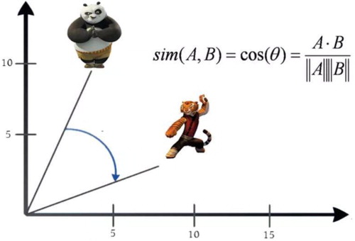
• In the last section, the conclusion of the manuscript is discussed. The graphical representation of the similarity measures are discussed in the form of Figure 1.

Figure 1. Geometrical representation of the cosine similarity measures.

The remainder of this manuscript is divided many section. In Section 1, we discussed the history of the article in detailed. In Section 2, some basic definitions and notion related to this article are studied. Section 3, the authors introduced the concept of SMs for PHFSs based on cosine and cotangent functions. Section 4 is based on the application of the proposed work and their results and discussed. Section is based on comparative study, we have some advantages of the new work defined so far in Section 3. Finally, the article ends with some future directions.

2. Preliminaries

In the following, we introduced some basic definitions and notion related to IFSs, PFSs, HFSs, PHFSs. Further, we studied some SMs of IFSs and PFSs with based on cosine and cotangent functions. In our study by $X$ we mean the universal set and $\alpha ,\eta and\text{β}$ denote the degrees of membership, indeterminacy and non-membership on a scale of 0 to 1. Moreover, the notation ‘$\vee$’ is denote the maximum operation and the set of all PHFNs on $X$ denoted by PHFS$\left(X\right)$.

Definition 1:

[2] An IFS $A$ on $X$ is of the form $A=\left\{〈x,{\alpha }_A\left(x\right),{\text{β}}_A\left(x\right)〉|x\in X\right\}$, where ${\alpha }_A:X\to \left[0,1\right]$ and ${\text{β}}_A:X\to \left[0,1\right]$ such that $0\le {\alpha }_A\left(x\right)+{\text{β}}_A\left(x\right)\le 1$. Further ${\delta }_A\left(x\right)=1-\left({\alpha }_A\left(x\right)+{\text{β}}_A\left(x\right)\right)$ is called the degree of hesitancy of $x\in X$ in the set $A$. For convenience, the intuitionistic fuzzy number (IFN) is denoted by $\left(\alpha ,\text{β},\delta \right)$.

In real life, there is some problem which could not be symbolised in IFS theory. For example, in the situation of voting system, human opinions including more answers of such types: yes, no, abstain, refusal. Therefore, Cuong [11] enclosed these gaps by adding the neutral function in IFS theory, Cuong [1] presented the core idea of the PFS model, and the PFS notion is the extension of IFS model. In PFS theory, he basically added the neutral term along with the positive membership degree and negative membership degree of the IFS theory. The only constraint is that in PFS theory, the sum of the positive membership, neutral and negative membership degrees of the function is equal to or less than 1.

Definition 2

: [11] A PFS $A$ on $X$ is of the form $A=\left\{〈x,{\alpha }_A\left(x\right),{\eta }_A\left(x\right),{\text{β}}_A\left(x\right)〉|x\in X\right\}$, where ${\alpha }_A:X\to \left[0,1\right]$, ${\eta }_A:X\to \left[0,1\right]$ and ${\text{β}}_A:X\to \left[0,1\right]$ such that $0\le {\alpha }_A\left(x\right)+{\eta }_A\left(x\right)+{\text{β}}_A\left(x\right)\le 1$. Further ${\delta }_A\left(x\right)=1-\left({\alpha }_A\left(x\right)+{\eta }_A\left(x\right)+{\text{β}}_A\left(x\right)\right)$ is called the degree of hesitancy of $x\in X$ in the set $A$. For convenience, the picture fuzzy number (PFN) is denoted by$\left(\alpha ,\eta ,\text{β},\delta \right)$.

The theory of FS have received extensive attention form scholars and numerous researchers have utilised in the environment of different fields [1,2]. But, there was some complications, when a decision maker provides the information’s in the form of subset of unit interval, then the theory of FS cannot able to cope with it. For coping with such types of issues, the theory of hesitant fuzzy sets was presented by Torra [16] which is discussed below.

Definition 3:

[16] A HFS $A$ on $X$ is of the form $A=\left\{〈x,{\mathcal{H}}_A\left(x\right)〉|x\in X\right\}$, where ${\mathcal{H}}_A:X\to \left[0,1\right]$ denote the set of finite values of $x\in X$ in the set $A$. For convenience, the hesitant fuzzy number (HFN) is denoted by $\left(\mathcal{H}\right)$.

The theories of FS, IFS, PFS and HFS have received extensive attention form scholars and numerous researchers have utilised in the environment of different fields [1–2]. But, there was some complications, when a decision maker provides the information’s for the grade of truth, the grade of abstinence, and the grade of falsity in the form of subset of unit interval, then the theory of exiting theories are cannot able to cope with it. For coping with such types of issues the theory of PHFSs was presented by Ahmad et al. [44] which is discussed below.

Definition 4:

[44] A PHFS $A$ on $X$ is of the form $A=\left\{〈x,{\alpha }_A\left(x\right),{\eta }_A\left(x\right),{\text{β}}_A\left(x\right)〉|x\in X\right\}$, where ${\alpha }_A:X\to \left[0,1\right]$, ${\eta }_A:X\to \left[0,1\right]$ and ${\text{β}}_A:X\to \left[0,1\right]$ such that $0\le \text{Sup}\left({\alpha }_A\left(x\right)\right)+\text{Sup}\left({\eta }_A\left(x\right)\right)+\text{Sup}\left({\text{β}}_A\left(x\right)\right)\le 1.$ Further, ${\delta }_A\left(x\right)=1-\left(\text{Sup}\right({\alpha }_A\left(x\right))+\text{Sup}({\eta }_A\left(x\right))+\text{Sup}({\text{β}}_A\left(x\right)\left)\right)$ is called the degree of hesitancy of $x\in X$in the set $A$. For convenience, the picture hesitant fuzzy number (PHFN) is denoted by $\left(\alpha ,\eta ,\text{β},\delta \right)$.

Definition 5:

[34] For two IFNs $A=\left({\alpha }_A,{\text{β}}_A\right)$ and $B=\left({\alpha }_B,{\text{β}}_B\right)$ on $X$, a cosine SM is defined as: (1) $\text{IF}{\text{C}}^1\left(A,B\right)=\frac{1}{m}\sum _{i=1}^m\frac{{\alpha }_A\left(x_i\right){\alpha }_B\left(x_i\right)+{\text{β}}_A\left(x_i\right){\text{β}}_B\left(x_i\right)}{\sqrt{{\alpha }_A^2\left(x_i\right)+{\text{β}}_A^2\left(x_i\right)}\sqrt{{\alpha }_B^2\left(x_i\right)+{\text{β}}_B^2\left(x_i\right)}}$(1)

Definition 6:

[34] For two IFNs $A=\left({\alpha }_A,{\text{β}}_A\right)$ and $B=\left({\alpha }_B,{\text{β}}_B\right)$ on $X$ based on the cosine function, then SMs are defined as: (2) $\text{IFC}{\text{S}}^1\left(A,B\right)=\frac{1}{m}\sum _{i=1}^m\text{cos}\left[\frac{\pi }{2}\left(|{\alpha }_A\left(x_i\right)-{\alpha }_B\left(x_i\right)|\vee |{\text{β}}_A\left(x_i\right)-{\text{β}}_B\left(x_i\right)|\right)\right]$(2) (3) $\text{IFC}{\text{S}}^2\left(A,B\right)=\frac{1}{m}\sum _{i=1}^m\text{cos}\left[\frac{\pi }{4}\left(|{\alpha }_A\left(x_i\right)-{\alpha }_B\left(x_i\right)|+|{\text{β}}_A\left(x_i\right)-{\text{β}}_B\left(x_i\right)|\right)\right]$(3)

Definition 7:

[34] For two IFNs $A=\left({\alpha }_A,{\text{β}}_A\right)$ and $B=\left({\alpha }_B,{\text{β}}_B\right)$ on $X$ based on the cotangent function, then SM is defined as: (4) $\text{IFC}{\text{T}}^1\left(A,B\right)=\frac{1}{m}\sum _{i=1}^m\text{cot}\left[\frac{\pi }{4}+\frac{\pi }{4}\left(|{\alpha }_A\left(x_i\right)-{\alpha }_B\left(x_i\right)|\vee |{\text{β}}_A\left(x_i\right)-{\text{β}}_B\left(x_i\right)|\right)\right]$(4)

Definition 8:

[36] For two PFNs $A=\left({\alpha }_A,{\eta }_A,{\text{β}}_A\right)$ and $B=\left({\alpha }_B,{\eta }_B,{\text{β}}_B\right)$ on $X$, a cosine SM is defined as: (5) $\text{PF}{\text{C}}^1\left(A,B\right)=\frac{1}{m}\sum _{i=1}^m\frac{{\alpha }_A\left(x_i\right){\alpha }_B\left(x_i\right)+{\eta }_A\left(x_i\right){\eta }_B\left(x_i\right)+{\text{β}}_A\left(x_i\right){\text{β}}_B\left(x_i\right)}{\sqrt{{\alpha }_A^2\left(x_i\right)+{\eta }_A^2\left(x_i\right)+{\text{β}}_A^2\left(x_i\right)}\sqrt{{\alpha }_B^2\left(x_i\right)+{\eta }_B^2\left(x_i\right)+{\text{β}}_B^2\left(x_i\right)}}$(5)

Definition 9:

[36] For two PFNs $A=\left({\alpha }_A,{\eta }_A,{\text{β}}_A\right)$ and $B=\left({\alpha }_B,{\eta }_B,{\text{β}}_B\right)$ on $X$ based on the cosine function, then SMs are defined as: (6) $\text{PFC}{\text{S}}^1\left(A,B\right)=\frac{1}{m}\sum _{i=1}^m\text{cos}\left[\frac{\pi }{2}\left(|{\alpha }_A\left(x_i\right)-{\alpha }_B\left(x_i\right)|\vee |{\eta }_A\left(x_i\right)-{\eta }_B\left(x_i\right)|\vee |{\text{β}}_A\left(x_i\right)-{\text{β}}_B\left(x_i\right)|\right)\right]$(6) (7) $\text{PFC}{\text{S}}^2\left(A,B\right)=\frac{1}{m}\sum _{i=1}^m\text{cos}\left[\frac{\pi }{4}\left(|{\alpha }_A\left(x_i\right)-{\alpha }_B\left(x_i\right)|+|{\eta }_A\left(x_i\right)-{\eta }_B\left(x_i\right)|+|{\text{β}}_A\left(x_i\right)-{\text{β}}_B\left(x_i\right)|\right)\right]$(7)

Definition 10:

[36] For two PFNs $A=\left({\alpha }_A,{\eta }_A,{\text{β}}_A\right)$ and $B=\left({\alpha }_B,{\eta }_B,{\text{β}}_B\right)$ on $X$ based on the cotangent function, then SM is defined as: (8) $\text{PFC}{\text{T}}^1\left(A,B\right)=\frac{1}{m}\sum _{i=1}^m\text{cot}\left[\frac{\pi }{4}+\frac{\pi }{4}\left(|{\alpha }_A\left(x_i\right)-{\alpha }_B\left(x_i\right)|\vee |{\eta }_A\left(x_i\right)-{\eta }_B\left(x_i\right)|\vee |{\text{β}}_A\left(x_i\right)-{\text{β}}_B\left(x_i\right)|\right)\right]$(8)

Definition 11:

[38] For a HFS on the universal set $X$. $S\left(\mathcal{H}\left(x\right)\right)=\frac{1}{l\mathcal{H}\left(x\right)}\sum _{\gamma \in \mathcal{H}\left(x\right)}\gamma$ is called the score function of $\mathcal{H}\left(x\right)$, where $\gamma$ denotes the element in $\mathcal{H}\left(x\right)$ and $l\mathcal{H}\left(x\right)$ denote the number of element in $\mathcal{H}\left(x\right)$.

Now we define the inclusion of two PHFSs.

Definition 12:

[27] Let $A$ and $B$ be the PHFSs. Then $A\subseteq B$iff

• $S\left({\alpha }_A\left(x\right)\right)\le S\left({\alpha }_B\left(x\right)\right)\Rightarrow {\alpha }_A\left(x\right)\le {\alpha }_B\left(x\right)$

• $S\left({\eta }_A\left(x\right)\right)\le S\left({\eta }_B\left(x\right)\right)\Rightarrow {\eta }_A\left(x\right)\le {\eta }_B\left(x\right)$

• $S\left({\text{β}}_A\left(x\right)\right)\ge S\left({\text{β}}_B\left(x\right)\right)\Rightarrow {\text{β}}_A\left(x\right)\ge {\text{β}}_B\left(x\right)$

3. SMs Based on Cosine and Cotangent Functions for PHFSs

The aim of this section is to develop some SMs for PHFSs including cosine SM for PHFSs, cosine SMs of PHFSs based on cosine and cotangent functions. The new approaches of SMs developed from here are more general and reliable with the existing SMs defined in Equations (1)–(8). Further, with the help of some remarks we introduced the idea of SMs for IHFSs. In our study $l{\alpha }_A$ mean the length of ${\alpha }_A$ and similar. Moreover, ${\alpha }^{\ast }$, ${\eta }^{\ast }$, ${\text{β}}^{\ast }$ and ${\delta }^{\ast }$ denote the length and defined as: ${\alpha }^{\ast }=\text{max}\left(l{\alpha }_A,l{\alpha }_B\right)$, ${\eta }^{\ast }=\text{max}\left(l{\eta }_A,l{\eta }_B\right)$, ${\text{β}}^{\ast }=\text{max}\left(l{\text{β}}_A,l{\text{β}}_B\right)$ and ${\delta }^{\ast }=\text{max}\left(l{\delta }_A,l{\delta }_B\right)$, respectively.

3.1. Cosine SMs for PHFSs.

In this study, we claim that the works proposed in this section are general and reliable of the existing SMs discussed in References [34,36].

Definition 13:

For two PHFNs $A=\left({\alpha }_A,{\eta }_A,{\text{β}}_A\right)$ and $B=\left({\alpha }_B,{\eta }_B,{\text{β}}_B\right)$ on $X$, a cosine SM is defined as: (9) $\text{PHF}{\text{C}}^1\left(A,B\right)=\frac{1}{n}\sum _{i=1}^n\frac{\frac{1}{{\alpha }^{\ast }}\sum _{j=1}^{{\alpha }^{\ast }}{{\alpha }^j}_A\left(x_i\right){\alpha }_B^j\left(x_i\right)+\frac{1}{{\eta }^{\ast }}\sum _{k=1}^{{\eta }^{\ast }}{\eta }_A^k\left(x_i\right){\eta }_B^k\left(x_i\right)+\frac{1}{{\text{β}}^{\ast }}\sum _{m=1}^{{\text{β}}^{\ast }}{\text{β}}_A^m\left(x_i\right){\text{β}}_B^m\left(x_i\right)}{\sqrt{\begin{array}{c}\frac{1}{{\alpha }^{\ast }}\sum _{j=1}^{{\alpha }^{\ast }}{\left({{\alpha }^j}_A\left(x_i\right)\right)}^2\\ +\frac{1}{{\eta }^{\ast }}\sum _{k=1}^{{\eta }^{\ast }}{\left({\eta }_A^k\left(x_i\right)\right)}^2\\ +\frac{1}{{\text{β}}^{\ast }}\sum _{m=1}^{{\text{β}}^{\ast }}{\left({\text{β}}_A^m\left(x_i\right)\right)}^2\end{array}}\cdot \sqrt{\begin{array}{c}\frac{1}{{\alpha }^{\ast }}\sum _{j=1}^{{\alpha }^{\ast }}{\left({\alpha }_B^j\left(x_i\right)\right)}^2\\ +\frac{1}{{\eta }^{\ast }}\sum _{k=1}^{{\eta }^{\ast }}{\left({\eta }_B^k\left(x_i\right)\right)}^2\\ +\frac{1}{{\text{β}}^{\ast }}\sum _{m=1}^{{\text{β}}^{\ast }}{\left({\text{β}}_B^m\left(x_i\right)\right)}^2\end{array}}}$(9) The cosine SM for PHFSs $A,B$ and $C$ satisfy following conditions of SMs:

1. $0\le \text{PHF}{\text{C}}^1\left(A,B\right)\le 1$

2. $\text{PHF}{\text{C}}^1\left(A,B\right)=\text{PHF}{\text{C}}^1\left(B,A\right)$

3. $\text{PHF}{\text{C}}^1\left(A,B\right)=1\text{iff}A=B$

4. If $A\subseteq B\subseteq C$, then $\text{PHF}{\text{C}}^1\left(A,C\right)\le \text{PHF}{\text{C}}^1\left(A,B\right)$ and $\text{PHF}{\text{C}}^1\left(A,C\right)\le \text{PHF}{\text{C}}^1\left(B,C\right)$.

Proof:

First and second conditions proof are obvious.

Now, we are going to prove the third condition, if we take $A=B$ that is ${\alpha }_A^j\left(x_i\right)={\alpha }_B^j\left(x_i\right)$, ${\eta }_A^k\left(x_i\right)={\eta }_B^k\left(x_i\right)$ and ${\text{β}}_A^m\left(x_i\right)={\text{β}}_B^m\left(x_i\right)$ for $i=1,2,\dots ,n$. Therefore Equation (9) implies $\begin{array}{rl}\text{PHF}{\text{C}}^1\left(A,B\right)& =\frac{1}{n}\sum _{i=1}^n\left(\frac{\frac{1}{{\alpha }^{\ast }}\sum _{j=1}^{{\alpha }^{\ast }}{{\alpha }^j}_A\left(x_i\right){\alpha }_A^j\left(x_i\right)+\frac{1}{{\eta }^{\ast }}\sum _{k=1}^{{\eta }^{\ast }}{\eta }_A^k\left(x_i\right){\eta }_A^k\left(x_i\right)+\frac{1}{{\text{β}}^{\ast }}\sum _{m=1}^{{\text{β}}^{\ast }}{\text{β}}_A^m\left(x_i\right){\text{β}}_A^m\left(x_i\right)}{\sqrt{\begin{array}{c}\frac{1}{{\alpha }^{\ast }}\sum _{j=1}^{{\alpha }^{\ast }}{\left({{\alpha }^j}_A\left(x_i\right)\right)}^2\\ +\frac{1}{{\eta }^{\ast }}\sum _{k=1}^{{\eta }^{\ast }}{\left({\eta }_A^k\left(x_i\right)\right)}^2\\ +\frac{1}{{\text{β}}^{\ast }}\sum _{m=1}^{{\text{β}}^{\ast }}{\left({\text{β}}_A^m\left(x_i\right)\right)}^2\end{array}}.\sqrt{\begin{array}{c}\frac{1}{{\alpha }^{\ast }}\sum _{j=1}^{{\alpha }^{\ast }}{\left({\alpha }_A^j\left(x_i\right)\right)}^2\\ +\frac{1}{{\eta }^{\ast }}\sum _{k=1}^{{\eta }^{\ast }}{\left({\eta }_A^k\left(x_i\right)\right)}^2\\ +\frac{1}{{\text{β}}^{\ast }}\sum _{m=1}^{{\text{β}}^{\ast }}{\left({\text{β}}_A^m\left(x_i\right)\right)}^2\end{array}}}\right)\\ & =\frac{1}{n}\sum _{i=1}^n\left(\frac{\frac{1}{{\alpha }^{\ast }}{\sum }_{j=1}^{{\alpha }^{\ast }}{\left({{\alpha }^j}_A\left(x_i\right)\right)}^2+\frac{1}{{\eta }^{\ast }}{\sum }_{k=1}^{{\eta }^{\ast }}{\left({\eta }_A^k\left(x_i\right)\right)}^2+\frac{1}{{\text{β}}^{\ast }}{\sum }_{m=1}^{{\text{β}}^{\ast }}{\left({\text{β}}_A^m\left(x_i\right)\right)}^2}{\frac{1}{{\alpha }^{\ast }}{\sum }_{j=1}^{{\alpha }^{\ast }}{\left({{\alpha }^j}_A\left(x_i\right)\right)}^2+\frac{1}{{\eta }^{\ast }}{\sum }_{k=1}^{{\eta }^{\ast }}{\left({\eta }_A^k\left(x_i\right)\right)}^2+\frac{1}{{\text{β}}^{\ast }}{\sum }_{m=1}^{{\text{β}}^{\ast }}{\left({\text{β}}_A^m\left(x_i\right)\right)}^2}\right)=1\end{array}$ For condition no. $\left(4\right)$, let $A,BandC\in \text{PHFS}\left(X\right)$. We know that, if

• $S\left({\alpha }_A\left(x\right)\right)\le S\left({\alpha }_B\left(x\right)\right)\le S\left({\alpha }_C\left(x\right)\right)\Rightarrow {\alpha }_A\left(x\right)\le {\alpha }_B\left(x\right)\le {\alpha }_C\left(x\right)$

• $S\left({\eta }_A\left(x\right)\right)\le S\left({\eta }_B\left(x\right)\right)\le S\left({\eta }_C\left(x\right)\right)\Rightarrow {\eta }_A\left(x\right)\le {\eta }_B\left(x\right)\le {\alpha }_C\left(x\right)$

• $S\left({\text{β}}_A\left(x\right)\right)\ge S\left({\text{β}}_B\left(x\right)\right)\ge S\left({\text{β}}_B\left(x\right)\right)\Rightarrow {\text{β}}_A\left(x\right)\ge {\text{β}}_B\left(x\right)\ge {\alpha }_C\left(x\right)$ for each $x\in X$.

$\Rightarrow A\subseteq B\subseteq C$. Hence $\text{PHF}{\text{C}}^1\left(A,C\right)\le \text{PHF}{\text{C}}^1\left(A,B\right)$ and $\text{PHF}{\text{C}}^1\left(A,C\right)\le \text{PHF}{\text{C}}^1\left(B,C\right)$

Definition 14:

For two PHFNs $A=\left({\alpha }_A,{\eta }_A,{\text{β}}_A\right)$ and $B=\left({\alpha }_B,{\eta }_B,{\text{β}}_B\right)$ on $X$, a weighted cosine SM is defined as: (10) $\text{WPHF}{\text{C}}^1\left(A,B\right)=\sum _{i=1}^{\pi }{\omega }_i\left(\frac{\frac{1}{{\alpha }^{\ast }}\sum _{j=1}^{{\alpha }^{\ast }}{{\alpha }^j}_A\left(x_i\right){\alpha }_B^j\left(x_i\right)+\frac{1}{{\eta }^{\ast }}\sum _{k=1}^{{\eta }^{\ast }}{\eta }_A^k\left(x_i\right){\eta }_B^k\left(x_i\right)+\frac{1}{{\text{β}}^{\ast }}\sum _{m=1}^{{\text{β}}^{\ast }}{\text{β}}_A^m\left(x_i\right){\text{β}}_B^m\left(x_i\right)}{\sqrt{\begin{array}{c}\frac{1}{{\alpha }^{\ast }}\sum _{j=1}^{{\alpha }^{\ast }}{\left({{\alpha }^j}_A\left(x_i\right)\right)}^2\\ +\frac{1}{{\eta }^{\ast }}\sum _{k=1}^{{\eta }^{\ast }}{\left({\eta }_A^k\left(x_i\right)\right)}^2\\ +\frac{1}{{\text{β}}^{\ast }}\sum _{m=1}^{{\text{β}}^{\ast }}{\left({\text{β}}_A^m\left(x_i\right)\right)}^2\end{array}}.\sqrt{\begin{array}{c}\frac{1}{{\alpha }^{\ast }}\sum _{j=1}^{{\alpha }^{\ast }}{\left({\alpha }_B^j\left(x_i\right)\right)}^2\\ +\frac{1}{{\eta }^{\ast }}\sum _{k=1}^{{\eta }^{\ast }}{\left({\eta }_B^k\left(x_i\right)\right)}^2\\ +\frac{1}{{\text{β}}^{\ast }}\sum _{m=1}^{{\text{β}}^{\ast }}{\left({\text{β}}_B^m\left(x_i\right)\right)}^2\end{array}}}\right)$(10) In the following, $\omega =({\omega }_1,{\omega }_2,\dots ,{\omega }_m{)}^{\text{T}}$ denotes a weighted vector were ${\omega }_i$ must belong on a scale of 0 to 1 and the sum of ${\omega }_i$ is equal to 1. By taking ${\omega }_i=\frac{1}{m}$ then Equation (10) reduced to Equation (9). The weighted cosine SM for PHFNs $A$ and $B$ satisfy following results:

1. $0\le \text{WPHF}{\text{C}}^1\left(A,B\right)\le 1$

2. $\text{WPHF}{\text{C}}^1\left(A,B\right)=\text{WPHF}{\text{C}}^1\left(B,A\right)$

3. $\text{WPHF}{\text{C}}^1\left(A,B\right)=1\text{iff }A=B$

Proof:

Proof is straight forward.

Definition 15:

For two PHFNs $A=\left({\mu }_A,{\eta }_A,{\upsilon }_A,{\delta }_A\right)$ and $B=\left({\mu }_B,{\eta }_B,{\upsilon }_B,{\delta }_B\right)$ on $X$, then a cosine SM and a weighted cosine SM are defined as: (11) $\begin{array}{rl}& \text{PHF}{\text{C}}^2\left(A,B\right)\\ & =\frac{1}{n}\sum _{t=1}^n\left(\frac{\begin{array}{c}\frac{1}{{\alpha }^{\ast }}\sum _{j=1}^{{\alpha }^{\ast }}{{\alpha }^j}_A\left(x_i\right){\alpha }_B^j\left(x_i\right)+\frac{1}{{\eta }^{\ast }}\sum _{k=1}^{{\eta }^{\ast }}{\eta }_A^k\left(x_i\right){\eta }_B^k\left(x_i\right)+\frac{1}{{\text{β}}^{\ast }}\sum _{m=1}^{{\text{β}}^{\ast }}{\text{β}}_A^m\left(x_i\right){\text{β}}_B^m\left(x_i\right)\\ +\frac{1}{{\delta }^{\ast }}\sum _{o=1}^{{\delta }^{\ast }}{\delta }_A^o\left(x_i\right){\delta }_B^o\left(x_i\right)\end{array}}{\sqrt{\begin{array}{c}\frac{1}{{\alpha }^{\ast }}\sum _{j=1}^{{\alpha }^{\ast }}{\left({{\alpha }^j}_A\left(x_i\right)\right)}^2+\frac{1}{{\eta }^{\ast }}\sum _{k=1}^{{\eta }^{\ast }}{\left({\eta }_A^k\left(x_i\right)\right)}^2\\ +\frac{1}{{\text{β}}^{\ast }}\sum _{m=1}^{{\text{β}}^{\ast }}{\left({\text{β}}_A^m\left(x_i\right)\right)}^2+\frac{1}{{\delta }^{\ast }}\sum _{o=1}^{{\delta }^{\ast }}{\left({\delta }_A^o\left(x_i\right)\right)}^2\end{array}}.\sqrt{\begin{array}{c}\frac{1}{{\alpha }^{\ast }}\sum _{j=1}^{{\alpha }^{\ast }}{\left({{\alpha }^j}_B\left(x_i\right)\right)}^2+\frac{1}{{\eta }^{\ast }}\sum _{k=1}^{{\eta }^{\ast }}{\left({\eta }_B^k\left(x_i\right)\right)}^2\\ +\frac{1}{{\text{β}}^{\ast }}\sum _{m=1}^{{\text{β}}^{\ast }}{\left({\text{β}}_B^m\left(x_i\right)\right)}^2+\frac{1}{{\delta }^{\ast }}\sum _{o=1}^{{\delta }^{\ast }}{\left({\delta }_B^o\left(x_i\right)\right)}^2\end{array}}}\right)\end{array}$(11) (12) $\begin{array}{l}\text{WPHF}{\text{C}}^2\left(A,B\right)\\ =\sum _{i=1}^n{\omega }_i\left(\frac{\begin{array}{c}\frac{1}{{\alpha }^{\ast }}\sum _{j=1}^{{\alpha }^{\ast }}{{\alpha }^j}_A\left(x_i\right){\alpha }_B^j\left(x_i\right)+\frac{1}{{\eta }^{\ast }}\sum _{k=1}^{{\eta }^{\ast }}{\eta }_A^k\left(x_i\right){\eta }_B^k\left(x_i\right)+\frac{1}{{\text{β}}^{\ast }}\sum _{m=1}^{{\text{β}}^{\ast }}{\text{β}}_A^m\left(x_i\right){\text{β}}_B^m\left(x_i\right)\\ +\frac{1}{{\delta }^{\ast }}\sum _{o=1}^{{\delta }^{\ast }}{\delta }_A^o\left(x_i\right){\delta }_B^o\left(x_i\right)\end{array}}{\sqrt{\begin{array}{c}\frac{1}{{\alpha }^{\ast }}\sum _{j=1}^{{\alpha }^{\ast }}{\left({{\alpha }^j}_A\left(x_i\right)\right)}^2+\frac{1}{{\eta }^{\ast }}\sum _{k=1}^{{\eta }^{\ast }}{\left({\eta }_A^k\left(x_i\right)\right)}^2\\ +\frac{1}{{\text{β}}^{\ast }}\sum _{m=1}^{{\text{β}}^{\ast }}{\left({\text{β}}_A^m\left(x_i\right)\right)}^2+\frac{1}{{\delta }^{\ast }}\sum _{o=1}^{{\delta }^{\ast }}{\left({\delta }_A^o\left(x_i\right)\right)}^2\end{array}}.\sqrt{\begin{array}{c}\frac{1}{{\alpha }^{\ast }}\sum _{j=1}^{{\alpha }^{\ast }}{\left({{\alpha }^j}_B\left(x_i\right)\right)}^2+\frac{1}{{\eta }^{\ast }}\sum _{k=1}^{{\eta }^{\ast }}{\left({\eta }_B^k\left(x_i\right)\right)}^2\\ +\frac{1}{{\text{β}}^{\ast }}\sum _{m=1}^{{\text{β}}^{\ast }}{\left({\text{β}}_B^m\left(x_i\right)\right)}^2+\frac{1}{{\delta }^{\ast }}\sum _{o=1}^{{\delta }^{\ast }}{\left({\delta }_B^o\left(x_i\right)\right)}^2\end{array}}}\right)\end{array}$(12)

Proof:

Similar

Remark 1:

If

• We assume that ${\eta }_A={\eta }_B=\left\{0\right\}$, then $\text{PHF}{\text{C}}^{\text{1}}$ will become to $\text{IHF}{\text{C}}^{\text{1}}$and write as: $\text{IHF}{\text{C}}^1\left(A,B\right)=\frac{1}{n}\sum _{i=1}^n\left(\frac{\frac{1}{{\alpha }^{\ast }}\sum _{j=1}^{{\alpha }^{\ast }}{{\alpha }^j}_A\left(x_i\right){\alpha }_B^j\left(x_i\right)+\frac{1}{{\text{β}}^{\ast }}\sum _{m=1}^{{\text{β}}^{\ast }}{\text{β}}_A^m\left(x_i\right){\text{β}}_B^m\left(x_i\right)}{\sqrt{\begin{array}{c}\frac{1}{{\alpha }^{\ast }}\sum _{j=1}^{{\alpha }^{\ast }}{\left({\alpha }_A^j\left(x_i\right)\right)}^2\\ +\frac{1}{{\text{β}}^{\ast }}\sum _{m=1}^{{\text{β}}^{\ast }}{\left({\text{β}}_A^m\left(x_i\right)\right)}^2\end{array}}\cdot \sqrt{\begin{array}{c}\frac{1}{{\alpha }^{\ast }}\sum _{j=1}^{{\alpha }^{\ast }}{\left({\alpha }_B^j\left(x_i\right)\right)}^2\\ +\frac{1}{{\text{β}}^{\ast }}\sum _{m=1}^{{\text{β}}^{\ast }}{\left({\text{β}}_B^m\left(x_i\right)\right)}^2\end{array}}}\right)$

• We assume that ${\eta }_A={\eta }_B=\left\{0\right\}$, then $\text{PHF}{\text{C}}^{\text{2}}$ will become to $\text{IHF}{\text{C}}^2$ and write as: $\text{IHF}{\text{C}}^2\left(A,B\right)=\frac{1}{n}\sum _{i=1}^{\pi }\left(\frac{\frac{1}{{\alpha }^{\ast }}\sum _{j=1}^{{\alpha }^{\ast }}{{\alpha }^j}_A\left(x_i\right){\alpha }_B^j\left(x_i\right)+\frac{1}{{\text{β}}^{\ast }}\sum _{m=1}^{{\text{β}}^{\ast }}{\text{β}}_A^m\left(x_i\right){\text{β}}_B^m\left(x_i\right)+\frac{1}{{\delta }^{\ast }}\sum _{o=1}^{{\delta }^{\ast }}{\delta }_A^o\left(x_i\right){\delta }_B^o\left(x_i\right)}{\sqrt{\begin{array}{c}\frac{1}{{\alpha }^{\ast }}\sum _{j=1}^{{\alpha }^{\ast }}{\left({\alpha }_A^j\left(x_i\right)\right)}^2\\ +\frac{1}{{\text{β}}^{\ast }}\sum _{m=1}^{{\text{β}}^{\ast }}{\left({\text{β}}_A^m\left(x_i\right)\right)}^2\\ +\frac{1}{{\delta }^{\ast }}\sum _{o=1}^{{\delta }^{\ast }}{\left({\delta }_A^o\left(x_i\right)\right)}^2\end{array}}.\sqrt{\begin{array}{c}\frac{1}{{\alpha }^{\ast }}\sum _{j=1}^{{\alpha }^{\ast }}{\left({\alpha }_B^j\left(x_i\right)\right)}^2\\ +\frac{1}{{\text{β}}^{\ast }}\sum _{m=1}^{{\text{β}}^{\ast }}{\left({\text{β}}_B^m\left(x_i\right)\right)}^2\\ +\frac{1}{{\delta }^{\ast }}\sum _{o=1}^{{\delta }^{\ast }}{\left({\delta }_B^o\left(x_i\right)\right)}^2\end{array}}}\right)$

3.2. SMs for PHFSs Based on Cosine Function

In this portion, we shall propose SMs for PHFSs based on cosine function which are the generalisation of the existing SMs defined in Equations (2) and (3) and Equations (6) and (7).

Definition 16:

For two PHFNs $A=\left({\alpha }_A,{\eta }_A,{\text{β}}_A\right)$ and $B=\left({\alpha }_B,{\eta }_B,{\text{β}}_B\right)$ on $X$ based on the cosine function, then SMs are defined as: (13) $\text{PHFC}{\text{S}}^1\left(A,B\right)=\frac{1}{n}\sum _{i=1}^n\text{cos}\left[\frac{\pi }{2}\left(\begin{array}{c}\frac{1}{{\alpha }^{\ast }}\sum _{j=1}^{{\alpha }^{\ast }}|{{\alpha }^j}_A\left(x_i\right)-{\alpha }_B^j\left(x_i\right)|\vee \frac{1}{{\eta }^{\ast }}\sum _{k=1}^{{\eta }^{\ast }}|{\eta }_A^k\left(x_i\right)-{\eta }_B^k\left(x_i\right)|\\ \vee \frac{1}{{\text{β}}^{\ast }}\sum _{m=1}^{{\text{β}}^{\ast }}|{\text{β}}_A^m\left(x_i\right)-{\text{β}}_B^m\left(x_i\right)|\end{array}\right)\right]$(13) (14) $\text{PHFC}{\text{S}}^2\left(A,B\right)=\frac{1}{n}\sum _{i=1}^{\pi }\cos \left[\frac{\pi }{4}\left(\begin{array}{l}\frac{1}{{\alpha }^{\ast }}\sum _{j=1}^{{\alpha }^{\ast }}|{{\alpha }^j}_A\left(x_i\right)-{\alpha }_B^j\left(x_i\right)|+\frac{1}{{\eta }^{\ast }}\sum _{k=1}^{{\eta }^{\ast }}|{\eta }_A^k\left(x_i\right)-{\eta }_B^k\left(x_i\right)|\\ +\frac{1}{{\text{β}}^{\ast }}\sum _{m=1}^{{\text{β}}^{\ast }}|{\text{β}}_A^m\left(x_i\right)-{\text{β}}_B^m\left(x_i\right)|\end{array}\right)\right]$(14) The SMs for PHFNs $A,B$ and $C$ based on cosine function satisfy the following results of SMs:

1. $0\le \text{PHFC}{\text{S}}^{1,2}\left(A,B\right)\le 1$

2. $\text{PHFC}{\text{S}}^{1,2}\left(A,B\right)=\text{PHFC}{\text{S}}^{1,2}\left(B,A\right)$

3. $\text{PHFC}{\text{S}}^{1,2}\left(A,B\right)=1\text{ iff}A=B$

4. If $A\subseteq B\subseteq C$, then $\text{PHFC}{\text{S}}^{1,2}\left(A,C\right)\le \text{PHFC}{\text{S}}^{1,2}\left(A,B\right)$ and $\text{PHFC}{\text{S}}^{1,2}\left(A,C\right)\le \text{PHFC}{\text{S}}^{1,2}\left(B,C\right)$.

Proof:

The first and second conditions proof are obvious.

Now, we are going to prove the third condition, if we take $A=B$ that is ${\alpha }_A^j\left(x_i\right)={\alpha }_B^j\left(x_i\right)$, ${\eta }_A^k\left(x_i\right)={\eta }_B^k\left(x_i\right)$ and ${\text{β}}_A^m\left(x_i\right)={\text{β}}_B^m\left(x_i\right)$ for $i=1,2,\dots ,n$. Therefore, Equations (13) and (14) imply that $\frac{1}{{\alpha }^{\ast }}\sum _{j=1}^{{\alpha }^{\ast }}|{{\alpha }^j}_A\left(x_i\right)-{\alpha }_A^j\left(x_i\right)|=0$, $\frac{1}{{\eta }^{\ast }}\sum _{k=1}^{{\eta }^{\ast }}|{\eta }_A^k\left(x_i\right)-{\eta }_A^k\left(x_i\right)|=0$ and $\frac{1}{{\text{β}}^{\ast }}\sum _{m=1}^{{\text{β}}^{\ast }}|{\text{β}}_A^m\left(x_i\right)-{\text{β}}_A^m\left(x_i\right)|=0$. So, $\text{PHFC}{\text{S}}^{1,2}\left(A,B\right)=1$. But on the other hand, if we take $\text{PHFC}{\text{S}}^{1,2}\left(A,B\right)=1$, then this implies that $\frac{1}{{\alpha }^{\ast }}\sum _{j=1}^{{\alpha }^{\ast }}|{{\alpha }^j}_A\left(x_i\right)-{\alpha }_B^j\left(x_i\right)|=0$, $\frac{1}{{\eta }^{\ast }}\sum _{k=1}^{{\eta }^{\ast }}|{\eta }_A^k\left(x_i\right)-{\eta }_B^k\left(x_i\right)|=0$ and $\frac{1}{{\text{β}}^{\ast }}\sum _{m=1}^{{\text{β}}^{\ast }}|{\text{β}}_A^m\left(x_i\right)-{\text{β}}_B^m\left(x_i\right)|=0$. Since we know that $\cos \left(0\right)=1$. Then, there are ${\alpha }_A^j\left(x_i\right)={\alpha }_B^j\left(x_i\right)$, ${\eta }_A^k\left(x_i\right)={\eta }_B^k\left(x_i\right)$ and ${\text{β}}_A^m\left(x_i\right)={\text{β}}_B^m\left(x_i\right)$ for $i=1,2,\dots ,n$. Hence $A=B$.

For condition no. 4, if $A\subseteq B\subseteq C$, then there are ${\alpha }_A^j\left(x_i\right)\le {\alpha }_B^j\left(x_i\right)\le {\alpha }_C^j\left(x_i\right)$, ${\eta }_A^k\left(x_i\right)\le {\eta }_B^k\left(x_i\right)\le {\eta }_C^k\left(x_i\right)$ and ${\text{β}}_A^m\left(x_i\right)\ge {\text{β}}_B^m\left(x_i\right)\ge {\text{β}}_C^m\left(x_i\right)$ for $i=1,2,\dots ,n$. Then we have $\begin{array}{l}\frac{1}{{\alpha }^{\ast }}\sum _{j=1}^{{\alpha }^{\ast }}|{{\alpha }^j}_A\left(x_i\right)-{\alpha }_B^j\left(x_i\right)|\le \frac{1}{{\alpha }^{\ast }}\sum _{j=1}^{{\alpha }^{\ast }}|{{\alpha }^j}_A\left(x_i\right)-{\alpha }_C^j\left(x_i\right)|\\ \frac{1}{{\alpha }^{\ast }}\sum _{j=1}^{{\alpha }^{\ast }}|{{\alpha }^j}_B\left(x_i\right)-{\alpha }_C^j\left(x_i\right)|\le \frac{1}{{\alpha }^{\ast }}\sum _{j=1}^{{\alpha }^{\ast }}|{{\alpha }^j}_A\left(x_i\right)-{\alpha }_C^j\left(x_i\right)|\\ \frac{1}{{\eta }^{\ast }}\sum _{k=1}^{{\eta }^{\ast }}|{\eta }_A^k\left(x_i\right)-{\eta }_B^k\left(x_i\right)|\le \frac{1}{{\eta }^{\ast }}\sum _{k=1}^{{\eta }^{\ast }}|{\eta }_A^k\left(x_i\right)-{\eta }_C^k\left(x_i\right)|\\ \frac{1}{{\eta }^{\ast }}\sum _{k=1}^{{\eta }^{\ast }}|{\eta }_B^k\left(x_i\right)-{\eta }_C^k\left(x_i\right)|\le \frac{1}{{\eta }^{\ast }}\sum _{k=1}^{{\eta }^{\ast }}|{\eta }_A^k\left(x_i\right)-{\eta }_C^k\left(x_i\right)|\\ \frac{1}{{\text{β}}^{\ast }}\sum _{m=1}^{{\text{β}}^{\ast }}|{\text{β}}_A^m\left(x_i\right)-{\text{β}}_B^m\left(x_i\right)|\le \frac{1}{{\text{β}}^{\ast }}\sum _{m=1}^{{\text{β}}^{\ast }}|{\text{β}}_A^m\left(x_i\right)-{\text{β}}_C^m\left(x_i\right)|\\ \frac{1}{{\text{β}}^{\ast }}\sum _{m=1}^{{\text{β}}^{\ast }}|{\text{β}}_B^m\left(x_i\right)-{\text{β}}_C^m\left(x_i\right)|\le \frac{1}{{\text{β}}^{\ast }}\sum _{m=1}^{{\text{β}}^{\ast }}|{\text{β}}_A^m\left(x_i\right)-{\text{β}}_C^m\left(x_i\right)|\end{array},$ Hence, $\text{PHFC}{\text{S}}^{1,2}\left(A,C\right)\le \text{PHFC}{\text{S}}^{1,2}\left(A,B\right)$ and $\text{PHFC}{\text{S}}^{1,2}\left(A,C\right)\le \text{PHFC}{\text{S}}^{1,2}\left(B,C\right)$

Definition 17:

For two PHFNs $A=\left({\mu }_A,{\eta }_A,{\upsilon }_A\right)$ and $B=\left({\mu }_B,{\eta }_B,{\upsilon }_B\right)$ on $X$ based on the cosine function, and then weighted SMs are defined as: (15) $\text{WPHFC}{\text{S}}^1\left(A,B\right)=\sum _{i=1}^m{\omega }_i\text{cos}\left|\frac{\pi }{2}\left(\begin{array}{l}\frac{1}{{\alpha }^{\ast }}\sum _{j=1}^{{\alpha }^{\ast }}|{{\alpha }^j}_A\left(x_i\right)-{\alpha }_B^j\left(x_i\right)|\vee \frac{1}{{\eta }^{\ast }}\sum _{k=1}^{{\eta }^{\ast }}|{\eta }_A^k\left(x_i\right)-{\eta }_B^k\left(x_i\right)|\\ \vee \frac{1}{{\text{β}}^{\ast }}\sum _{m=1}^{{\text{β}}^{\ast }}|{\text{β}}_A^m\left(x_i\right)-{\text{β}}_B^m\left(x_i\right)|\end{array}\right)\right|$(15) (16) $\text{WPHFC}{\text{S}}^2\left(A,B\right)=\sum _{i=1}^m{\omega }_i\text{cos}\left[\frac{\pi }{4}\left(\begin{array}{l}\frac{1}{{\alpha }^{\ast }}\sum _{j=1}^{{\alpha }^{\ast }}|{{\alpha }^j}_A\left(x_i\right)-{\alpha }_B^j\left(x_i\right)|+\frac{1}{{\eta }^{\ast }}\sum _{k=1}^{{\eta }^{\ast }}|{\eta }_A^k\left(x_i\right)-{\eta }_B^k\left(x_i\right)|\\ +\frac{1}{{\text{β}}^{\ast }}\sum _{m=1}^{{\text{β}}^{\ast }}|{\text{β}}_A^m\left(x_i\right)-{\text{β}}_B^m\left(x_i\right)|\end{array}\right)\right]$(16) In the following, $\omega =({\omega }_1,{\omega }_2,\dots ,{\omega }_m{)}^{\text{T}}$ denotes a weighted vector were ${\omega }_i$ must belong on a scale of 0 to 1 and the sum of ${\omega }_i$ is equal to 1. By taking ${\omega }_i=\frac{1}{m}$ then Equations (15) and (16) reduced to Equations (13) and (14). The weighted SMs for PHFNs $A$ and $B$ based on cosine function satisfy following results:

1. $0\le \text{WPHFC}{\text{S}}^{1,2}\left(A,B\right)\le 1$

2. $\text{WPHFC}{\text{S}}^{1,2}\left(A,B\right)=\text{WPHFC}{\text{S}}^{1,2}\left(B,A\right)$

3. $\text{WPHFC}{\text{S}}^{1,2}\left(A,B\right)=1\text{iff}A=B$

Proof:

Proof is straight forward.

Definition 18:

For two PHFNs $A=\left({\mu }_A,{\eta }_A,{\upsilon }_A,{\delta }_A\right)$ and $B=\left({\mu }_B,{\eta }_B,{\upsilon }_B,{\delta }_B\right)$ on $X$ based on the cosine function and then SMs and weighted SMs are defined as: (17) $\text{PHFC}{\text{S}}^3\left(A,B\right)=\frac{1}{n}\sum _{i=1}^n\cos \left[\frac{\pi }{2}\left(\frac{\frac{1}{{\alpha }^{\ast }}\sum _{j=1}^{{\alpha }^{\ast }}|{{\alpha }^j}_A\left(x_i\right)-{\alpha }_B^j\left(x_i\right)|\vee \frac{1}{{\eta }^{\ast }}\sum _{k=1}^{{\eta }^{\ast }}|{\eta }_A^k\left(x_i\right)-{\eta }_B^k\left(x_i\right)|}{\vee \frac{1}{{\text{β}}^{\ast }}\sum _{m=1}^{{\text{β}}^{\ast }}|{\text{β}}_A^m\left(x_i\right)-{\text{β}}_B^m\left(x_i\right)|\vee \frac{1}{{\delta }^{\ast }}\sum _{o=1}^{{\delta }^{\ast }}|{\delta }_A^o\left(x_i\right)-{\delta }_B^o\left(x_i\right)|}\right)\right]$(17) (18) $\text{PHFC}{\text{S}}^4\left(A,B\right)=\frac{1}{n}\sum _{i=1}^n\text{cos}\left[\frac{\pi }{4}\left(\begin{array}{c}\frac{1}{{\alpha }^{\ast }}\sum _{j=1}^{{\alpha }^{\ast }}|{{\alpha }^j}_A\left(x_i\right)-{\alpha }_B^j\left(x_i\right)|+\frac{1}{{\eta }^{\ast }}\sum _{k=1}^{{\eta }^{\ast }}|{\eta }_A^k\left(x_i\right)-{\eta }_B^k\left(x_i\right)|\\ +\frac{1}{{\text{β}}^{\ast }}\sum _{m=1}^{{\text{β}}^{\ast }}|{\text{β}}_A^m\left(x_i\right)-{\text{β}}_B^m\left(x_i\right)|+\frac{1}{{\delta }^{\ast }}\sum _{o=1}^{{\delta }^{\ast }}|{\delta }_A^o\left(x_i\right)-{\delta }_B^o\left(x_i\right)|\end{array}\right)\right]$(18) (19) $\text{WPHFC}{\text{S}}^3\left(A,B\right)=\sum _{i=1}^m{\omega }_i\text{cos}\left[\frac{\pi }{2}\left(\begin{array}{c}\frac{1}{{\alpha }^{\ast }}\sum _{j=1}^{{\alpha }^{\ast }}|{{\alpha }^j}_A\left(x_i\right)-{\alpha }_B^j\left(x_i\right)|\vee \frac{1}{{\eta }^{\ast }}\sum _{k=1}^{{\eta }^{\ast }}|{\eta }_A^k\left(x_i\right)-{\eta }_B^k\left(x_i\right)|\\ \vee \frac{1}{{\text{β}}^{\ast }}\sum _{m=1}^{{\text{β}}^{\ast }}|{\text{β}}_A^m\left(x_i\right)-{\text{β}}_B^m\left(x_i\right)|\vee \frac{1}{{\delta }^{\ast }}\sum _{o=1}^{{\delta }^{\ast }}|{\delta }_A^o\left(x_i\right)-{\delta }_B^o\left(x_i\right)|\end{array}\right)\right]$(19) (20) $\text{WPHFC}{\text{S}}^4\left(A,B\right)=\sum _{i=1}^m{\omega }_i\text{cos}\left[\frac{\pi }{4}\left(\begin{array}{c}\frac{1}{{\alpha }^{\ast }}\sum _{j=1}^{{\alpha }^{\ast }}|{{\alpha }^j}_A\left(x_i\right)-{\alpha }_B^j\left(x_i\right)|+\frac{1}{{\eta }^{\ast }}\sum _{k=1}^{{\eta }^{\ast }}|{\eta }_A^k\left(x_i\right)-{\eta }_B^k\left(x_i\right)|\\ +\frac{1}{{\text{β}}^{\ast }}\sum _{m=1}^{{\text{β}}^{\ast }}|{\text{β}}_A^m\left(x_i\right)-{\text{β}}_B^m\left(x_i\right)|+\frac{1}{{\delta }^{\ast }}\sum _{o=1}^{{\delta }^{\ast }}|{\delta }_A^o\left(x_i\right)-{\delta }_B^o\left(x_i\right)|\end{array}\right)\right]$(20)

Proof:

Similar.

Remark 2:

If

• We assume that ${\eta }_A={\eta }_B=\left\{0\right\}$, then $\text{PHFC}{\text{S}}^{\text{1}}$ will become to $\text{IHFC}{\text{S}}^{\text{1}}$ and write as: $\text{IHFC}{\text{S}}^1\left(A,B\right)=\frac{1}{n}\sum _{i=1}^n\text{cos}\left[\frac{\pi }{2}\left(\frac{1}{{\alpha }^{\ast }}\sum _{j=1}^{{\alpha }^{\ast }}|{{\alpha }^j}_A\left(x_i\right)-{\alpha }_B^j\left(x_i\right)|\vee \frac{1}{{\text{β}}^{\ast }}\sum _{m=1}^{{\text{β}}^{\ast }}|{\text{β}}_A^m\left(x_i\right)-{\text{β}}_B^m\left(x_i\right)|\right)\right]$

• We assume that ${\eta }_A={\eta }_B=\left\{0\right\}$, then $\text{PHFC}{\text{S}}^{\text{2}}$ will become to $\text{IHFC}{\text{S}}^{\text{2}}$ and write as: $\text{IHFC}{\text{S}}^2\left(A,B\right)=\frac{1}{n}\sum _{i=1}^n\text{cos}\left[\frac{\pi }{4}\left(\frac{1}{{\alpha }^{\ast }}\sum _{j=1}^{{\alpha }^{\ast }}|{{\alpha }^j}_A\left(x_i\right)-{\alpha }_B^j\left(x_i\right)|+\frac{1}{{\text{β}}^{\ast }}\sum _{m=1}^{{\text{β}}^{\ast }}|{\text{β}}_A^m\left(x_i\right)-{\text{β}}_B^m\left(x_i\right)|\right)\right]$

• We assume that ${\eta }_A={\eta }_B=\left\{0\right\}$, then $\text{PHFC}{\text{S}}^3$ will become to $\text{IHFC}{\text{S}}^{\text{3}}$ and write as: $\text{IHFC}{\text{S}}^3\left(A,B\right)=\frac{1}{n}\sum _{i=1}^n\text{cos}\left[\frac{\pi }{2}\left(\begin{array}{c}\frac{1}{{\alpha }^{\ast }}\sum _{j=1}^{{\alpha }^{\ast }}|{{\alpha }^j}_A\left(x_i\right)-{\alpha }_B^j\left(x_i\right)|\vee \frac{1}{{\text{β}}^{\ast }}\sum _{m=1}^{{\text{β}}^{\ast }}|{\text{β}}_A^m\left(x_i\right)-{\text{β}}_B^m\left(x_i\right)|\\ \vee \frac{1}{{\delta }^{\ast }}\sum _{o=1}^{{\delta }^{\ast }}|{\delta }_A^o\left(x_i\right)-{\delta }_B^o\left(x_i\right)|\end{array}\right)\right]$

• We assume that ${\eta }_A={\eta }_B=\left\{0\right\}$, then $\text{PHFC}{\text{S}}^{\text{4}}$ will become to $\text{IHFC}{\text{S}}^{\text{4}}$ and write as: $\text{IHFC}{\text{S}}^4\left(A,B\right)=\frac{1}{n}\sum _{i=1}^n\text{cos}\left[\frac{\pi }{4}\left(\begin{array}{c}\frac{1}{{\alpha }^{\ast }}\sum _{j=1}^{{\alpha }^{\ast }}|{{\alpha }^j}_A\left(x_i\right)-{\alpha }_B^j\left(x_i\right)|+\frac{1}{{\text{β}}^{\ast }}\sum _{m=1}^{{\text{β}}^{\ast }}|{\text{β}}_A^m\left(x_i\right)-{\text{β}}_B^m\left(x_i\right)|\\ +\frac{1}{{\delta }^{\ast }}\sum _{o=1}^{{\delta }^{\ast }}|{\delta }_A^o\left(x_i\right)-{\delta }_B^o\left(x_i\right)|\end{array}\right)\right]$

3.3. SMs for PHFSs Based on Cotangent Function

The following works proposed in this section are generalisations of the existing SMs defined in References [34,36].

Definition 19:

For two PHFNs $A=\left({\mu }_A,{\eta }_A,{\upsilon }_A,{\delta }_A\right)$ and $B=\left({\mu }_B,{\eta }_B,{\upsilon }_B,{\delta }_B\right)$ on $X$ based on the cotangent function, then SMs are defined as: (21) $\text{PHFC}{\text{T}}^1\left(A,B\right)=\frac{1}{n}\sum _{i=1}^m\cot \left[\frac{\pi }{4}+\frac{\pi }{4}\left(\begin{array}{c}\frac{1}{{\alpha }^{\ast }}\sum _{j=1}^{{\alpha }^{\ast }}|{{\alpha }^j}_A\left(x_i\right)-{\alpha }_B^j\left(x_i\right)|\vee \frac{1}{{\eta }^{\ast }}\sum _{k=1}^{{\eta }^{\ast }}|{\eta }_A^k\left(x_i\right)-{\eta }_B^k\left(x_i\right)|\\ \vee \frac{1}{{\text{β}}^{\ast }}\sum _{m=1}^{{\text{β}}^{\ast }}|{\text{β}}_A^m\left(x_i\right)-{\text{β}}_B^m\left(x_i\right)|\end{array}\right)\right]$(21) (22) $\begin{array}{rl}& \text{PHFC}{\text{T}}^2\left(A,B\right)\\ & =\frac{1}{n}\sum _{i=1}^m\cot \left[\frac{\pi }{4}+\frac{\pi }{4}\left(\frac{\frac{1}{{\alpha }^{\ast }}\sum _{j=1}^{{\alpha }^{\ast }}|{{\alpha }^j}_A\left(x_i\right)-{\alpha }_B^j\left(x_i\right)|\vee \frac{1}{{\eta }^{\ast }}\sum _{k=1}^{{\eta }^{\ast }}|{\eta }_A^k\left(x_i\right)-{\eta }_B^k\left(x_i\right)|}{\vee \frac{1}{{\text{β}}^{\ast }}\sum _{m=1}^{{\text{β}}^{\ast }}|{\text{β}}_A^m\left(x_i\right)-{\text{β}}_B^m\left(x_i\right)|\vee \frac{1}{{\delta }^{\ast }}\sum _{o=1}^{{\delta }^{\ast }}|{\delta }_A^o\left(x_i\right)-{\delta }_B^o\left(x_i\right)|}\right)\right]\end{array}$(22) The SMs for PHFNs $A,B$ and $C$ based on cotangent function satisfy the following properties:

1. $0\le \text{PHFC}{\text{T}}^{1,2}\left(A,B\right)\le 1$

2. $\text{PHFC}{\text{T}}^{1,2}\left(A,B\right)=\text{PHFC}{\text{T}}^{1,2}\left(B,A\right)$

3. $\text{PHFC}{\text{T}}^{1,2}\left(A,B\right)=1\text{iff}A=B$

4. If $A\subseteq B\subseteq C$, then $\text{PHFC}{\text{T}}^{1,2}\left(A,C\right)\le \text{PHFC}{\text{T}}^{1,2}\left(A,B\right)$ and $\text{PHFC}{\text{T}}^{1,2}\left(A,C\right)\le \text{PHFC}{\text{T}}^{1,2}\left(B,C\right)$.

Proof:

The first and second conditions proof are obvious.

Now, we are going to prove the third condition, if we take $A=B$ that is ${\alpha }_A^j\left(x_i\right)={\alpha }_B^j\left(x_i\right)$, ${\eta }_A^k\left(x_i\right)={\eta }_B^k\left(x_i\right)$, ${\text{β}}_A^m\left(x_i\right)={\text{β}}_B^m\left(x_i\right)$ and ${\delta }_A^o\left(x_i\right)={\delta }_B^o\left(x_i\right)$ for $i=1,2,\dots ,n$. Then Equations (21) and (22) implies that $\frac{1}{{\alpha }^{\ast }}\sum _{j=1}^{{\alpha }^{\ast }}|{{\alpha }^j}_A\left(x_i\right)-{\alpha }_A^j\left(x_i\right)|=0.\frac{1}{{\eta }^{\ast }}\sum _{k=1}^{{\eta }^{\ast }}|{\eta }_A^k\left(x_i\right)-{\eta }_A^k\left(x_i\right)|=0,\frac{1}{{\text{β}}^{\ast }}\sum _{m=1}^{{\text{β}}^{\ast }}|{\text{β}}_A^m\left(x_i\right)-{\text{β}}_A^m\left(x_i\right)|=0$, and $\frac{1}{{\delta }^{\ast }}\sum _{o=1}^{{\delta }^{\ast }}|{\delta }_A^o\left(x_i\right)-{\delta }_A^o\left(x_i\right)|$ . So, $\text{PHFC}{\text{T}}^{1,2}\left(A,B\right)=1$. But on the other, if we take $\text{PHFC}{\text{T}}^{1,2}\left(A,B\right)=1$, then this implies that $\frac{1}{{\alpha }^{\ast }}\sum _{j=1}^{{\alpha }^{\ast }}|{{\alpha }^j}_A\left(x_i\right)-{\alpha }_B^j\left(x_i\right)|=0$, $\frac{1}{{\eta }^{\ast }}\sum _{k=1}^{{\eta }^{\ast }}|{\eta }_A^k\left(x_i\right)-{\eta }_B^k\left(x_i\right)|=0$, $\frac{1}{{\text{β}}^{\ast }}\sum _{m=1}^{{\text{β}}^{\ast }}|{\text{β}}_A^m\left(x_i\right)-{\text{β}}_B^m\left(x_i\right)|=0$ and $\frac{1}{{\delta }^{\ast }}\sum _{o=1}^{{\delta }^{\ast }}|{\delta }_A^o\left(x_i\right)-{\delta }_A^o\left(x_i\right)|$. Since we know that $\cos \left(0\right)=1$. Then, there are ${\alpha }_A^j\left(x_i\right)={\alpha }_B^j\left(x_i\right)$, ${\eta }_A^k\left(x_i\right)={\eta }_B^k\left(x_i\right)$, ${\text{β}}_A^m\left(x_i\right)={\text{β}}_B^m\left(x_i\right)$ and ${\delta }_A^o\left(x_i\right)={\delta }_B^o\left(x_i\right)=0$ for $i=1,2,\dots ,n$. Hence $A=B$.

For condition no. 4, if $A\subseteq B\subseteq C$, then there are ${\alpha }_A^j\left(x_i\right)\le {\alpha }_B^j\left(x_i\right)\le {\alpha }_C^j\left(x_i\right)$, ${\eta }_A^k\left(x_i\right)\le {\eta }_B^k\left(x_i\right)\le {\eta }_C^k\left(x_i\right)$ and ${\text{β}}_A^m\left(x_i\right)\ge {\text{β}}_B^m\left(x_i\right)\ge {\text{β}}_C^m\left(x_i\right)$ and ${\delta }_A^o\left(x_i\right)\ge {\delta }_B^o\left(x_i\right)\ge {\delta }_C^o\left(x_i\right)$ for $i=1,2,\dots ,n$. Then we have $\begin{array}{rl}& \frac{1}{{\alpha }^{\ast }}\sum _{j=1}^{{\alpha }^{\ast }}|{{\alpha }^j}_A\left(x_i\right)-{\alpha }_B^j\left(x_i\right)|\le \frac{1}{{\alpha }^{\ast }}\sum _{j=1}^{{\alpha }^{\ast }}|{{\alpha }^j}_A\left(x_i\right)-{\alpha }_C^j\left(x_i\right)|,\\ & \frac{1}{{\alpha }^{\ast }}\sum _{j=1}^{{\alpha }^{\ast }}|{{\alpha }^j}_B\left(x_i\right)-{\alpha }_C^j\left(x_i\right)|\le \frac{1}{{\alpha }^{\ast }}\sum _{j=1}^{{\alpha }^{\ast }}|{{\alpha }^j}_A\left(x_i\right)-{\alpha }_C^j\left(x_i\right)|,\\ & \frac{1}{{\eta }^{\ast }}\sum _{k=1}^{{\eta }^{\ast }}|{\eta }_A^k\left(x_i\right)-{\eta }_B^k\left(x_i\right)|\le \frac{1}{{\eta }^{\ast }}\sum _{k=1}^{{\eta }^{\ast }}|{\eta }_A^k\left(x_i\right)-{\eta }_C^k\left(x_i\right)|,\\ & \frac{1}{{\eta }^{\ast }}\sum _{k=1}^{{\eta }^{\ast }}|{\eta }_B^k\left(x_i\right)-{\eta }_C^k\left(x_i\right)|\le \frac{1}{{\eta }^{\ast }}\sum _{k=1}^{{\eta }^{\ast }}|{\eta }_A^k\left(x_i\right)-{\eta }_C^k\left(x_i\right)|,\\ & \frac{1}{{\text{β}}^{\ast }}\sum _{m=1}^{{\text{β}}^{\ast }}|{\text{β}}_A^m\left(x_i\right)-{\text{β}}_B^m\left(x_i\right)|\le \frac{1}{{\text{β}}^{\ast }}\sum _{m=1}^{{\text{β}}^{\ast }}|{\text{β}}_A^m\left(x_i\right)-{\text{β}}_C^m\left(x_i\right)|,\\ & \frac{1}{{\text{β}}^{\ast }}\sum _{m=1}^{{\text{β}}^{\ast }}|{\text{β}}_B^m\left(x_i\right)-{\text{β}}_C^m\left(x_i\right)|\le \frac{1}{{\text{β}}^{\ast }}\sum _{m=1}^{{\text{β}}^{\ast }}|{\text{β}}_A^m\left(x_i\right)-{\text{β}}_C^m\left(x_i\right)|,\\ & \frac{1}{{\delta }^{\ast }}\sum _{o=1}^{{\delta }^{\ast }}|{\delta }_A^o\left(x_i\right)-{\delta }_B^o\left(x_i\right)|\le \frac{1}{{\delta }^{\ast }}\sum _{o=1}^{{\delta }^{\ast }}|{\delta }_A^o\left(x_i\right)-{\delta }_C^o\left(x_i\right)|,\\ & \frac{1}{{\delta }^{\ast }}\sum _{o=1}^{{\delta }^{\ast }}|{\delta }_B^o\left(x_i\right)-{\delta }_C^o\left(x_i\right)|\le \frac{1}{{\delta }^{\ast }}\sum _{o=1}^{{\delta }^{\ast }}|{\delta }_A^o\left(x_i\right)-{\delta }_C^o\left(x_i\right)|\end{array}$ Therefore, $\text{PHFC}{\text{T}}^{1,2}\left(A,C\right)\le \text{PHFC}{\text{T}}^{1,2}\left(A,B\right)$ and $\text{PHFC}{\text{T}}^{1,2}\left(A,C\right)\le \text{PHFC}{\text{T}}^{1,2}\left(B,C\right)$

Definition 20:

For two PHFNs $A=\left({\mu }_A,{\eta }_A,{\upsilon }_A,{\delta }_A\right)$ and $B=\left({\mu }_B,{\eta }_B,{\upsilon }_B,{\delta }_B\right)$ on $X$ based on the cotangent function, and then weighted SMs are defined as: (23) $\text{WPHFC}{\text{T}}^1\left(A,B\right)=\sum _{i=1}^m{\omega }_i\text{cot}\left[\frac{\pi }{4}+\frac{\pi }{4}\left(\begin{array}{c}\frac{1}{{\alpha }^{\ast }}\sum _{j=1}^{{\alpha }^{\ast }}|{{\alpha }^j}_A\left(x_i\right)-{\alpha }_B^j\left(x_i\right)|\vee \frac{1}{{\eta }^{\ast }}\sum _{k=1}^{{\eta }^{\ast }}|{\eta }_A^k\left(x_i\right)-{\eta }_B^k\left(x_i\right)|\\ \vee \frac{1}{{\text{β}}^{\ast }}\sum _{m=1}^{{\text{β}}^{\ast }}|{\text{β}}_A^m\left(x_i\right)-{\text{β}}_B^m\left(x_i\right)|\end{array}\right)\right]$(23) (24) $\begin{array}{rl}& \text{WPHFC}{\text{T}}^2\left(A,B\right)\\ & =\sum _{i=1}^m{\omega }_i\text{cot}\left[\frac{\pi }{4}+\frac{\pi }{4}\left(\begin{array}{c}\frac{1}{{\alpha }^{\ast }}\sum _{j=1}^{{\alpha }^{\ast }}|{{\alpha }^j}_A\left(x_i\right)-{\alpha }_B^j\left(x_i\right)|\vee \frac{1}{{\eta }^{\ast }}\sum _{k=1}^{{\eta }^{\ast }}|{\eta }_A^k\left(x_i\right)-{\eta }_B^k\left(x_i\right)|\\ \vee \frac{1}{{\text{β}}^{\ast }}\sum _{m=1}^{{\text{β}}^{\ast }}|{\text{β}}_A^m\left(x_i\right)-{\text{β}}_B^m\left(x_i\right)|\vee \frac{1}{{\delta }^{\ast }}\sum _{o=1}^{{\delta }^{\ast }}|{\delta }_A^o\left(x_i\right)-{\delta }_B^o\left(x_i\right)|\end{array}\right)\right]\end{array}$(24) In the following, $\omega =({\omega }_1,{\omega }_2,\dots ,{\omega }_m{)}^{\text{T}}$ denotes a weighted vector were ${\omega }_i$ must belong on a scale of 0 to 1 and the sum of ${\omega }_i$ is equal to 1. By taking ${\omega }_i=\frac{1}{m}$ then Equations (23) and (24) reduced to Equations (21) and (22). The weighted SMs for PHFNs $A$ and $B$ based on cotangent function satisfy following conditions:

1. $0\le \text{WPHFC}{\text{T}}^{1,2}\left(A,B\right)\le 1$

2. $\text{WPHFC}{\text{T}}^{1,2}\left(A,B\right)=\text{WPHFC}{\text{T}}^{1,2}\left(B,A\right)$

3. $\text{WPHFC}{\text{T}}^{1,2}\left(A,B\right)=1\text{iff}A=B$

Proof:

Proof is straight forward.

Remark 3:

If

• We assume that ${\eta }_A={\eta }_B=\left\{0\right\}$, then $\text{PHFC}{\text{T}}^1$will become to $\text{IHFC}{\text{T}}^1$ and write as: $\begin{array}{rl}& \text{IHFC}{\text{T}}^1\left(A,B\right)\\ & =\frac{1}{n}\sum _{i=1}^m\text{cot}\left[\frac{\pi }{4}+\frac{\pi }{4}\left(\frac{1}{{\alpha }^{\ast }}\sum _{j=1}^{{\alpha }^{\ast }}|{{\alpha }^j}_A\left(x_i\right)-{\alpha }_B^j\left(x_i\right)|\vee \frac{1}{{\text{β}}^{\ast }}\sum _{m=1}^{{\text{β}}^{\ast }}|{\text{β}}_A^m\left(x_i\right)-{\text{β}}_B^m\left(x_i\right)|\right)\right]\end{array}$

• We assume that ${\eta }_A={\eta }_B=\left\{0\right\}$, then $\text{PHFC}{\text{T}}^{\text{2}}$will become to $\text{IHFC}{\text{T}}^{\text{2}}$ and write as: $\begin{array}{rl}& \text{IHFC}{\text{T}}^2\left(A,B\right)\\ & =\frac{1}{n}\sum _{i=1}^m\text{cot}\left[\frac{\pi }{4}+\frac{\pi }{4}\left(\begin{array}{c}\frac{1}{{\alpha }^{\ast }}\sum _{j=1}^{{\alpha }^{\ast }}|{{\alpha }^j}_A\left(x_i\right)-{\alpha }_B^j\left(x_i\right)|+\frac{1}{{\text{β}}^{\ast }}\sum _{m=1}^{{\text{β}}^{\ast }}|{\text{β}}_A^m\left(x_i\right)-{\text{β}}_B^m\left(x_i\right)|\\ +\frac{1}{{\delta }^{\ast }}\sum _{o=1}^{{\delta }^{\ast }}|{\delta }_A^o\left(x_i\right)-{\delta }_B^o\left(x_i\right)|\end{array}\right)\right]\end{array}$

4. TOPSIS Method Based on Correlation Coefficient and Entropy Measure Using Picture Hesitant Fuzzy Sets

TOPSIS method using correlation coefficient and entropy measure is provided to handle the MADM problems based on picture hesitant fuzzy environment. Before, TOPSIS method are proposed based on sample distance measures, but in our proposed work we considered the correlation coefficient and entropy measure. The distance measure cannot accurately examine the proximity of each alternative to ideal solution in some particular cases. So, we change the TOPSIS method with the correlation coefficient instead of distance measure to check the efficacy and effectiveness of the proposed work.

4.1. Problem Description

Consider an MADM problem, whose $m$ alternatives and $n$ attributes is denoted by $C=\left\{c_1,c_2,c_3,\dots ,c_m\right\}$ and $U=\left\{u_1,u_2,u_3,..,u_n\right\}$ with respect to weight vectors represented by $\mathrm{\Omega }=({\mathrm{\Omega }}_1,{\mathrm{\Omega }}_2,\dots ,{\mathrm{\Omega }}_n{)}^{\text{T}}$ with a conditions, i.e. $\mathrm{\Omega }\in \left[0,1\right]$ and $\sum _{i=1}^n{\mathrm{\Omega }}_i=1$. Each attribute of each alternative is simplified using PHFN $E_{ij}=\left({\mu }_{A_{ij}},{\eta }_{A_{ij}},{\upsilon }_{A_{ij}}\right)$ satisfies the following condition:$0\le max\left({\mu }_{A_{ij}}\right)+max\left({\eta }_{A_{ij}}\right)+max\left({\upsilon }_{A_{ij}}\right)\le 1$. All the attributes values of the alternatives in the form of picture hesitant fuzzy decision matrix (PHFDM), i.e. $R=[r_{ij}{]}_{m\times n}=({\mu }_{A_{ij}},{\eta }_{A_{ij}},{\upsilon }_{A_{ij}}{)}_{m\times n},i,j=1,2,3,\dots .,m,n$.

Due to tension, time limitations of the decision makers (DMs) and complication of problems, it is awkward to give the weight information of attribute in advance. To handle such type of issue, we compute the weights of attributes, we consider the proposed entropy measure examine the weight of each attribute as (25) ${\mathrm{\Omega }}_j=\frac{1-{\mathcal{H}}_j}{n-{\sum }_{i=1}^n{\mathcal{H}}_j}\to$(25) Where the ${\mathcal{H}}_j\in \left[0,1\right],j=1,2,3,\dots ,n$ is defined as (26) ${\mathcal{H}}_j=\frac{1}{m}\sum _{i=1}^m\left\{\begin{array}{c}\sin \left(\frac{\pi \times \left(2+{\mu }_{A_{ij}}-{\eta }_{A_{ij}}-{\upsilon }_{A_{ij}}\right)}{8}\right)+\\ \sin \left(\frac{\pi \times \left(2-{\mu }_{A_{ij}}+{\eta }_{A_{ij}}+{\upsilon }_{A_{ij}}\right)}{8}\right)-1\end{array}\right\}\to$(26) (27) ${\mathcal{H}}_j=\frac{1}{m}\sum _{i=1}^m\left\{\begin{array}{c}\cos \left(\frac{\pi \times \left(2+{\mu }_{A_{ij}}-{\eta }_{A_{ij}}-{\upsilon }_{A_{ij}}\right)}{8}\right)+\\ \cos \left(\frac{\pi \times \left(2-{\mu }_{A_{ij}}+{\eta }_{A_{ij}}+{\upsilon }_{A_{ij}}\right)}{8}\right)-1\end{array}\right\}\to$(27)

4.2. The Decision Maker Procedure

Procedure for MADM problem based on the above analysis by considering the proposed picture hesitant fuzzy TOPSIS method suing correlation coefficient and entropy measure is explained below:

Application 1:

The steps of the picture hesitant fuzzy TOPSIS method using correlation coefficient and entropy measure is follow as:

Step 1: A benefits and cost types of information are avail in the MADM problems. So, we normalised the decision matrix by considering the following formula, we have (28) $r_{ij}=\left({\mu }_{A_{ij}},{\eta }_{A_{ij}},{\upsilon }_{A_{ij}}\right)=\left\{\begin{array}{cc}\left({\mu }_{A_{ij}},{\eta }_{A_{ij}},{\upsilon }_{A_{ij}}\right)& \text{for benefit types of attributes}\\ \left({\upsilon }_{A_{ij}},{\eta }_{A_{ij}},{\mu }_{A_{ij}}\right)& \text{for cost types of attributes}\end{array}\right.\to$(28) Step 2: By using Equation (25), we examine the weight vector of the attributes.

Step 3: By using Equations (29) and (30), we examine the PIS and NIS among the alternatives. (29) $R^{+}=\left(r_{i1}^{+},r_{i2}^{+},r_{i3}^{+},\dots ,r_{in}^{+}\right),r_{ij}^{+}=\left(max\left({\mu }_{A_{ij}}\right),min\left({\eta }_{A_{ij}}\right),min\left({\upsilon }_{A_{ij}}\right)\right)$(29) (30) $R^{-}=\left(r_{i1}^{-},r_{i2}^{-},r_{i3}^{-},\dots ,r_{in}^{-}\right),r_{ij}^{-}=\left(min\left({\mu }_{A_{ij}}\right),min\left({\eta }_{A_{ij}}\right),max\left({\upsilon }_{A_{ij}}\right)\right)$(30) Step 4: By using Equation (13), examine the picture hesitant fuzzy PIS, we have

And also examine picture hesitant fuzzy NIS, we have

Step 5: By using Equation (31), we examine the closeness of the each alternatives, we have (31) $Q_i=\frac{{\text{PHFCS}}_i^1\left(r_{ij},R^{+}\right)}{{\text{PHFCS}}_i^1\left(r_{ij},R^{+}\right)+{\text{PHFCS}}_i^1\left(r_{ij},R^{-}\right)}$(31) Step 6: Ranking to all alternatives and examine the best optimal one.

Step 7: The end.

Applications 2:

Following, the established SMs defined in section 3 are applied to SDM problem and their results are discussed.

4.3. Strategic Decision Making

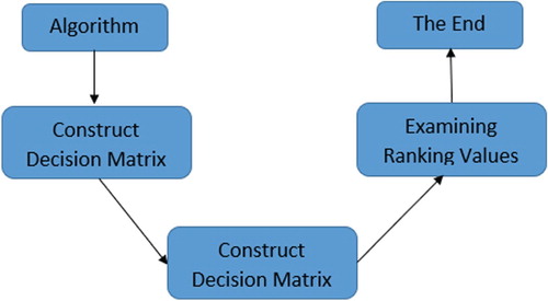
In such a phenomenon, the established SMs are applied to SDM problem. Now, we take the class of an unknown brand strategy and then using the SMs for PHFSs. In such process we evaluate the weighted SMs about the known brands strategies with that of unknown brand strategy. The detail algorithm is the following:

4.4. Algorithm:

1. We take the classes about known and unknown brands strategies in form of PHFNs.

2. Also compute some weighted SMs of each known brands strategies with unknown brand strategy.

3. Discussed the unknown brand strategy based on ranking. The graphical representation of the explored algorithm is discussed in the form of Figure 2.

Figure 2. Geometrical representation of the above algorithm.

Example 1:

Assume that a factory produces a new brand and they are analyzing the optimum targets. The factory divides market in four different strategies such as brand for rich customers, brand for mid-level customers, brand for low-level customers and brand adopted for all customers represented by $Z_i\left(1\le i\le 4\right)$. After this, the DMs have summarised the data of the strategies in five different types such as benefits in long time, benefits in mid time, benefits in short time, risk of the brand strategy and potential market represented by $X=\left\{x_i,i=1,2,\dots ,5\right\}$. In the following, $W=(0.23,0.15,0.34,0.17,0.11{)}^{\text{T}}$ denote a weighted vector of $X$. Table 1 shows that the information about the unknown and known brand strategies and also all numbers are purely in the form of PHFSs. Now, we applied the established weighted SMs to unknown and known brands strategies provided in Table 1 and the results are discussed in Table 2.

Table 1. Date about unknown and known brands strategies.

$x_1$	$\left(\begin{array}{c}\left\{0.10,0.11,0.18\right\},\\ \left\{0.20,0.33,0.38\right\},\\ \left\{0.10,0.25,0.42\right\}\end{array}\right)$	$\left(\begin{array}{c}\left\{0.11,0.20,0.25\right\},\\ \left\{0.17,0.23,0.32\right\},\\ \left\{0.11,0.12,0.14\right\}\end{array}\right)$	$\left(\begin{array}{c}\left\{0.22,0.28,0.33\right\},\\ \left\{0.23,0.25,0.27\right\},\\ \left\{0.01,0.04,0.05\right\}\end{array}\right)$	$\left(\begin{array}{c}\left\{0.35,0.42,0.47\right\},\\ \left\{0.03,0.13,0.18\right\},\\ \left\{0.0,0.02,0.06\right\}\end{array}\right)$	$\left(\begin{array}{c}\left\{0.14,0.15,0.17\right\},\\ \left\{0.27,\mathrm{0.340.37}\right\},\\ \left\{0.34,0.38,0.40\right\}\end{array}\right)$
$x_2$	$\left(\begin{array}{c}\left\{0.11,0.12,0.13\right\},\\ \left\{0.22,0.32,0.42\right\},\\ \left\{0.31,0.35,0.42\right\}\end{array}\right)$	$\left(\begin{array}{c}\left\{1\right\},\\ \left\{0\right\},\\ \left\{0\right\}\end{array}\right)$	$\left(\begin{array}{c}\left\{0.13,0.16,0.22\right\},\\ \left\{0.20,0.24,0.25\right\},\\ \left\{0.33,0.44,0.51\right\}\end{array}\right)$	$\left(\begin{array}{c}\left\{0.10,0.13,0.15\right\},\\ \left\{0.10,0.15,0.17\right\},\\ \left\{0.14,0.16,0.18\right\}\end{array}\right)$	$\left(\begin{array}{c}\left\{0.17,0.18,0.20\right\},\\ \left\{0.43,0.47,0.51\right\},\\ \left\{0.15,0.17,0.20\right\}\end{array}\right)$
$x_3$	$\left(\begin{array}{c}\left\{0.23,0.43,0.53\right\},\\ \left\{0.0,0.05,0.08\right\},\\ \left\{0.20,\mathrm{0.250.30}\right\}\end{array}\right)$	$\left(\begin{array}{c}\left\{0.15,0.17,0.21\right\},\\ \left\{0.32,0.36,0.42\right\},\\ \left\{0.08,0.10,0.14\right\}\end{array}\right)$	$\left(\begin{array}{c}\left\{1\right\},\\ \left\{0\right\},\\ \left\{0\right\}\end{array}\right)$	$\left(\begin{array}{c}\left\{0.10,.16,0.18\right\},\\ \left\{0.15,0.22,0.30\right\},\\ \left\{0.40,0.43,0.45\right\}\end{array}\right)$	$\left(\begin{array}{c}\left\{0.20,0.22,0.25\right\},\\ \left\{0.15,0.17,0.20\right\},\\ \left\{0.30,0.33,0.35\right\}\end{array}\right)$
$x_4$	$\left(\begin{array}{c}\left\{0.20,0.26,0.30\right\},\\ \left\{0.0,0.10,0.20\right\},\\ \left\{0.18,0.30,0.35\right\}\end{array}\right)$	$\left(\begin{array}{c}\left\{1\right\},\\ \left\{0\right\},\\ \left\{0\right\}\end{array}\right)$	$\left(\begin{array}{c}\left\{0.03,0.11,0.17\right\},\\ \left\{0.54,0.58,0.63\right\},\\ \left\{0.10,\mathrm{0.150.20}\right\}\end{array}\right)$	$\left(\begin{array}{c}\left\{0.10,0.21,0.33\right\},\\ \left\{0.02,0.06,0.12\right\},\\ \left\{0.30,0.35,0.40\right\}\end{array}\right)$	$\left(\begin{array}{c}\left\{1\right\},\\ \left\{0\right\},\\ \left\{0\right\}\end{array}\right)$
$x_5$	$\left(\begin{array}{c}\left\{0.20,0.21,0.28\right\},\\ \left\{0.10,0.13,0.18\right\},\\ \left\{0.20,0.25,0.33\right\}\end{array}\right)$	$\left(\begin{array}{c}\left\{0.19,0.20,0.28\right\},\\ \left\{0.18,0.20,0.24\right\},\\ \left\{0.31,\mathrm{0.370.44}\right\}\end{array}\right)$	$\left(\begin{array}{c}\left\{0.31,0.33,0.36\right\},\\ \left\{0.23,0.27,0.30\right\},\\ \left\{0.01,0.05,0.25\right\}\end{array}\right)$	$\left(\begin{array}{c}\left\{0.42,0.44,0.47\right\},\\ \left\{0.13,0.15,0.18\right\},\\ \left\{0.02,0.05,0.06\right\}\end{array}\right)$	$\left(\begin{array}{c}\left\{0.14,0.16,0.18\right\},\\ \left\{0.30,0.34,0.37\right\},\\ \left\{0.30,\mathrm{0.370.42}\right\}\end{array}\right)$

Table 2. Weighted SMs of Ai with A.

Weighted SMs	$\left(Z,Z_1\right)$	$\left(Z,Z_2\right)$	$\left(Z,Z_3\right)$	$\left(Z,Z_4\right)$
$\text{WPHF}{\text{C}}^1\left(Z,Z_i\right)$	0.28826	0.42894	0.16327	0.23604
$\text{WPHF}{\text{C}}^2\left(Z,Z_i\right)$	0.27855	0.33848	0.17467	0.23195
$\text{WPHFC}{\text{S}}^1\left(Z,Z_i\right)$	0.86721	0.85294	0.58029	0.81388
$\text{WPHFC}{\text{S}}^2\left(Z,Z_i\right)$	0.90551	0.88067	0.67253	0.84847
$\text{WPHFC}{\text{S}}^3\left(Z,Z_i\right)$	0.85917	0.84482	0.58029	0.80435
$\text{WPHFC}{\text{S}}^4\left(Z,Z_i\right)$	0.83075	0.82753	0.55644	0.72663
$\text{WPHFC}{\text{T}}^1\left(Z,Z_i\right)$	0.67166	0.67480	0.37498	0.59880
$\text{WPHFC}{\text{T}}^2\left(Z,Z_i\right)$	0.64823	0.66124	0.37498	0.58503

Step 1: Class of unknown and known brands strategies.

Step 2: Comparison of some weighted SMs.

Step 3: We consider the weight of $x_i\left(i=0.23,0.15,0.34,0.17and0.11\right),$ respectively. Then we evaluate the weighted SMs about the class of unknown and known brands strategies. After evaluation we see that in Table 2, the SM of $\left(Z,Z_2\right)$ is greater among all other SMs by using cosine SM for PHFSs and SMs for PHFSs based on cotangent function. But on the other hand SMs of $\left(Z,Z_1\right)$ have larger value of SMs among all other SMs by using the SMs for PHFSs based on cosine function. Therefore, it is clear that the SMs give us different results by using different approaches.

5. Comparative Study

The aim of this section is to establish the comparative study of the proposed work with existing SMs. The proposed SMs are compared with some cosine SMs for PFS was introduced by Wei [36], SMs for spherical fuzzy sets based on cosine function was introduced by Wei et al. [43], SMs for T-spherical fuzzy sets based on cosine function was introduced by Mahmood et al. [45], and improve cosine SMs of simplified neutrosophic sets was introduced by Ye [46].

Example 2:

In this example, we take PFS type’s framework and show that the comparison of the proposed works with existing SMs. For this, we assume that a factory produces a new brand and they are analyzing the optimum targets. The factory divides market in four different strategies such as brand for rich customers, brand for mid-level customers, brand for low-level customers and brand adopted for all customers represented by $Z_i\left(1\le i\le 4\right)$. After this, the DMs have summarised the data of the strategies in five different types such as benefits in long time, benefits in mid time, benefits in short time, risk of the brand strategy and potential market represented by $X=\left\{x_i,i=1,2,\dots ,5\right\}$. In the following, $W=(0.23,0.15,0.34,0.17,0.11{)}^{\text{T}}$ denote a weighted vector of $X$. Table 3 shows that the information about the unknown and known brand strategies.

Table 3. Date about unknown and known brands strategies.

	$Z_1$	$Z_2$	$Z_3$	$Z_4$	$Z$
$x_1$	$\left(0.42,0.35,0.18\right)$	$\left(0.03,0.82,0.13\right)$	$\left(0.04,0.85,0.10\right)$	$\left(0.02,0.89,0.05\right)$	$\left(0.05,0.87,0.06\right)$
$x_2$	$\left(0.10,0.81,0.05\right)$	$\left(0.62,0.12,0.07\right)$	$\left(0.60,0.26,0.11\right)$	$\left(1,0,0\right)$	$\left(0.78,0.12,0.07\right)$
$x_3$	$\left(0.33,0.51,0.12\right)$	$\left(1,0,0\right)$	$\left(0.15,0.76,0.07\right)$	$\left(0.16,0.71,0.05\right)$	$\left(0.15,0.73,0.08\right)$
$x_4$	$\left(0.89,0.08,0.03\right)$	$\left(0.13,0.64,0.21\right)$	$\left(1,0,0\right)$	$\left(0.74,0.16,0.10\right)$	$\left(0.68,0.08,0.21\right)$
$x_5$	$\left(0.08,0.89,0.02\right)$	$\left(0.73,0.15,0.08\right)$	$\left(0.68,0.26,0.06\right)$	$\left(0.08,0.84,0.06\right)$	$\left(0.13,0.75,0.09\right)$

Step 1: The class about unknown and known brands strategies.

The comparison of the proposed work with the existing drawback is discussed in example 2 and expressed as in Table 4.

Table 4. Comparison of the proposed work with existing drawback.

Methods	SMs	Ranking
Wei [36]	$\text{S}{\text{M}}_{\text{PFS}}\left(Z,Z_1\right)$=0.8201,$\text{S}{\text{M}}_{\text{PFS}}\left(Z,Z_2\right)$=0.6402$\text{S}{\text{M}}_{\text{PFS}}\left(Z,Z_3\right)$=0.9377,$\text{S}{\text{M}}_{\text{PFS}}\left(Z,Z_4\right)$=0.9874	$Z_4>Z_3>Z_1>Z_2$
Wei et al. [43]	$\text{S}{\text{M}}_{\text{PFS}}\left(Z,Z_1\right)$=0.8627,$\text{S}{\text{M}}_{\text{PFS}}\left(Z,Z_2\right)$=0.7105$\text{S}{\text{M}}_{\text{PFS}}\left(Z,Z_3\right)$=0.9485,$\text{S}{\text{M}}_{\text{PFS}}\left(Z,Z_4\right)$=0.9902	$Z_4>Z_3>Z_1>Z_2$
Mahmood et al. [45]	$\text{S}{\text{M}}_{\text{PFS}}\left(Z,Z_1\right)$=0.9024,$\text{S}{\text{M}}_{\text{PFS}}\left(Z,Z_2\right)$=0.7758$\text{S}{\text{M}}_{\text{PFS}}\left(Z,Z_3\right)$=0.9543,$\text{S}{\text{M}}_{\text{PFS}}\left(Z,Z_4\right)$=0.9855	$Z_4>Z_3>Z_1>Z_2$
Ye [46]	$\text{S}{\text{M}}_{\text{PFS}}\left(Z,Z_1\right)$=0.9170, $\text{S}{\text{M}}_{\text{PFS}}(Z,Z_2{)}_{}$=0.8289$\text{S}{\text{M}}_{\text{PFS}}\left(Z,Z_3\right)$=0.9717,$\text{S}{\text{M}}_{\text{PFS}}\left(Z,Z_4\right)$=0.9944	$Z_4>Z_3>Z_1>Z_2$
$\text{WPHFC}{\text{S}}^2\left(Z,Z_i\right)$	$\text{S}{\text{M}}_{\text{PFS}}\left(Z,Z_1\right)$=0.8201,$\text{S}{\text{M}}_{\text{PFS}}\left(Z,Z_2\right)$=0.6402$\text{S}{\text{M}}_{\text{PFS}}\left(Z,Z_3\right)$=0.9377,$\text{S}{\text{M}}_{\text{PFS}}\left(Z,Z_4\right)$=0.9874	$Z_4>Z_3>Z_1>Z_2$

Step 2: Comparison of some SMs.

After evaluation in Table 4, we see that the SM of $\left(Z,Z_4\right)$ is greater among all other SMs.

Finally, the comparison of the established work with the existing drawback is discussed in example 1 and expressed as in Table 5.

Table 5. Comparison of the proposed work with existing drawback.

Methods	SMs	Ranking
Wei [36]	$\text{Cannot be classified}$	$\text{Cannot be classified}$
Wei et al. [43]	$\text{Cannot be classified}$	$\text{Cannot be classified}$
Mahmood et al. [45]	$\text{Cannot be classified}$	$\text{Cannot be classified}$
Ye [46]	$\text{Cannot be classified}$	$\text{Cannot be classified}$
$\text{WPHFC}{\text{S}}^2\left(Z,Z_i\right)$	$\text{S}{\text{M}}_{\text{PFS}}\left(Z,Z_1\right)$=0.90551,$\text{S}{\text{M}}_{\text{PFS}}\left(Z,Z_2\right)$=0.88067$\text{S}{\text{M}}_{\text{PFS}}\left(Z,Z_3\right)$=0.67253,$\text{S}{\text{M}}_{\text{PFS}}\left(Z,Z_4\right)$=0.84847	$Z_1>Z_2>Z_4>Z_3$

Analyzing Tables 4 and 5, it is clear that, the proposed SMs are the generalisation of SMs for PFSs, SMs for spherical fuzzy sets based on cosine function, SMs for T-spherical fuzzy sets based on cosine function and improved cosine SMs for simplified neutrosophic sets. Therefore, it shows that, the established SMs are more reliable and general than existing notions due to its conditions. Because if we take PHFS types information, the existing SMs is not able to solve it, but when we take PFS types of data like in example 2, the proposed work can easily solve. Hence, it is clear that the established SMs will become the special case of the existing SMs.

5.1. Advantages

• Due to some limitation of SMs in References [34,36], we introduced some new SMs for PHFSs. Further, we show that the existing SMs could not be handling the information like in example 2.

• The main advantage of the proposed SMs is that, these SMs can easily solve the problems of the previous SMs defined so far in References [34,36].

• The SMs in References [34,36] will become the special of the proposed SMs. Therefore, the proposed SMs are more reliable and suitable to solve the real-life problem.

5.2. Limitations

The notion of PHFS is the mixture of two different notion are called PFS and hesitant fuzzy set to cope with uncertain and unpredictable information’s in realistic decision issues. PHFS is contains the grade of truth, abstinence and falsity with the condition that is the sum of the maximum of the truth, abstinence and falsity grades is cannot exceed from unit interval. PHFS is more reliable then PFSPFS, intuitionistic fuzzy set, fuzzy set and hesitant fuzzy set, because these all are the special cases of the presented works.

6. Conclusion

PHFS is a mixture of PFS and hesitant fuzzy set to cope with awkward and difficult information in realistic decision issues. The PFS and hesitant fuzzy set are the special cases of the PHFS. Keeping the advantages of the PHFS, in this article, we proposed the similarity measures for PHFSs based on cosine function, including cosine similarity measures for PHFSs, similarity measures for PHFS s based on cosine function and similarity measures for PHFSs based on cotangent function. Further, we introduced some weighted similarity measures and also described that the conditions under which, similarity measures for PHFSs reduced to similarity measures for IHFSs. Then, the weighted similarity measures are applied to strategic decision-making problem and the results are discussed. Moreover, we compare the established work with existing drawback and also identify that the existing drawback cannot solve the problem of established work. But on the other hand, the new approach can easily solve the problem of the existing drawback.

In the future work, we will apply the established work to some other areas like interval-valued PHFS, group decision-making problem, medical diagnosis and many other fields [37,38,46–48].

Disclosure statement

No potential conflict of interest was reported by the author(s).

Additional information

Notes on contributors

Tahir Mahmood

Tahir Mahmood is Assistant Professor of Mathematics at Department of Mathematics and Statistics, International Islamic University Islamabad, Pakistan. He received his Ph.D. degree in Mathematics from Quaid-i-Azam University Islamabad, Pakistan in 2012 under the supervision of Professor Dr. Muhammad Shabir. His areas of interest are Algebraic structures, Fuzzy Algebraic structures, and Soft sets. He has more than 160 international publications to his credit and he has also produced more than 45 MS students and 6 PhD students.

Zeeshan Ahmad

Zeeshan Ahmad, received his master’s degree in Mathematics from International Islamic University Islamabad, Pakistan, in 2018. His research interests include aggregation operators, fuzzy logic, fuzzy decision making, and their applications. He has published 4 articles in well reputed journals.

Zeeshan Ali

Zeeshan Ali, received the B.S. degrees in Mathematics from Abdul Wali Khan University Mardan, Pakistan, in 2016. He received has M.S. degrees in Mathematics from International Islamic University Islamabad, Pakistan, in 2018. Currently, He is a Student of Ph. D in mathematics from International Islamic University Islamabad, Pakistan. His research interests include aggregation operators, fuzzy logic, fuzzy decision making, and their applications. He has published more than forty articles in reputed journals.

Kifayat Ullah

Kifayat Ullah is working as Assistant Professor of Mathematics at the Department of Mathematics, Riphah Institute Computing and Applied Sciences, Riphah International University Lahore, Pakistan. He received his Ph.D. degree in Mathematics from International Islamic University Islamabad, Pakistan in 2020. He also worked as research fellow the Department of Data Analysis and Mathematical Modeling at Ghent University Belgium. His areas of interest include fuzzy aggregation operators, information measures, fuzzy relations, fuzzy graph theory and soft set theory. He has more than 30 international publications to his credit.

References

- Zadeh LA. Fuzzy sets. Information and Control. 1965;8:338–353.
- Atanassov KT. Intuitionistic fuzzy sets. Fuzzy Sets and Systems. 1986;20(1):87–96.
- Atanassov KT. More on intuitionistic fuzzy sets. Fuzzy Sets and Systems. 1989;33(1):37–45.
- Yazdanbakhsh O, Dick S. A systematic review of complex fuzzy sets and logic. Fuzzy Sets and Systems. 2018;338:1–22.
- Asiain MJ, et al. Negations with respect to admissible orders in the interval-valued fuzzy set theory. IEEE Transactions on Fuzzy Systems. 2018;26(2):556–568.
- Jan N, Ullah K, Mahmood T, et al. Some root level modifications in interval valued fuzzy graphs and their generalizations including neutrosophic graphs. Mathematics. 2019;7(1):72.
- Kumar K, Garg H. Connection number of set pair analysis based TOPSIS method on intuitionistic fuzzy sets and their application to decision making. Applied Intelligence. 2018;48(8):2112–2119.
- Garg H, Kumar K. Some aggregation operators for linguistic intuitionistic fuzzy set and its application to group decision-making process using the set pair analysis. Arabian Journal for Science and Engineering. 2018;43(6):3213–3227.
- Mahmood T, et al. Several hybrid aggregation operators for triangular intuitionistic fuzzy set and their application in multi-criteria decision making. Granular Computing. 2018;3(2):153–168.
- Kim T, Sotirova E, Shannon A, et al. Interval valued intuitionistic fuzzy evaluations for analysis of a student’s knowledge in university e-learning courses. International Journal of Fuzzy Logic and Intelligent Systems. 2018;18(3):190–195.
- Cuong BC. Picture fuzzy sets. Journal of Computer Science and Cybernetics. 2014;30(4):409–420.
- Singh P. Correlation coefficients for picture fuzzy sets. Journal of Intelligent & Fuzzy Systems. 2015;28(2):591–604.
- Garg H. Some picture fuzzy aggregation operators and their applications to multi-criteria decision-making. Arabian Journal for Science and Engineering. 2017;42(12):5275–5290.
- Wei G. Picture fuzzy aggregation operators and their application to multiple attribute decision making. Journal of Intelligent & Fuzzy Systems. 2017;33(2):713–724.
- Wei G. Picture fuzzy Hamacher aggregation operators and their application to multiple attribute decision making. Fundamental Informatica. 2018;157(3):271–320.
- Torra V. Hesitant fuzzy sets. International Journal of Intelligent Systems. 2010;25(6):529–539.
- Beg I, Rashid T. Group decision making using intuitionistic hesitant fuzzy sets. International Journal of Fuzzy Logic and Intelligent Systems. 2014;14(3):181–187.
- Mahmood T, Mahmood F, Khan Q. Some generalized aggregation operators for cubic hesitant fuzzy sets and their applications to multi criteria decision making. Journal of Mathematics. 2017: 1016–2526. 49(1), 31-49.
- Ullah K, Mahmood T, Jan N, et al. On bipolar-valued hesitant fuzzy sets and their applications in multi-attribute decision making. The Nucleus. 2018;55(2):93–101.
- Farhadinia B. Information measures for hesitant fuzzy sets and interval-valued hesitant fuzzy sets. Inf Sci (Ny). 2013;240:129–144.
- Zhai Y, Xu Z, Liao H. Measures of probabilistic interval-valued intuitionistic hesitant fuzzy sets and the application in reducing excessive medical examinations. IEEE Transactions on Fuzzy Systems. 2017;26(3):1651–1670.
- Mahmood T, Ullah K, Khan Q, et al. Some aggregation operators for bipolar-valued hesitant fuzzy information. Journal of Fundamental and Applied Sciences. 2018;10(4S):240–245.
- Deli I. A TOPSIS method by using generalized trapezoidal hesitant fuzzy numbers and application to a robot selection problem. Journal of Intelligent & Fuzzy Systems. 2020;38(1):779–793.
- Akram M, Ali G, Alcantud JCR. New decision-making hybrid model: intuitionistic fuzzy N-soft rough sets. Soft Comput. 2019;23(20):9853–9868.
- Akram M, Ali G. Hybrid models for decision-making based on rough Pythagorean fuzzy bipolar soft information. Granular Computing. 2020;5(1):1–15.
- Akram M, Ali G, Waseem N, et al. Decision-making methods based on hybrid mF models. Journal of Intelligent & Fuzzy Systems. 2018;35(3):3387–3403.
- Wang R, Li Y. Picture hesitant fuzzy set and its application to multiple criteria decision-making. Symmetry (Basel). 2018;10(7):295. https://doi.org/10.3390/sym10070295.
- Hesamian G, Chachi J. On Similarity Measures for fuzzy sets with applications to pattern recognition, decision making, clustering, and approximate reasoning. Journal of Uncertain Systems. 2017;11(1):35–48.
- Lohrmann C, Luukka P, Jablonska-Sabuka M, et al. A combination of fuzzy Similarity Measures and fuzzy entropy measures for supervised feature selection. Expert Syst Appl. 2018;110:216–236.
- Dhavudh SS, Srinivasan R. Intuitionistic fuzzy graphs of second type. Advances in Fuzzy Mathematics. 2017;12(2):197–204.
- Hwang CM, Yang MS, Hung WL. New Similarity Measures of intuitionistic fuzzy sets based on the Jaccard index with its application to clustering. International Journal of Intelligent Systems. 2018;33(8):1672–1688.
- Song Y, Wang X, Quan W, et al. A new approach to construct SM for intuitionistic fuzzy sets. Soft Comput. 2019;23(6):1985–1998.
- Li Y, Olson DL, Qin Z. Similarity Measures between intuitionistic fuzzy (vague) sets: A comparative analysis. Pattern Recognit Lett. 2007;28(2):278–285.
- Ye J. Similarity Measures of intuitionistic fuzzy sets based on cosine function for the decision making of mechanical design schemes. Journal of Intelligent & Fuzzy Systems. 2016;30(1):151–158.
- Wei G. Some Similarity Measures for picture fuzzy sets and their applications. Iranian Journal of Fuzzy Systems. 2018;15(1):77–89.
- Wei G. Some cosine Similarity Measures for picture fuzzy sets and their applications to strategic decision making. Informatica. 2017;28(3):547–564.
- Thao NX. Similarity Measures of picture fuzzy sets based on entropy and their application in MCDM. Pattern Analysis and Applications. 2019;23(3):1203–1213.
- Zhang Y, Wang L, Yu X, et al. A new concept of cosine Similarity Measures based on dual hesitant fuzzy sets and its possible applications. Cluster Comput. 2018;22(6):15483–15492.
- Zhang Z, Li J, Sun Y, et al. Novel distance and Similarity Measures on hesitant fuzzy linguistic term sets and their application in clustering analysis. IEEE Access. 2019;7:100231–100242.
- Ullah K, Mahmood T, Jan N. Similarity Measures for T-spherical fuzzy sets with applications in pattern recognition. Symmetry (Basel). 2018;10(6):193. https://doi.org/10.3390/sym10060193.
- Wang P, Wang J, Wei G, et al. Similarity Measures of q-rung orthopair fuzzy sets based on cosine function and their applications. Mathematics. 2019;7(4):340. https://doi.org/10.3390/math7040340.
- Wei G, Wei Y. Similarity Measures of Pythagorean fuzzy sets based on the cosine function and their applications. International Journal of Intelligent Systems. 2018;33(3):634–652.
- Wei G, Lu J, Wang J, et al. Similarity Measures of spherical fuzzy sets based on cosine function and their applications. IEEE Access. 2019;7:159069–159080.
- Ahmad Z, Mahmood T, Saad M, et al. Similarity Measures for picture hesitant fuzzy sets and their applications in pattern recognition. Journal of Prime Research in Mathematics. 2019;15:81–100.
- Mahmood T, Ahmad Z, Garg H, et al. Similarity Measures for T-spherical fuzzy sets based on cosine function and their applications. Journal of complex and intelligent systems. 2020.
- Ye J. Improved cosine Similarity Measures of simplified neutrosophic sets for medical diagnoses. Artificial Intelligence in Medicine. 2015;63(3):171–179.
- Liu P, Ali Z, Mahmood T. A method to multi-attribute group decision-making problem with Complex q-rung orthopair linguistic information based on Heronian mean operators. International Journal of Computational Intelligence Systems. 2019;12(2):1465–1496.
- Liu P, Mahmood T, Ali Z. Complex q-rung orthopair fuzzy aggregation operators and their applications in multi-attribute group decision making. Information. 2020;11(1):5. https://doi.org/10.3390/info11010005.