
 ?Mathematical formulae have been encoded as MathML and are displayed in this HTML version using MathJax in order to improve their display. Uncheck the box to turn MathJax off. This feature requires Javascript. Click on a formula to zoom.
Abstract
In this article, we try to solve a full fuzzy algebraic equation with a fuzzy variable and fuzzy coefficients. This can be done by a numerical iterative process. We offer an algorithm to produce a sequence that may converge to a root of such an equation.
1. Introduction
In many purposes of a system, we may need to solve a fuzzy equation. Zadeh introduced some properties of fuzzy equations in [Citation1] and some other types of such equations were discussed by some researchers [Citation2, Citation3] and they tried to solve them analytically. Solving an algebraic equation of degree at most 3 has no analytical method even in crisp form. So it is necessary to find the numerical solution of an equation. In [Citation4], fuzzy nonlinear equations with fuzzy unknown were considered. A research effort has been done on algebraic fuzzy equations by using neural network [Citation5]. Two numerical iterative methods have been presented in [Citation6, Citation7] to find the roots of an algebraic fuzzy equation of degree n, one with fuzzy coefficients and crisp unknown and the other one with crisp coefficients and fuzzy unknown. In the present essay, we introduce a numerical method to solve a full fuzzy algebraic equation, such that all numbers are fuzzy, both the unknown variable and coefficients. The organisation of the present paper is as follows. In Section 2, we represent a full fuzzy algebraic equation and we discuss solving a nonlinear system of equations. In Section 3, an algorithm is introduced to numerically solving a full fuzzy algebraic fuzzy equation. Some examples are given in Section 4, and Section 5 contains the conclusion of this work.
2. Preliminaries
The presentation of a fuzzy number by a pair of functions as
is called the parametric form of
, such that over
, we have:
is a left continuous and monotonically increasing function,
is a left continuous and monotonically decreasing function, and
[Citation8–12]. We consider the set of all fuzzy numbers by
.
Suppose and
are both belonging to
. Then some operations are defined as follows:
;
If
A fuzzy number is called non-negative (non-positive) if
on
. Also
is called positive (negative), if
on
. It is obvious that for non-negative fuzzy numbers
and
we have
, and for non-positive fuzzy numbers
and
we have
.
Definition 2.1
cut of a fuzzy number
is the interval
, and we use the notation
for it.
Definition 2.2
is a fuzzy polynomial of degree at most n with fuzzy coefficients, if there are some fuzzy numbers
, such that
(1)
(1)
For a positive integer n, an algebraic equation with full fuzzy feature of degree n, can be defined as
(2)
(2)
where
,
and
.
Definition 2.3
A ‘m-degree polynomial form’ fuzzy number is defined by a pair
, such that
and
are two polynomials of degree at most m [Citation13–15].
We use for the set of all m-degree polynomial form fuzzy numbers [Citation13, Citation14, Citation16]. Let
be a function such that maps
to
, where
. To solve the system of equations
(3)
(3)
by Gauss–Newton method [Citation17], we consider
as the Jacobian of F:
,
and
. Considering
as an initial vector, we try to improve this guess, so the system
should be solved in each iteration and then the approximated solution will be improved by considering
. This system of equation can be solved by a least square method as the following:
(4)
(4)
Some conditions on convergence and uniqueness of the solution of (Equation3
(3)
(3) ) are proposed [Citation18–20]. Let
and
for
are known fuzzy numbers. We try to solve the following full fuzzy algebraic equation from degree n:
(5)
(5)
in which we have
. We consider
as the unknown fuzzy root of Equation (Equation5
(5)
(5) ).
3. Solving the Algebraic Fuzzy Equation
Let the unknown be a fuzzy number belonging to
. Also let we have
and
, in which
. We discuss about Equation (Equation5
(5)
(5) ), by four cases:
First we consider the case that the unknown fuzzy number
Let
In the case that
If
In the last three cases, rewriting the equations by an ordering on the power of r leads us to introduce two functions and
for
, which are the coefficients of
(
respect to (Equation14
(14)
(14) ), (Equation16
(16)
(16) ) or (Equation18
(18)
(18) ) and
respect to (Equation15
(15)
(15) ), (Equation17
(17)
(17) ) or (Equation19
(19)
(19) )). For
both functions
and
are functions of
's and
's. Thus we have
(20)
(20)
and
(21)
(21)
Let us introduce two functions
and
as follows:
(22)
(22)
and
(23)
(23)
Therefore we have
(24)
(24)
Equation (Equation24
(24)
(24) ) is a nonlinear system of equations with
equations and s = 2k + 2 unknowns, so it can be solved by an iterative Gauss–Newton method. Suppose that t = nk + m Defining
(25)
(25)
and
(26)
(26)
we have
(27)
(27)
A and B are used instead of
and
, respectively. By solving this system with an initial vector
, a sequence
will be obtained as follows: we consider an initial vector
. For
, we compute
and
and then we solve
by a least square method:
(28)
(28)
and the obtaining vector will be improved by
(29)
(29)
Again
and
are used instead of
and
, respectively. If
converges to a vector
; then
is a solution of (Equation5
(5)
(5) ) where
(30)
(30)
Therefore the algorithm will be as follows:
Lemma 3.1
If the fuzzy Equation (Equation5(5)
(5) ) has a root
then
is a root of the equation
Corollary 3.2
The algebraic fuzzy equation of degree n (Equation5(5)
(5) ) has at most n fuzzy roots with distinct cores.
Theorem 3.3
If the equation is crisp then the sequence is given by the following recurrence equation:
(31)
(31)
Proof.
For a crisp function algebraic equation , we have
and
, where
. For this equation, we have
(32)
(32)
The system (Equation27
(27)
(27) ) for this equation is as follows:
Using
, we have
, and
, therefore in the iteration
, we have
.
By using the following lemma, we find that Algorithm 3.1 always generate a sequence.
Lemma 3.4
[Citation21]
The system (Equation28(28)
(28) ) always has a solution, for any k.
4. Numerical Examples
In this section, we present some examples of full fuzzy algebraic equations. All examples are solved by commercial software Mathematica 10.
Example 4.1
Consider the following equation:
such that
For this equation, we have n = 2, l = 3 and m = 1. The least acceptable value of k is 1. By considering k = 1 and the initial fuzzy number
, after 6 iterations and 12 digits accuracy, we obtain
. In this case,
is the solution of
.
Example 4.2
For equation:
with
we have n = 2, l = 5 and m = 1. The least acceptable value of k is 2. By considering k = 2 and the initial fuzzy number
, after 6 iterations and 11 digits accuracy, we obtain
. In this case,
is the solution of
.
Example 4.3
Consider the following equation:
such that
For this equation, we have n = 2, l = 3 and m = 1 and one of the coefficients is non-positive. The least acceptable value of k is 1. By considering k = 1 and the initial fuzzy number
, after 7 iterations and 8 digits accuracy, we obtain
. In this case,
is the solution of
.
Example 4.4
Consider the following equation:
such that
For this equation, we have n = 2, l = 3 and m = 1. The least acceptable value of k is 1. By considering k = 1 and the initial fuzzy number
, after 7 iterations and 8 digits accuracy, we obtain
. In this case,
is the solution of
. Here the root of equation is non-positive.
Example 4.5
For the following equation:
with
we have n = 2, l = 3 and m = 1 and one of the coefficients is negative. The least acceptable value of k is 1. By considering k = 1 and the initial fuzzy number
, after 8 iterations and 8 digits accuracy, we obtain
. In this case,
is the solution of
. Here the root of equation is non-positive.
Example 4.6
Suppose that we want to solve the following equation:
For this equation, we have n = 4, l = 5 and m = 1. The least acceptable value of k is 1. By considering k = 1 and the initial fuzzy number
, after 10 iterations we obtain
. In this case,
is the solution of
.
Example 4.7
Suppose that a car is moving in a straight line with the velocity . If this car breaks, after a time
it will stop. The distance satisfies in the following relation:
(33)
(33)
in which
is the constant negative acceleration and
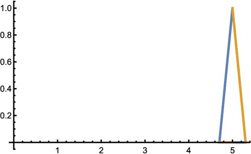
is the stopping time, and all variables are linguistic (Figure ). If acceleration is about
and the velocity is about
, then by solving the equation, it will be clear that the car will stop after about 5 s (Figures and ).
Figure 1. The time of breaking.
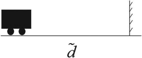
Figure 2. The coefficients of quadratic equation: (a) Velocity, (b) Acceleration and (c) Distance.
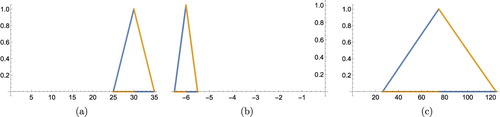
Figure 3. Stopping time.
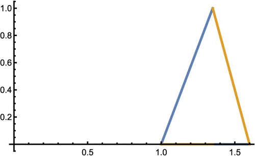
Example 4.8
Consider the following fuzzy linear differential equation of order n:
where
is the independent crisp variable. In order to find the solution of this ODE one must solve the following fuzzy algebraic equation of degree n:
For example by considering
and
as shown in Figure , the solution of quadratic equation is the fuzzy number which is shown in Figure and the solution of related differential equation is
(Figures and ).
Figure 4. The coefficients of quadratic equation: (a) , (b)
and (c)
.
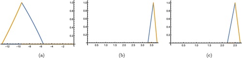
Figure 5. Root of equation.
5. Conclusion
In this work, we presented a method to find a numerical solution of a full fuzzy algebraic equation. The method can be used for any kind of fuzzy equations, with non-positive or non-negative roots and with non-positive or non-negative coefficients. Some possible future research directions may consist of the more general case than the four cases which considered in this paper, and using the proposed for multiple roots of an equation.
Disclosure statement
No potential conflict of interest was reported by the authors.
Additional information
Notes on contributors
Majid Amirfakhrian
Majid Amirfakhrian was born and raised in Tehran, Iran. He went to the University of Guilan, Rasht, Iran for his post–secondary education. He received his Master of Science in Applied Mathematics from the Sharif University of Technology and completed his Ph.D. through the Azad University, Science and Research branch. He joined the Azad University, Central Tehran Branch (IAUCTB) in 2002. He was promoted to a full professorship of Applied Mathematics at IAUCTB in 2015. His main research interests lie in Numerical Analysis and Approximation, Fuzzy Approximation, Data Sciences, Multivariate Approximation, Image Processing, and Numerical Partial Differential Equations. He has side interests in Optimization and Statistics.
S. R. Fayyaz Behrooz
S. R. Fayyaz Behrooz was born on November 22, 1978, and grown up in Tabriz, Iran. She received an M.S. degree from Tabriz University in 2004 and a B.S. degree from Islamic Azad University, Tabriz Branch in 2002. She is currently a Ph.D. student at the Islamic Azad University, Central Tehran Branch, Iran. She is a faculty member at Islamic Azad University, Osku Branch since 2008. Her main research interest includes Numerical and Computational Methods in Science and Fuzzy problems.
References
- Zadeh LA. Toward a generalized theory of uncertainty (GTU) an outline. Inform Sci. 2005;172:1–40.
- Buckley JJ, Qu Y. Solving linear and quadratic fuzzy equations. Fuzzy Sets Syst. 1990;38:43–59.
- Zhao R, Govind R. Solutions of algebraic equations involving generalized fuzzy numbers. Inform Sci. 1991;56:199–243.
- Abbasbandy S, Asady B. Newton's method for solving fuzzy nonlinear equations. Appl Math Comput. 2004;159:349–356.
- Abbasbandy S, Otadi M. Numerical solution of fuzzy polynomials by a fuzzy neural network. Appl Math Comput. 2006;181:1084–1089.
- Amirfakhrian M. Numerical solution of algebraic fuzzy equations with crisp variable by Gauss–Newton method. Appl Math Model. 2008;32:1859–1868.
- Amirfakhrian M. An iterative Gauss–Newton method to solve an algebraic fuzzy equation with crisp coefficients. J Intel Fuzzy Syst. 2011;22:207–216.
- Friedman M, Ma M, Kandel A. Fuzzy linear systems. Fuzzy Sets Syst. 1998;96:201–209.
- Ma M, Friedman M, Kandel A. A new fuzzy arithmetic. Fuzzy Sets Syst. 1999;108:83–90.
- Ma M, Kandel A, Friedman M. A new approach for defuzzification. Fuzzy Sets Syst. 2000;111:351–356.
- Stefanini L, Sorini L, Guerra ML. Parametric representation of fuzzy numbers and application to fuzzy calculus. Fuzzy Sets Syst. 2006;157:2423–2455.
- Goestschel R, Voxman W. Elementary calculus. Fuzzy Sets Syst. 1986;18:31–43.
- Abbasbandy S, Amirfakhrian M. The nearest approximation of a fuzzy quantity in parametric form. Appl Math Comput. 2006;172:624–632.
- Abbasbandy S, Amirfakhrian M. The nearest trapezoidal form of a generalized left right fuzzy number. Int J Approx Reason. 2006;43:166–178.
- Amirfakhrian M. Some approximation methods in fuzzy logic: some method for finding approximation of fuzzy functions and fuzzy numbers. Germany: Lambert Academic Publishing; 2012.
- Amirfakhrian M. Numerical solution of a system of polynomial parametric form fuzzy linear equations. Chapter 24, in Book ‘Ferroelectrics’, INTECH Publisher; 2010.
- Deuflhard P. Newton methods for nonlinear problems. Berlin: Springer-Verlag Berlin Heidelberg; 2004.
- Chen J, Li W. Convergence of Gauss–Newton's method and uniqueness of the solution. Appl Math Comput. 2005;170:686–705.
- Chen J, Li W. Local convergence results of Gauss–Newton's like method in weak conditions. J Math Anal Appl. 2006;324:1381–1394.
- Li C, Zhang WH, Jin XQ. Convergence and uniqueness properties of Gauss–Newton's method. Comput Math Appl. 2004;47(6–7):1057–1067.
- Gill PE, Murray W, Wright MH. Numerical linear algebra and optimization. Redwood City (CA): Addison–Wesley Publishing Company; 1991.