Agriculture Crop Suitability Prediction Using Rough Set on Intuitionistic Fuzzy Approximation Space and Neural Network

Abstract

Agriculture plays a vital role in Indian economy. On considering the overall geographical space verses population in India, 7% of population is chronicled in Tamilnadu, with 3% of water and 4% of land resources. Thus an automated prediction system becomes essential for predicting the crop based on the nutritional security of the country. In this paper, effort has been made to process the uncertainties by hybridizing rough set on intuitionistic fuzzy approximation space (RSIFAS) [Acharjya DP, Tripathy BK. Rough sets on intuitionistic fuzzy approximation spaces and knowledge representation. Int J Artif Int Comput Res. 2009;1 (1):29–36.] and neural network [Hecht NR. Theory of the backpropagation neural network. Proceedings of the international Joint Conference on neural networks, 1 (1989), 593–605.]. RSIFAS identifies the almost indiscernibility among the natural resources, and helps in reducing the computational procedure on employing data reduction techniques whereas neural network helps in prediction process. It helps to find the crops that may be cultivated based on the available natural resources. The proposed model is analyzed on data accumulated from Vellore district of Tamilnadu, India and achieved 93.7% of average classification accuracy. The model is compared with earlier models and found 6.9% better accuracy while prediction.

KEYWORDS:

• Almost indiscernible
• intuitionistic fuzzy proximity relation
• neural network
• knowledge discovery
• prediction
• rough set

1. Introduction

In India, for over 58.4% of its population, agriculture is the principal means of livelihood. In addition, the agricultural merchandises are considered as the main commodity for the international trading. To sustain the growth of the Indian economy, there is a need for a drastic growth in agriculture productivity. For agriculture, the land and water are the main resources, which are inadequate in nature. Consequently, it is necessary to devise a lucrative cropping system with the accessible resources and to increase the productivity. Ever since, the market competition is high, a premeditated planning is mandatory to improve the performance to accomplish a profitable yield in the cropping system. The perfect planning in the development and production of the cropping system may step back due to uncertainty in forecasting the harvesting and demand for the crop. Therefore, to investigate the information for future planning can be achieved by a prediction model. A prediction model developed with the prior knowledge gives more accuracy towards the real-life situations. Thus, the proposed prediction model is based on soil and water resources available in some region to forecast the production of agricultural crops, with reduced risk of loss. Due to the lack of natural and human resources, many farmers agree themselves to alter the agriculture land into marketable land. This attitude has to be changed so as to retain the farmers and especially young generation to take up agriculture as their main occupation, and the income from the farm holding should be amplified significantly.

The area of study of this paper restricted to Vellore district in Tamil Nadu where agriculture is the main vocation. The small and marginal farmers in this region play a key role in the overall improvement in agriculture towards the development of the Indian economy. Thus, the adoption of appropriate cropping system by these farmers needs to be focused. Indian government has taken some productivity measure to improve the crop production by: training the farmers, relaxing the seed cost and loan amount etc. To tackle the increasing competency, it becomes more essential to develop a crop suitability information system to improve the productivity, and profit for the farmers. To develop such an effective system, data collected from various sources such as soil, water, seedling methodologies and meteorological conditions must be analysed properly instead of saving as archives.

Analysing data and discovering knowledge is a challenging and increasingly important task as it contains uncertainties. Additionally, it is not always useful to users as it may not certainly satisfy user’s choice due to the presence of redundancy, inconsistency and vagueness. Many traditional tools used for discovering knowledge are deterministic, crisp and precise. Thus, it is essential to use some intelligent techniques so as to process the uncertainties present in the data. The emergence of intelligent computing techniques like fuzzy set [1], rough set [2,3], rough set on fuzzy approximation space (RSFAS) [4,5], rough set on intuitionistic fuzzy approximation space (RSIFAS) [6], soft set [7], near set [8], fuzzy rough set [9], rough set on two universal sets [10], neutrosophic set [11] etc. plays a vital role in knowledge discovery. Further, RSFAS is hybridised with Bayesian classification, soft set and neural network [12,13,14,15,16] in the development of prediction system.

In this paper, effort has been taken to predict decisions from the uncertain and imprecise data by means of RSIFAS and neural network. The concept of RSIFAS is based on almost indiscernibility present in the data set. The objects in the information system are approximated by a pair of sets, called as lower and upper approximations based on the intuitionistic fuzzy proximity relation. The motivation behind the utilisation of RSIFAS is to obtain $(\alpha ,\beta )$-equivalence classes, where the attribute values are not qualitative. Further, the classified information system is trained and tested with back propagation neural network that comforts to explore decisions for unknown associations of the attribute values. This helps us to predict a specific crop that is to be cultivated in a specific area on deliberating various conditions such as soil, water characteristics and rainfall.

The remaining part of the paper is planned accordingly: Section 2 presents basics of RSIFAS, whereas Section 3 discusses the basics of feed-forward back propagation neural network. The proposed research design is presented in Section 4. Section 5 deals with analyses of the performance of the trained data with the testing data according to known feature values. An experimental comparative study of the proposed model with various existing techniques is given in Section 6. The paper is concluded by a conclusion in Section 7.

2. An Information System

Procuring knowledge for classification is one of the most essential intentions of data mining and inductive learning. But, in real-life problems, it is not enough to deal with simple classification as it contains uncertainties. To deal with such problems, the classification using RSIFAS was introduced. Before, we discuss the classification power of RSIFAS, one should know about an information system. An information system is a table that offers a suitable way to describe in detail about the finite set of objects of the universe by finite set of attributes thereby representing all available information and knowledge. From the view of rough set theory, it is common in defining the information system as a data set represented as a table in which every column head represents an attribute that can be measured for each object.

More formally, an information system is a quadruple $\text{IS}=(U,A,V,f)$, where $U=\{x_1,x_2,$ $\cdots ,x_n\}$ is a non-empty finite set of objects called the universe and $A=\{a_1,a_2,\cdots ,a_m\}$ is a non-empty finite set of attributes, $V=\underset{a\in A}{\cup }{V}_a$, where $V_a$ is the set of values that attribute $a\in A$ may take. The mapping $f_a:(U\times A)\to V_a$ provides the information about each object. Further, if $A=(C\cup D)$, where C is the set of conditional attributes and D is the decision attribute, we call the information system as decision system. For example, consider the information system as shown in Table 1 where each attribute values are quantitative rather qualitative. It is clear that the attribute values are almost identical rather that matching each other. To deal with such almost similarity, the concept of RSIFAS is introduced.

Table 1. Information system.

Objects	Max temp $(a_1)$	Min temp $(a_2)$	Avg. wind speed $(a_3)$	Avg. relative humidity $(a_4)$	Avg. evaporation rate $(a_5)$
$x_1$	36.6	20.9	8.6	73	4.4
$x_2$	36.9	23.1	7.4	72	2.8
$x_3$	43.7	24.8	6.2	70	2.6
$x_4$	46.9	27.4	3.1	67	3.4
$x_5$	46.1	27.2	7.4	62	5.1
$x_6$	45.4	26.4	8.9	56	4.2

2.1. Foundations of Rough Set on Intuitionistic Fuzzy Approximation Space

Pawlak’s rough set [2] is used to identify the indiscernibility between the attribute values with the help of an equivalence relation. But, in several real-life applications, it is observed that the values of the attributes are not exactly the same but almost the same. To decide the amount of identity between two attribute values, the equivalence relation is replaced with fuzzy tolerance relation on each domain of attributes [4]. Again, it fails to include hesitation that may arise during the knowledge extraction phase. Therefore, fuzzy tolerance relation is further replaced with intuitionistic fuzzy tolerance relation and the concept of RSIFAS was introduced [6]. For example, on a particular period of time if the maximum temperatures at two different places are 36.6°C and 36.9°C, then the temperatures at these places are approximately identical rather than completely identical. At this instant, RSIFAS reduces to RSFAS if there is no hesitation. Similarly, RSIFAS reduces to rough set if there is no hesitation and the attribute values are exactly the same. Therefore, RSIFAS generalises Pawlak’s approach of indiscernibility. To disclose the article, foundations such as notions and concepts of RSIFAS are briefly presented in this section.

Let $(U\ne \phi )$ be a non-empty finite set of discourse called universe and $x$ is a particular element of $U$. An intuitionistic fuzzy set $X$ of $U$ is defined as $\{x,{\mu }_X(x),{\nu }_X(x)\}$, where ${\mu }_X:U\to [0,1]$ and ${\nu }_X:U\to [0,1]$ defines the degree of membership and degree of non-membership, respectively, for every element $x\in U$ such that $0\le {\mu }_X(x)+$ ${\nu }_X(x)\le 1$. The value ${\pi }_X(x)=1-({\mu }_X(x)+{\nu }_X(x))$ is called the hesitation part, which may cater either membership value or non-membership value or both. For simply, we will use $({\mu }_X(x),{\nu }_X(x))$ to denote the intuitionistic fuzzy set X [17].

An intuitionistic fuzzy relation $\text{IR}$ on $U$ is an intuitionistic fuzzy set defined on ($U\times U$) characterised by the membership ${\mu }_{\text{IR}}$ and the non-membership ${\nu }_{\text{IR}}$ where $\text{IR}=\{({\mu }_{IR}(x_i,x_j),{\nu }_{IR}(x_i,x_j))|x_i,x_j\in U\}$ An intuitionistic fuzzy relation IR on U is said to be an intuitionistic fuzzy (IF) proximity relation if it satisfies the following conditions, where ${\mu }_{\text{IR}}(x_i,x_j)$ represents the degree of membership and ${\nu }_{\text{IR}}(x_i,x_j)$ represents the degree of non-membership between two objects $x_i$ and $x_j$.

1. ${\mu }_{\text{IR}}(x_i,x_i)=1$ and ${\nu }_{\text{IR}}(x_i,x_i)=0$ for all $x_i\in U$

2. ${\mu }_{\text{IR}}(x_i,x_j)={\mu }_{\text{IR}}(x_j,x_i),$ and ${\nu }_{\text{IR}}(x_i,x_j)={\nu }_{\text{IR}}(x_j,x_i),$ for all $x_i,x_j\in U$.

Let $J=\{(\alpha ,\beta )|\alpha ,\beta \in [0,1]\}$ and $0\le \alpha +\beta \le 1$. Then for any$(\alpha ,\beta )\in J$, the $(\alpha ,\beta )-\text{cut}$ is given as $\text{I}{\text{R}}_{\alpha ,\beta }=\{(x_i,x_j)|{\mu }_{\text{IR}}(x_i,x_j)\ge \alpha$ and ${\nu }_{\text{IR}}(x_i,x_j)\le \beta \}$. We say that the two objects $x_i$ and $x_j$ are $(\alpha ,\beta )-$similar with respect to $\text{IR}$ if $(x_i,x_j)\in \text{I}{\text{R}}_{(\alpha ,\beta )}$ and we write $x_i\text{I}{\text{R}}_{(\alpha ,\beta )}{x}_j$. Two objects $x_i$ and $x_j$ are said to be $(\alpha ,\beta )-$identical with respect to IR, if there exists a sequence of elements $u_1,u_2,\cdots ,u_n$ in U such that $x_i\text{I}{\text{R}}_{(\alpha ,\beta )}{u}_1,u_1\text{I}{\text{R}}_{(\alpha ,\beta )}{u}_2,\cdots ,u_n\text{I}{\text{R}}_{(\alpha ,\beta )}{x}_j$. In the above case, we say that $x_i$ is transitively $(\alpha ,\beta )-$similar to $x_j$ with respect to IR. It is clearly seen that for any $(\alpha ,\beta )\in J$, $\text{I}{\text{R}}_{(\alpha ,\beta )}$ is an equivalence relation on U. Let us denote ${\text{IR}}_{(\alpha ,\beta )}^{\ast }$ be the set of equivalence classes generated by the equivalence relation $\text{I}{\text{R}}_{(\alpha ,\beta )}$. The $\text{I}{\text{R}}_{(\alpha ,\beta )}$- equivalence class of an element x in U is denoted as $[x{]}_{(\alpha ,\beta )}$. The pair $K=(U,\text{IR}(\alpha ,\beta ))$ is called an intuitionistic fuzzy approximation space [6].

Let $X\subseteq U$. Then the $(\alpha ,\beta )$-lower and $(\alpha ,\beta )$-upper approximation of X in the generalised approximation space $K=(U,\text{IR}(\alpha ,\beta ))$ is denoted as $(X_L^{\alpha ,\beta },X_U^{\alpha ,\beta })$, where (1) $X_L^{\alpha ,\beta }=\cup \{Y|Y\in {\text{IR}}_{\alpha ,\beta }^{\ast }\text{and}Y\subseteq X\}$(1) (2) $X_U^{\alpha ,\beta }=\cup \{Y|Y\in {\text{IR}}_{\alpha ,\beta }^{\ast }\text{and}Y\cap X\ne \phi \}$(2) A given set $X$ is said to be $(\alpha ,\beta )-$ rough if and only if $X_U^{\alpha ,\beta }\ne X_L^{\alpha ,\beta }$. Likewise, a given set X is said to be $(\alpha ,\beta )-$crisp if $X_U^{\alpha ,\beta }=X_L^{\alpha ,\beta }$. Equivalently, a set X is said to be $(\alpha ,\beta )-$rough if the boundary ${\text{BND}}_{\text{IR}}^{\alpha ,\beta }=X_U^{\alpha ,\beta }-X_L^{\alpha ,\beta }$such that ${\text{BND}}_{\text{IR}}^{\alpha ,\beta }\ne \phi .$

3. Feed-forward Back Propagation Neural Network

Artificial neural networks (ANN) are a model inspired by the organisation of the human brain. It is generally presented as a system of interconnected simple processing elements called neurons. It has gone far away from the biological stimulations in exchanging the messages between neurons. The exchanging of messages is carried out by every neuron in the network after receiving the input signal from the environment. The input signal is processed through hidden neurons and finally sent as output signal. Each neuron is connected with at least one neuron, and each connection have numeric weights [18,19]. These weights are generally tuned in the training phase. This makes the network adaptive to input and capable of learning. The learning process is evaluated by a value called weight coefficient. The set of input neurons is activated by activation function and is passed to the other neurons in the next layer. This process is repeated until the desired output neuron is approximated.

The construction of the feed-forward neural network is essential in categorising, establishing and summarising data. The architecture consists of three layers such as input layer, hidden layer and output layer. The input layer is the first layer where the input is fed in to the network, whereas the output layer is the last layer where the desired output is produced. The layer(s) present in between the input and output layer are called hidden layers. The network is constructed as such of the human brain as each neuron in one layer is connected with all the neurons in the next layer. The interconnection initiated by the input layer and the mapping of input layer and the net layer is characterised by the weight coefficient. More formally, the input from the ith node of the input layer to the jth node in the next hidden layer is denoted as $a_i$. The connection from the ith node to the jth node is characterised by the weight coefficient $w_{ij}$ and the threshold coefficient $v_i$ of the ith neuron. Based on all the inputs, each node determines a net input value $y_{\text{in}}$ by using Equation (3). The output value $y_{\text{io}}$ of the ith neuron is determined by Equation (4), where $g(y_{\text{in}})$ is the sigmoid function which acts as the activation function in the back propagation neural network (3) $\begin{array}{rl}{y}_{\text{in}}& =v_i+{\sum }_i{w}_{ij}{a}_i\end{array}$(3) (4) $\begin{array}{rl}{y}_{\text{io}}& =g(y_{\text{in}})\end{array}$(4)

4. Research Design Development

Research design development and problem definition is most significant in applied research. It includes collection of data, preparation of data, removal of noise, classification, identification of techniques, validation of the model and moreover comparison of the model with the existing models. The proposed model consists of two stages. In the initial stage, RSIFAS is used for data classification whereas in the final stage, back propagation algorithm of feed-forward neural network is used for the prediction of unseen associations of attribute values. An abstract view of the proposed research design is depicted in Figure 1.

Figure 1. The proposed research design.

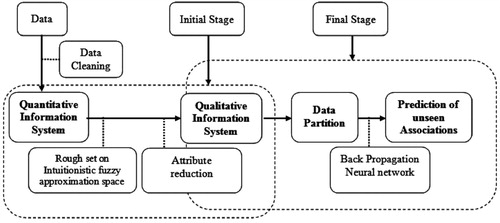
Before we process data at the initial stage, a sequence of cleaning task such as abstracting noise, consistency check and data plenary are carried out to ascertain that the data are as precise as possible. The target data are processed using intuitionistic fuzzy tolerance relation to obtain almost indiscernibility of data values for each attributes. The classification generated produces the $(\alpha ,\beta )$-equivalence classes, where $\alpha$ is the degree of belongingness and $\beta$ the degree of non-belongingness, respectively. It is obvious that the degree of belongingness must be high and degree of non-belongingness must be low to get good appropriate classification. On making the belongingness as 1 (100%) and non-belongingness as 0, the model fails to analyse the information system as each classification will contain exactly one object. It is because of the attribute values present in the system are non-qualitative. The membership and non-membership relation have been premeditated such that the sum of their values lies between [0, 1] and additionally, these functions must be symmetric.

The empirical study that we consider is related to crop suitability prediction of Vellore district of Tamil Nadu. The information system contains attributes such as soil pH, moisture, organic matter etc. It provides information about various agriculture contingency factors of different places along with the crops that are cultivated in these places. A place may not be rich in all agriculture contingency factors for the production of any type of crops. However, out of these, some agriculture contingency factors may have greater importance for the production of a particular crop than the others. On varying the values of $\alpha$ and $\beta$, the factors may deviate from each other. Indeed, if we decrement the value of $\alpha$ and increment the value of $\beta$, progressively the number of factors shall become indispensable. The membership and non-membership relation have been premeditated such that the sum of their values lies between [0, 1] and additionally, these relations must be symmetric. The first requirement necessitates a major of 2 in the denominators of the non-membership functions [6,20].

The degree of belongingness $(\mu )$ and the degree of non-belongingness $(\nu )$ between two objects $x_i$ and $x_j$ is defined in Equations (5) and (6), respectively, where $V_{a_i}^{x_i}$ is the value of the object $x_i$ for the attribute $a_i$ (5) $\begin{array}{rl}{\mu }_R(x_i,x_j)& =1-\frac{|V_{a_i}^{x_i}-V_{a_i}^{x_j}|}{\text{Max}(V_{a_i})}\end{array}$(5) (6) $\begin{array}{rl}{\nu }_R(x_i,x_j)& =1-\frac{|V_{a_i}^{x_i}-V_{a_i}^{x_j}|}{2\times \text{Max}(V_{a_i})}\end{array}$(6) The reduced qualitative information system is divided into training data set of 55% and testing data set of 45%. The training data set is alimented into neural network to predict the decision for the new unseen objects. The testing data are used to validate the training phase and to ensure higher accuracy. The article uses back propagation neural network in the final stage to obtain the decisions. The process consists of three layer such as input layer, hidden layer and output layer, as shown in Figure 2. The attribute values, $a_i;1\le i\le m$ of the training data set are fed in the input layer. In the subsequent hidden layer, the actual mapping between the input and output layer is carried out. The number of hidden nodes is generally computed based on trial and error bases based on mean square error and mean percentile error. Let us assume total number of hidden nodes as h. Let us denote hidden node as $z_j;1\le j\le h$. The output nodes are denoted as $d_k;1\le k\le n$, where $n$ is the total number of objects in the training data set.

Figure 2. Design of back propagation neural network.

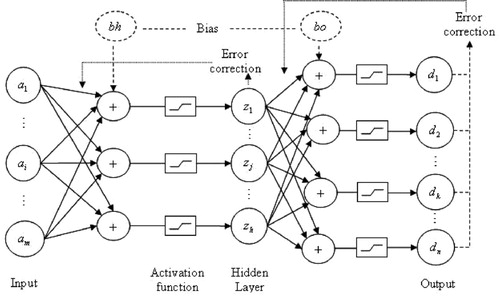
The feed-forward back propagation algorithm [21] is basically gradient descent model where the local minima are identified to converge the input, to the output functions. To facilitate this mean square error between the desired, and actual output is calculated to be minimum. This learning consists of two computational phases such as forward pass and backward pass. Forward pass is a feed-forward propagation of the inputs through the network. The following notions are used in the back propagation algorithm.

1. $A=\left\{a_1,a_2,a_3,\cdots ,a_i,\cdots a_m\right\}$: input attribute values (Training vector); where $m$= 15;

2. $d=\{d_1,d_2,d_3,\cdots ,d_k,\cdots d_n\}$: observed decisions (Target vector);

3. $T=\left\{t_1,t_2,t_3,\cdots ,t_m\right\}$: actual decisions;

4. $z_j$: hidden node where ;

5. $v$: random weight vector connecting the input and hidden layer;

6. $w$: random weight vector connecting the hidden and output layer;

7. $\text{b}{\text{h}}_j$: bias on hidden unit,

8. bo_k: bias on output unit

9. $\text{er}{\text{r}}_k$: error at output node

10. $\text{er}{\text{r}}_j$: error at hidden node $z_j$;

11. $\mathrm{\Delta }v$: weight correction term at the input layer ; $[\mathrm{\Delta }{v}_{ij}{]}_{m\times h}$; $1\le i\le m$;

12. $\mathrm{\Delta }w$: weight correction term at the hidden layer ; $[\mathrm{\Delta }{w}_{jk}{]}_{h\times n};$

13. $\text{LR}$: learning rate;

14. $E_{max}$: maximum number of epochs required for training;

15. epoch: one training loop on considering all the input vector

Algorithm 1(Back Propagation Algorithm)

1. Input: Training Vector ‘$A$’, bias on hidden unit ‘bh’, learning rate ‘LR’

2. Output: The trained data set.

3. Initialise weight vector of the input layer $v=[v_{ij}{]}_{m\times h}$ by small random values, typically between −1 and 1; i.e. $-1\le v_{ij}\le 1$.

4. Initialise weight vector of the hidden layer $w=[w_{jk}{]}_{h\times n}$ by small random values, not necessarily between −1 and 1.

5. Initialise mean square error, MSE = 0; epoch = 0 and learning rate LR.

6. Each input unit receives the input value $a_i$ and transmits this value to all units in the hidden layer.

7. Each hidden unit $z_j$; $1\le j\le h$, compute its interconnection weight $z_{\text{i}{\text{n}}_j}$ as defined below: $z_{\text{i}{\text{n}}_j}=\text{b}{\text{h}}_j+\sum _{i=1}^m(a_i\times v_{ij})$

8. Apply activation function to all the interconnection weight $z_{i{n}_j}$, i.e. $z_j=g(z_{i{n}_j})$ and transmits these values to all the units in the output layer.

9. Each output unit $d_k;k=1,2,\cdots \cdots ,n$ compute its interconnection weight $d_{i{n}_k}$as defined below $d_{\text{i}{\text{n}}_k}=\text{b}{\text{o}}_h+\sum _{j=1}^h{z}_j\times w_{jk}$

10. Apply activation function to all the interconnection weight $d_{i{n}_k}$; $d_k=g(d_{i{n}_k})$.

11. For each output unit $d_k;k=1,2,\cdots \cdots ,n$, compute the mean square error MSE, and average mean square error (AMSE), is given $\text{MSE}=\text{MSE}+(t_k-d_k{)}^2;\text{ASME}=\frac{\text{MSE}}{n}$

12. Increase epoch by 1, i.e. epoch = epoch + 1

13. If (AMSE ≤ 0.5) or (epoch =$E_{max}$), then stop training; else repeat steps 9–12.

14. Each output unit $d_k;k=1,2,\cdots \cdots ,n$ receives a target pattern corresponding to an input pattern. Compute the error term as given below ${\delta }_k=d_k(1-d_k)(t_k-d_k)$

15. Each hidden unit $z_j;j=1,2,\cdots \cdots ,h$ compute its error interconnection weight as defined below ${\delta }_{\text{i}{\text{n}}_j}=\sum _{k=1}^n{\delta }_k{w}_{jk}$

16. The error information term can be calculated as ${\delta }_j={\delta }_{\text{i}{\text{n}}_j}{z}_j(1-z_j)$

17. Each output unit $d_k;k=1,2,\cdots \cdots ,n$ updates its weights by using weight connection term $\mathrm{\Delta }{w}_{jk}$as $\mathrm{\Delta }{w}_{jk}=\text{LR}\ast {\delta }_k{z}_j\text{ for }j=1,2,\cdots ,h$

18. The bias correction term $\mathrm{\Delta }\text{b}{\text{o}}_k$, given as $\mathrm{\Delta }\text{b}{\text{o}}_k=\alpha {\delta }_k$. Thus, we have $w_{jk}(new)=w_{jk}(old)+\mathrm{\Delta }{w}_{jk}$ and $b{o}_k(\text{new})=b{o}_k(\text{old})+\mathrm{\Delta }b{o}_k$

19. Each hidden unit $z_j;j=1,2,\cdots \cdots ,h$ updates its weights by using weight correction term $\mathrm{\Delta }{v}_{ij}$ as below $\mathrm{\Delta }{v}_{ij}=\text{LR}\ast {\delta }_j{a}_i\text{ for }i=1,2,\cdots ,m$

20. The bias correction term $\mathrm{\Delta }\text{b}{\text{h}}_j$, given as $\mathrm{\Delta }\text{b}{\text{h}}_j=\alpha {\delta }_j$. Thus, we have the following equations and then go to step 4 and repeat the process. $v_{ij}(\text{new})=v_{ij}(\text{old})+\mathrm{\Delta }{v}_{ij}$ and $\text{b}{\text{h}}_j(\text{new})=\text{b}{\text{h}}_j(\text{old})+\mathrm{\Delta }\text{b}{\text{h}}_j$

5. An Empirical Study on Crop Suitability Prediction

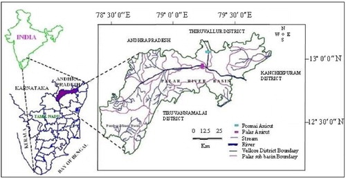
The major objective of the research model taken in to consideration is to analyse and to predict the suitable place for cultivating the agriculture crop to yield maximum benefit with the existing resources on a various period of time. Usually, a layman depends on some agriculture research centre or some advice from the agriculture officers to lay the crops on their land. But in practical, it is time-consuming process. The proposed model act as a tool for a layman to identify the crop to be cultivated in a place based on the richness of various components of the specific crop. To make apparent research model, we considered a real-life problem pertaining to crop cultivation in Vellore district of Tamil Nadu. Historical data from 2011 to 2014 of Krishi Vigyan Kendra of Vellore district are collected. The major resource such as soil and land classification is considered based on the survey of agriculture department of Vellore district, Tamil Nadu. Additionally, Tamil Nadu state agriculture departments has divided Tamil Nadu into seven agro-climate zones such as cauvery delta zone, north-eastern zone, western zone, north western zone, high altitude zone, southern zone and high rainfall zone based on various components such as rainfall, soil, irrigation, another physical and ecological features. Among this, Vellore district is categorised under north-eastern zone which entertains an average rainfall of 1099.1 mm per year. The index map as per Krishi Vigyan Kendra of the study area is depicted in Figure 3.

Figure 3 Index map of the study area.

Furthermore, Vellore district has been distributed into nine agricultural divisions in 2011 and is further separated into 20 blocks. A total of 4799 villages of 20 blocks were documented according to Krishi Vigyan Kendra whose main occupation is agriculture. Most of the villages produce major agricultural crops such as paddy, cholam, cumbu, ragi, samai, red gram, black gram etc. Apart from this, some villages produce horticulture crops such as banana, mango, guava, sapota etc. as fruit crops and also vegetable crops such as brinjal, tomato, onion, sweet potato etc. Some also yield flower crops and spices such as jasmine, chrysanthemum, marigold and chillies, turmeric, respectively. In this paper, effort has been taken to collect data from some villages whose main occupation is agriculture. The administrative block boundary map of Vellore district in 2009 on which the study is carried out is shown in Figure 4. For better understanding, the agriculture divisions along with the blocks are presented in Table 2.

Figure 4. Administrative blocks of the study area.

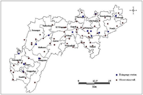
Table 2. Agricultural divisions in Vellore district

S. no.	Agriculture division	Blocks
1.	Vellore (1)	Vellore, Kaniyambadi, Anaicut
2.	Gudiyatham (2)	Gudiyatham, K.V.Kuppam and Katpadi
3.	Vaniyambadi (3)	Alangayam, Madhanur and Pernambattu
4.	Tirupathur (4)	Tirupathur, Kandhili, Natrampalli and Jolarpet
5.	Walajah (5)	Walajah and Sholingur
6.	Arcot (6)	Arcot and Thimiri
7.	Arakonam (7)	Arakonam, Nemili, Kaveripakkam
8	Ambur (8)	Madhanur
9	Katpadi (9)	K.V. Kuppam, and Katpadi

The most common attributes for crop production of Vellore district includes, soil component, water components, rainfall during north-east monsoon, rainfall during south-west monsoon, organic manure, moisture etc. Soil and water components are different at various places and depend on several factors. So, it is essential to identify the availability of NPK (Nitrogen, Phosphorus, Potassium) ratio on soil at congruous stage afore cultivation. It minimises the use of inorganic chemical fertilisers. These parameters form the attribute set of analysis. The data collected from Krishi Vigyan Kendra and agriculture department are consolidated and presented in Tables 3 and 4. Table 3 represents the notations of various attributes, possible values and max range value of each attribute whereas Table 4 depicts the consolidated sample data considered to our study.

Table 3. Notation representation table

Attributes	Abbreviation	Notation	Possible values	Max value
Soil pH	SPH	$a_1$	[5.4–8.5]	8.5
Moisture	MOI	$a_2$	[5–12.2]	12.2
Organic matter	OM	$a_3$	[0.65–1.98]	1.98
Nitrogen	N	$a_4$	[ 200–800]	800
Phosphorous	P	$a_5$	[ 40–533]	533
Potassium	K	$a_6$	[115–1045]	1045
Copper	Cu	$a_7$	[0.05–2]	2
Zinc	Zn	$a_8$	[ 0.01–2]	2
Manganese	Mn	$a_9$	[0.7–4.6]	4.6
Iron	Fe	$a_{10}$	[1.98–99.6]	99.6
Water pH	WPH	$a_{11}$	[6.2–8.5]	8.5
Calcium	Ca	$a_{12}$	[11–420]	420
Nitrate	NO3	$a_{13}$	[ 16–140]	140
Magnesium rain	Mg	$a_{14}$	[ 21–280]	280
Rainfall R	R	$a_{15}$	[ 773.4–1111.2]	1111.2
Places	PL	$d$	–

Table 4. Sample agriculture information system

Obj.	$a_1$	$a_2$	$a_3$	$a_4$	$a_5$	$a_6$	$a_7$	$a_8$	$a_9$	$a_{10}$	$a_{11}$	$a_{12}$	$a_{13}$	$a_{14}$	$a_{15}$	Places
$x_1$	7.3	9	0.96	350	200	160	1.2	1.8	3.2	61.2	7.3	20	16	226.14	787.9	3
$x_2$	7.2	11.7	0.99	450	130	115	1.2	1.09	1.088	75	8.5	21	17	25	1045.4	1
$x_3$	7.21	11.5	0.91	360	200	645	0.5	1.5	0.8	69	7.1	72.3	45	77.3	1111.2	7
$x_4$	7.35	9.5	0.78	432	40	150	1.6	3.3	1.7	61	7.36	23	63	280	1052.2	6
$x_5$	7.5	7	0.78	200	44	162.86	0.05	1.2	2.49	57	6.3	39	78	259	995	2
$x_6$	5.4	6.1	1.23	560	476	486	0.5	3.5	4.6	47	6.2	40.8	84	166	890	4
$x_7$	7.47	8	1.32	475	120	310	0.45	1.1	1.2	1.98	7.43	11	78	26	999.3	2
$x_8$	6.2	6.7	0.98	345	527	1045	0.9	4.7	2.7	2.2	6.35	80	56	250	894.3	4
$x_9$	6.3	7	1.2	401	222	672	0.05	0.01	0.7	8.4	6.35	53.8	45	21	1037.5	1
$x_{10}$	7.1	5	1.32	400	160	160	1.9	2.1	2.4	51.1	8.3	148	25	176.63	1004.4	2
$x_{11}$	7.45	8	1.67	540	242	370	1.5	5	3.3	8.8	7.41	420	56	110	998.7	7
$x_{12}$	7.2	11.9	1.53	200	160	220	1.8	1.2	3.4	61.4	7.4	20	140	211.55	773.4	3
$x_{13}$	8.5	10	1.52	800	190	340	1.2	2.4	1.8	45	8.31	70	130	120	999	4
$x_{14}$	7.32	12.1	1.98	645	140	120	1.4	2.2	3.5	64	7.42	12	18	27	1008.6	7
$x_{15}$	7.4	9	1.32	450	160	325	1.6	1.6	1.8	62.1	7.2	45	41	23	885.2	3
$x_{16}$	8.47	8	0.65	340	533	477	0.51	2.5	1.68	7.57	7	138	45	71	891.2	5
$x_{17}$	7.1	11.8	0.98	340	349	476	0.5	3.6	0.8	4.5	7.2	128	23	211	1012.6	6
$x_{18}$	5.5	10	0.88	650	170	150	1.1	1.9	4.6	51.5	7.28	60	126	130	880.5	4
$x_{19}$	7.2	8	0.92	460	120	140	1.1	1.2	3.2	60.2	8.11	118	24	69.5	1032.2	1
$x_{20}$	7.21	12.2	1.68	340	480	240	2	3.8	4.2	99.6	7.21	51	57	206.4	1008.1	5

The information system presented in Table 4 provides the information about 20 crops that are cultivated at various blocks of agriculture divisions of Vellore district. The information system contains essential attributes such as soil pH, moisture, organic matter etc. whereas objects are considered as crops. The decision attribute is considered as agricultural division where the particular crop is essentially cultivated to get maximum yield. The main objective of this study is to help farmers in identifying the crops suitable for their land. But the maximum yield rate depends on the various components like soil, water, rainfall etc. But, land and water are the crucial resource in nature. Additionally, a cultivation land may not rich in all the parameters to engender highest productivity. But, these factors are almost indiscernible and hence can be classified by using intuitionistic fuzzy proximity relation.

5.1. Initial Stage of an Empirical Study

This section demonstrates the proposed model by considering data collected from Krishi Vigyan Kendra for extracting information. The collected data contains 26 attributes, out of which to maintain consistency, the core and the reduct is applied for attribute reduction. Thus, the reduced data set is processed with intuitionistic fuzzy proximity relation. To provide a clear understanding, we considered the sample data set presented in Table 4 and employed intuitionistic fuzzy proximity relation. Simultaneously, rough set helps to eliminate the parameters that are superfluous in an information system. The computations are carried out by using Eqnuations (5) and (6) [22]. The results are presented in Table 5 for attribute $a_1$ (Soil pH) and Table 6 for the attribute $a_2$ (Moisture), on considering the random selection of 55% of the total objects (11 objects) shown in Table 4. The process is repeated for all the 15 attributes present in the considered information system. Let $\text{I}{\text{R}}^{a_i},i=1,2,3,\cdots ,15$ be the intuitionistic fuzzy proximity relation corresponding to the attributes $a_i,i=1,2,3,\cdots ,15$. On taking into account the length of the paper, the computation of intuitionistic fuzzy proximity relation for the other attributes is omitted.

Table 5. Intuitionistic fuzzy tolerance relation for the attribute a₁

${\text{IR}}_{(\alpha ,\beta )}^{a_1}$	$x_1$	$x_2$	$x_3$	$x_4$	$x_5$	$x_6^{}$	$x_7$	$x_8$	$x_9$	$x_{10}$	$x_{11}$
$x_1$	1, 0	0.99, 0.01	0.99, 0.00	0.99, 0,00	0.98, 0.01	0.79, 0.11	0.98, 0.01	0.88, 0.06	0.89, 0.06	0.98, 0.01	0.98, 0.01
$x_2$	0.99, 0.01	1,0	1.00, 0.00	0.98, 0.01	0.97, 0.02	0.80, 0.10	0.97, 0.02	0.89, 0.06	0.90, 0.05	0.99, 0.01	0.97, 0.01
$x_3$	0.99, 0.00	1.00, 0.00	1, 0	0.98, 0.01	0.97, 0.02	0.80, 0.10	0.97, 0.01	0.89 0.06	0.90, 0.05	0.99, 0.01	0.97. 0.01
$x_4$	0.99, 0.00	0.98, 0.01	0.98, 0.01	1, 0	0.98, 0.01	0.78, 0.11	0.99, 0.01	0.87, 0.06	0.88, 0.06	0.97, 0.01	0.99, 0.01
$x_5$	0.98. 0.01	0.97, 0.02	0.97, 0.02	0.98, 0.01	1, 0	0.77, 0.12	1.00, 0.00	0.86, 0.07	0.87, 0.07	0.96, 0.02	0.99, 0.00
$x_6$ $x_6$	0.79, 0.11	0.80, 0.10	0.80, 0.10	0.78, 0.11	0.77, 0.12	1,0	0.77,0.12	0.91,0.04	0.90,0.05	0.81,0.09	0.77,0.10
$x_7$	0.98,0.01	0.97,0.02	0.97,0.01	0.99,0.01	1.00,0.00	0.77,0.12	1,0	0.86,0.07	0.87,0.07	0.96,0.02	1.00,0.00
$x_8$	0.88,0.06	0.89,0.06	0.89,0.06	0.87,0.06	0.86,0.07	0.91,0.04	0.86,0.07	1,0	0.99,0.01	0.90,0.05	0.86,0.07
$x_9$	0.89,0.06	0.90,0.05	0.90,0.05	0.88,0.06	0.87,0.07	0.90,0.05	0.87,0.07	0.99,0.01	1,0	0.91,0.04	0.87,0.06
$x_{10}$	0.98,0.01	0.99,0.01	0.99,0.01	0.97,0.01	0.96,0.02	0.81,0.09	0.96,0.02	0.90,0.05	0.91,0.04	1, 0	0.96,0.02
$x_{11}$	0.98,0.01	0.97,0.01	0.97,0.01	0.99,0.01	0.99,0.00	0.77,0.11	1.00,0.00	0.86,0.06	0.87,0.06	0.96,0.02	1, 0

Table 6. Intuitionistic fuzzy proximity relation for the attribute a₂

${\text{IR}}_{(\alpha ,\beta )}^{a_2}$	$x_1$	$x_2$	$x_3$	$x_4$	$x_5$	$x_6^{}$	$x_7$	$x_8$	$x_9$	$x_{10}$	$x_{11}$
$x_1$	1, 0	0.78, 0.11	0.80, 0.10	0.96, 0.02	0.84, 0.08	0.76, 0.12	0.92, 0.04	0.81, 0.09	0.84, 0.08	0.67, 0.16	0.92, 0.04
$x_2$	0.78,0.11	1, 0	0.98, 0.01	0.82, 0.09	0.61, 0.19	0.54, 0.23	0.70, 0.15	0.59, 0.20	0.61, 0.19	0.45, 0.27	0.70, 0.15
$x_3$	0.80,0.10	0.98, 0.01	1, 0	0.84, 0.08	0.63, 0.18	0.56, 0.22	0.71, 0.14	0.61, 0.20	0.63, 0.18	0.47, 0.27	0.71 ,0.14
$x_4$	0.96,0.02	0.82,0.09	0.84,0.08	1, 0	0.80, 0,10	0.72,0.14	0.88,0.06	0.77,0.11	0.80,0.10	0.63,0.18	0.88,0.06
$x_5$	0.84,0.08	0.61,0.19	0.63,0.18	0.80,0.10	1, 0	0.93,0.04	0.92,0.04	0.98,0.01	1.00,0.00	0.84,0.08	0.92,0.04
$x_6{x}_6$	0.76,0.12	0.54,0.23	0.56,0.22	0.72,0.14	0.93,0.04	1, 0	0.84,0.08	0.95,0.02	0.93,0.04	0.91,0.05	0.84,0.08
$x_7$	0.92,0.04	0.70,0.15	0.71,0.14	0.88,0.06	0.92,0.01	0.84,0.08	1, 0	0.89,0.05	0.92,0.04	0.75,0.12	1.00,0.00
$x_8$	0.81,0.09	0.59,0.20	0.61,0.20	0.77,0.11	0.98,0.01	0.95,0.27	0.89,0.05	1, 0	0.98,0.01	0.86,0.07	0.89,0.05
$x_9$	0.84,0.08	0.61,0.19	0.63,0.18	0.80,0.10	1.00,0.00	0.93,0.04	0.92,0.04	0.98,0.01	1, 0	0.84,0.08	0.92,0.04
$x_{10}$	0.67,0.16	0.45,0.27	0.47,0.27	0.63,0.18	0.84,0.08	0.91,0.05	0.75,0.12	0.86,0.07	0.84,0.08	1, 0	0.75,0.12
$x_{11}$	0.92,0.04	0.70,0.15	0.71,0.14	0.88,0.06	0.92,0.04	0.84,0.08	1.00,0.00	0.89,0.05	0.92,0.04	0.75,0.12	1, 0

On considering the degree of membership and non-membership values as $\alpha \le 0.95$, $\beta \le 0.3$, it can be seen from Table 5 that $\mu (x_1,x_1)=1.00$, $\nu (x_1,x_1)=0$; $\mu (x_1,x_2)=0.99$, $\nu (x_1,x_2)=0.01$; $\mu (x_2,x_3)=1.00$, $\nu (x_2,x_3)=0$; $\mu (x_3,x_4)=0.98$, $\nu (x_3,x_4)=0.01$; $\mu (x_4,x_5)=0.98$, $\nu (x_4,x_5)=0.01$; $\mu (x_5,x_7)=1.00$, $\nu (x_5,x_7)=0$; $\mu (x_7,x_{10})=0.96$, $\nu (x_7,x_{10})=0.02$; $\mu (x_{10},x_{11})=0.96$, $\nu (x_{10},x_{11})=0.02$; $\mu (x_{11},x_1)=0.98$ and $\nu (x_{11},x_1)=0.01$.

Therefore, the objects $x_1,x{}_2,x_3,x_4,x_5,x_7,x_{10},x_{11}$ are $(\alpha ,\beta )-$indiscernible. Also, the object $x_6$ is not $(\alpha ,\beta )-$indiscernible with any other objects. Thus, the almost equivalence class generated is given as $U/R_{(\alpha ,\beta )}^{a_1}=\{\{x_1,x_2,x_3,x_4,x_5,x_7,x_{10},x_{11}\},\{x_6\},\{x_8,x_9\}\}$ In the same way, the computation is conceded for 20 crops (objects) and the almost equivalence class obtained for the attributes $a_i,i=1,2,3\dots 15$ are given below. It is seen that the attribute values of soil pH $(a_1)$ are classified into four categories, namely very high, high, moderate and low. Alike, the attribute values of other attributes are also classified. $\begin{array}{rl}& U/{\text{IR}}_{(\alpha ,\beta )}^{a_1}\\ & =\{\{x_1,x_2,x_3,x_4,x_5,x_7,x_{10},x_{11},x_{12},x_{14},x_{15},x_{17},x_{19},x_{20}\},\{x_8,x_9\},\{x_{13},x_{16}\},\{x_6,x_{18}\}\}\end{array}$ $\begin{array}{rl}U/{\text{IR}}_{(\alpha ,\beta )}^{a_2}& =\{\{x_1,x_4,x_{13},x_{15},x_{18}\},\{x_5,x_6,x_8,x_9\},\{x_2,x_3,x_{12},x_{14},x_{17},x_{20}\},\{x_7,x_{11},x_{16},x_{19}\},\\ & \{x_{10}\}\}\end{array}$ $\begin{array}{rl}U/{\text{IR}}_{(\alpha ,\beta )}^{a_3}& =\{\{x_1,x_2,x_3,x_4,x_5,x_8,x_{17},x_{18},x_{19}\},\{x_6,x_7,x_9,x_{10},x_{15}\},\{x_{11},x_{20}\},\{x_{12},x_{13}\},\\ & \{x_{14}\},\{x_{16}\}\}\end{array}$ $\begin{array}{rl}U/{\text{IR}}_{(\alpha ,\beta )}^{a_4}& =\{\{x_1,x_2,x_3,x_4,x_7,x_8,x_9,x_{10},x_{15},x_{16},x_{17},x_{19},x_{20}\},\{x_5,x_{12}\},\{x_{14},x_{18}\},\{x_6,x_{11}\},\\ & \{x_{13}\}\}\end{array}$ $\begin{array}{rl}U/{\text{IR}}_{(\alpha ,\beta )}^{a_5}& =\{\{x_1,x_2,x_3,x_7,x_9,x_{10},x_{11},x_{12},x_{13},x_{14},x_{15},x_{17},x_{18},x_{19}\},\{x_6,x_{20}\},\{x_8,x_{16}\},\\ & \{x_4,x_5\}\}\end{array}$ $\begin{array}{rl}U/{\text{IR}}_{(\alpha ,\beta )}^{a_6}& =\{\{x_1,x_2,x_4,x_5,x_{10},x_{12},x_{14},x_{18},x_{19},x_{20}\},\{x_6,x_{16},x_{17}\},\{x_3,x_9\},\{x_7,x_{11},x_{13},\\ & x_{15}\}\}\end{array}$ $\begin{array}{rl}U/{\text{IR}}_{(\alpha ,\beta )}^{a_7}& =\{\{x_1,x_2,x_{13},x_{18},x_{19}\},\{x_3,x_6,x_7,x_{16},x_{17}\},\{x_4,x_5,x_9,x_{11},x_{14},x_{15}\},\{x_{10},x_{12},\\ & x_{20}\},\{x_8\}\}\end{array}$ $\begin{array}{rl}U/{\text{IR}}_{(\alpha ,\beta )}^{a_8}& =\{\{x_1,x_3,x_{10},x_{13},x_{14},x_{15},x_{16},x_{18}\},\{x_4,x_6,x_{17},x_{20}\},\{x_2,x_5,x_7,x_{12},x_{19}\},\{x_9\},\\ & \{x_{11}\},\{x_8\}\}\end{array}$ $\begin{array}{rl}U/{\text{IR}}_{(\alpha ,\beta )}^{a_9}& =\{\{x_1,x_{11},x_{12},x_{14},x_{19}\},\{x_2,x_7\},\{x_3,x_9,x_{17}\},\{x_4,x_{13},x_{15},x_{16}\},\{x_5,x_8,x_{10}\},\{x_6,\\ & x_{18}\},\{x_{20}\}\}\end{array}$ $\begin{array}{rl}U/{\text{IR}}_{(\alpha ,\beta )}^{a_{10}}& =\{\{x_1,x_3,x_4,x_5,x_{12},x_{14},x_{15},x_{19}\},\{x_2\},\{x_6,x_{10},x_{13},x_{18}\},\{x_7,x_8,x_9,x_{11},x_{17},\\ & x_{16}\},\{x_{20}\}\}\end{array}$ $\begin{array}{rl}U/{\text{IR}}_{(\alpha ,\beta )}^{a_{11}}& =\{\{x_1,x_3,x_4,x_7,x_{11},x_{12},x_{14},x_{15},x_{16},x_{17},x_{18},x_{20}\},\{x_2,x_{10},x_{13},x_{19}\},\{x_5,x_6,x_8,\\ & x_9\}\}\end{array}$ $\begin{array}{rl}U/{\text{IR}}_{(\alpha ,\beta )}^{a_{12}}& =\{\{x_1,x_2,x_4,x_5,x_6,x_7,x_{12},x_{14},x_{15}\},\{x_3,x_8,x_9,x_{13},x_{18},x_{20}\},\{x_{10},x_{16},x_{17},x_{19}\},\\ & \{x_{20}\},\{x_{11}\}\}\end{array}$ $\begin{array}{rl}U/{\text{IR}}_{(\alpha ,\beta )}^{a_{13}}& =\{\{x_1,x_2,x_{10},x_{14},x_{17},x_{19}\},\{x_3,x_9,x_{15},x_{16}\},\{x_4,x_8,x_{11},x_{20}\},\{x_5,x_6,x_7\},\{x_{12},\\ & x_{13},x_{18}\}\}\end{array}$ $\begin{array}{rl}U/{\text{IR}}_{(\alpha ,\beta )}^{a_{14}}& =\{\{x_1,x_{12},x_{17},x_{20}\},\{x_2,x_7,x_9,x_{14},x_{15}\},\{x_3,x_{16},x_{19}\},\{x_4\},\{x_5,x_8\},\{x_6,x_{10}\},\\ & \{x_{11},x_{13},x_{18}\}\}\end{array}$ $\begin{array}{rl}U/{\text{IR}}_{(\alpha ,\beta )}^{a_{15}}& =\{\{x_1,x_{12}\},\{x_2,x_3,x_4,x_5,x_7,x_9,x_{10},x_{11},x_{13},x_{14},x_{17},x_{19},x_{20}\},\{x_6,x_8,x_{16},x_{15},\\ & x_{18}\}\}\end{array}$ Unlike the attribute $a_1$, the attribute $a_2$ is categorised into five categories, namely very high, high, moderate, low and very low. Similarly, the attributes $a_3,a_4,a_5,a_6,a_7,a_8,a_9,a_{10},$ $a_{11},a_{12},a_{13},a_{14},a_{15}$ are categorised into 6, 5, 4, 5, 5, 6, 7, 6, 3, 4, 6, 7 and 3 categories, respectively. The maximum number of categories is observed to be 7. Let the categories are very high (Vh), high (H), moderate (M), low (L), very low (Vl), poor (P) and negligible (Ne). This condenses the quantitative information system into qualitative information system, as shown in Table 7.

5.2. Final Stage of Empirical Study

The steps involved in the final process of the empirical study are discussed in this section. Predicting the places for cultivating agricultural crops on real data sets is considered as the main objective of this article. We used back propagation feed-forward neural network (BPNN) method for the investigation taken into consideration. The method is based on minimising the mean square error (MSE) and mean percentile error (MPE). The back propagation algorithm as discussed in Section 5.4 is used to train the data set. Based on the input attribute values, $y_{\text{in}}$ and $y_{\text{out}}$ are computed as discussed in Equations (3) and (4), respectively.

Table 7. Qualitative information system of sample dataset

Obj.	$a_1$	$a_2$	$a_3$	$a_4$	$a_5$	$a_6$	$a_7$	$a_8$	$a_9$	$a_{10}$	$a_{11}$	$a_{12}$	$a_{13}$	$a_{14}$	$a_{15}$	Places
$x_1$	H	H	Vl	L	M	Vl	M	L	M	M	M	Vl	P	M	L	Alangayam
$x_2$	H	Vh	Vl	L	M	Vl	M	Vl	Vl	H	H	Vl	P	Ne	H	Anaicut
$x_3$	H	Vh	Vl	L	M	H	Vl	L	Ne	M	M	L	Vl	P	H	Arakonam
$x_4$	H	H	Vl	L	L	Vl	H	M	P	M	M	Vl	L	Vh	H	Arcot
$x_5$	H	L	Vl	Vl	L	Vl	H	Vl	L	M	L	Vl	M	H	H	Gudiyatham
$x_6$	L	L	L	M	H	M	Vl	M	Vh	L	L	Vl	M	L	M	Jolarpet
$x_7$	H	M	L	L	M	L	Vl	Vl	Vl	Vl	M	Vl	M	Ne	H	K V Kuppam
$x_8$	M	L	Vl	L	Vh	Vh	L	H	L	Vl	L	L	L	H	M	Kandeli
$x_9$	M	L	L	L	M	H	H	P	Ne	Vl	L	L	Vl	Ne	H	Kaniyambadi
$x_{10}$	H	Vl	L	L	M	Vl	Vh	L	L	L	H	H	P	L	H	Katpadi
$x_{11}$	H	M	H	M	M	L	H	Vh	M	M	M	Vh	L	Vl	H	Kaveripakkam
$x_{12}$	H	Vh	M	Vl	M	Vl	Vh	Vl	M	M	M	Vl	Vh	M	L	Madhanur
$x_{13}$	Vh	H	M	Vh	M	L	M	L	P	L	H	L	H	Vl	H	Natrampalli
$x_{14}$	H	Vh	Vh	H	M	Vl	H	L	M	M	M	Vl	P	Ne	H	Nemili
$x_{15}$	H	H	L	L	M	L	H	L	P	M	M	Vl	Vl	Ne	M	Pemambattu
$x_{16}$	Vh	M	P	L	Vh	M	Vl	L	P	Vl	M	H	Vl	P	M	Sholingur
$x_{17}$	H	Vh	Vl	L	M	M	Vl	M	Ne	Vl	M	H	P	M	H	Thimiri
$x_{18}$	L	H	Vl	H	M	Vl	M	L	Vh	L	M	L	H	Vl	M	Tirupathur
$x_{19}$	H	M	Vl	L	M	Vl	M	Vl	M	M	H	H	P	P	H	Vellore
$x_{20}$	H	Vh	H	L	H	Vl	Vh	M	H	Vh	M	L	L	M	H	Walajahpet

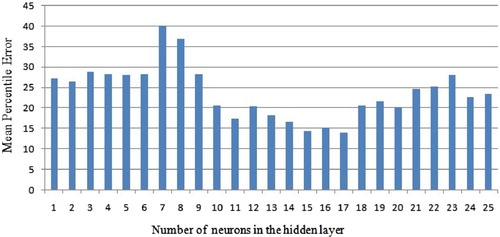
Back propagation neural network is a supervised learning technique and so the training process can be terminated by declaring certain conditions. The process terminates if the network has procured the average mean square error (MSE) ≤0.5 or the number of pre-defined epochs. Generally, the number of neurons in the hidden layer is identified through trial and error basis based on MSE and MPE to get better performance. The weight coefficient is recorded, so as to identify the effect of the number of hidden neurons acquired to map the input space and the output space. The result of recording shows that the best result is obtained at 17th hidden neurons in a single hidden layer architecture. While preserving the number of neurons as 17 and the learning rate as 0.5, the MSE obtained as 0.188 with the number of epochs as 300. It is also observed that on increasing the number of hidden neurons as much as more than 200 and the number of hidden layers ≥2, the combinations could not achieve the MSE ≤0.188. So, the analysis is restricted to 17 hidden neurons with a single hidden layer. The results of MSE and MPE against the number of neurons are depicted in Figures 5 and 6, respectively.

Figure 5. Number of hidden nodes using MSE.

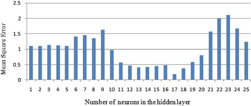
Figure 6. Number of hidden nodes using MPE.

The training model is then tested with rest nine objects $x_{12},x_{13},x_{14},x_{15},x_{16},x_{17},x_{18},x_{19},x_{20}$ of qualitative information system presented in Table 7. The validation process is presented in Table 8. From Table 8, it is clear that all objects are correctly classified. Thus, the accuracy of the training process is computed as below $\text{Accuracy = }\frac{\text{Supporting}\text{objects}}{\text{Total}\text{number}\text{of}\text{objects}}\text{ = }\frac{9}{9}=100\mathrm{\%}$ But, in the experimental study, it is observed that the average classification accuracy of 93.7% is achieved on increasing the number of objects to 2193. The validation process along with an experimental comparative study was carried out in Section 6 to check its viability.

Table 8. Validating the training data

Obj.	$a_1$	$a_2$	$a_3$	$a_4$	$a_5$	$a_6$	$a_7$	$a_8$	$a_9$	$a_{10}$	$a_{11}$	$a_{12}$	$a_{13}$	$a_{14}$	$a_{15}$	Recorded places	Observed Places
$x_{12}$	H	Vh	M	Vl	M	Vl	Vh	Vl	M	M	M	Vl	Vh	M	L	8	8
$x_{13}$	Vh	H	M	Vh	M	L	M	L	P	L	H	L	H	Vl	H	4	4
$x_{14}$	H	Vh	Vh	H	M	Vl	H	L	M	M	M	Vl	P	Ne	H	7	7
$x_{15}$	H	H	L	L	M	L	H	L	P	M	M	Vl	Vl	Ne	M	3	3
$x_{16}$	Vh	M	P	L	Vh	M	Vl	L	P	Vl	M	H	Vl	P	M	5	5
$x_{17}$	H	Vh	Vl	L	M	M	Vl	M	Ne	Vl	M	H	P	M	H	6	6
$x_{18}$	L	H	Vl	H	M	Vl	M	L	Vh	L	M	L	H	Vl	M	4	4
$x_{19}$	H	M	Vl	L	M	Vl	M	Vl	M	M	H	H	P	P	H	1	1
$x_{20}$	H	Vh	H	L	H	Vl	Vh	M	H	Vh	M	L	L	M	H	5	5

6. Comparative Analysis and Results

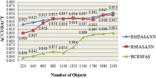
Experimental analysis has been carried out to get the efficiency of the proposed model, RSIFASANN. The experiments were conducted with a computer having Intel Pentium Processor, 8GB RAM, Windows 10 operating system and MATLAB R2008a. For analysis purpose, data are collected from Krishi Vigyan Kendra (KVK), Vellore, India. The data for 4799 villages were collected. But after careful observation, it is identified that 2193 villages are having agriculture crop production as their main occupation. The intuitionistic fuzzy proximity relation is employed on whole data for getting almost equivalence classes. This phase changes the quantitative information system to qualitative information system. Further, the qualitative data set of 2193 objects are validated with the training model. Additionally, we have chosen a model which integrates Bayesian classification and RSFAS (BCRSFAS) [12]. Also, the proposed model is compared with the previous work of hybridising RSFAS with Neural network as (RSFASANN). We have randomly selected 220 objects and predicted the decision using BCRSFAS and the proposed model RSIFASANN. Further, the number of objects is randomly increased by 220. The classification accuracy against both the models was checked. The process is repeated till the whole data set of 2193 objects. The results obtained are presented in Table 9. The average accuracy obtained by the proposed model RSIFASANN is 93.7. The accuracy of model RSIFASANN is higher than the accuracy of RSFASANN and the accuracy of RSFASANN is higher than BCRSFAS.

Table 9. Comparative analysis and results.

	Supporting objects			Accuracy obtained
Objects	RSIFASANN	RSFASANN	BCRSFAS	RSIFASANN	RSFASANN	BCRSFAS
220	203	198	184	0.923	0.900	0.836
440	408	399	370	0.927	0.907	0.841
660	616	611	560	0.933	0.926	0.848
880	823	825	750	0.935	0.938	0.852
1100	1031	1030	935	0.937	0.936	0.850
1320	1236	1240	1140	0.936	0.939	0.864
1540	1443	1443	1369	0.937	0.937	0.889
1760	1656	1645	1578	0.941	0.935	0.897
1980	1875	1874	1779	0.947	0.946	0.898
2193	2090	2076	1975	0.953	0.947	0.901
Average accuracy =				0.937	0.931	0.868

The comparative graph is depicted in Figure 7 for better visualisation. From the above analysis, it is clear that the classification accuracy of RSIFASANN is higher than the other two models and hence can be considered as a better model.

Figure 7. Experimental comparative graph.

6.1. N-fold Cross-validation

Generally, a classifier is induced from the training data using a learning algorithm. It is a known fact that every classifier is associated with some prediction error. But, the prediction error is unknown, and it is difficult to calculate. At the same time, it is essential to estimate the error from the data while analysing the data in training phase. This error which is estimated based on the data considered is called the estimated predicted error. This estimated predictor error is to be validated by means of its variance and bias.

In the proposed technique, the data set is divided into training (55%) and testing data (45%). Back propagation algorithm is used as the classifier and the estimated predicted error is calculated based on the means square error and mean percentile error, by training the model with varied number of learning rate. The obtained MSE is observed as 0.188 on training the model with one hidden layer. Even though, the model is tested with more than one hidden layer, but the results are convincing enough to have a single hidden layer. Thus, out of 2193 data, the training data of 1203 data set were trained using back propagation algorithm and the testing data of 990 are tested with the least means square error. Further, the validation is performed using N-fold cross-validation and the results are presented as follows.

In N-fold cross-validation, the data set is divided into N-folds, a classifier is learned using (N – 1) folds, and an error value is calculated by testing the classifier in the remaining fold. Finally, the N-CV estimation of the error is the average value of the errors committed in each fold. Thus, the N-CV error estimator depends on two factors: the training set and the partition into folds.

The experimental analysis is performed using R language. The data set contains 15 conditional at tributes and one predictive attribute. The data set is divided with various number of folds such as N = 10, 15, 20 and 25. The MSE are recorded with respect to various fold values. A sample of the results computed using R language for N = 10 is given in Figure 8, and the overall MSE is recorded in Figure 9. The mean square error obtained for fold 1 is 2.6, whereas the overall mean square error obtained is 2.44. We have analysed the mean square error and overall mean square error on varying N and is presented in Table 10.

Figure 8. Mean square error of Fold 1 for N = 10.

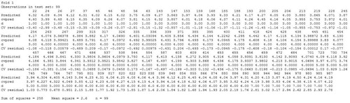
Figure 9. Overall mean square error over all folds for N = 10.

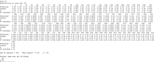
Table 10. Overall mean square error across various folds

Number of folds (N)	Overall MSE	Observations in test set
10	2.44	99
15	2.43	66
20	2.44	49
25	2.44	39
30	2.43	33
Average MSE	0.2436

It is seen from the Table 10 that the average MSE obtained is greater than the average MSE obtained using neural network. Thus, we can say the validation carried out by hybridising rough computing with neural network provides better accuracy in prediction.

7. Conclusion

In this paper, we hybridised RSIFAS with neural network for the prediction of unseen associations of attribute values. The initial process of the proposed model reduces quantitative information system to qualitative information system using RSIFAS. The final process predicts the decision of unseen associations using back propagation neural network. The model is analysed over 20 blocks of Vellore district, Tamil Nadu. The experimental analysis depicts that the proposed model attained the average classification accuracy of 93.7%, whereas that of BCRSFAS is 86.8%. It indicates that the proposed model has 6.9% more classification accuracy than BCRSFAS. Additionally, it facilitates the farmers to take decision on the crops to be cultivated on their land.

Disclosure statement

No potential conflict of interest was reported by the author(s).

Additional information

Notes on contributors

A. Anitha

Dr. A. Anitha is an Associate Professor in the School of Information Technology at VIT, Vellore, India. She received the MCA degree from Adhi Parasakthi College of Science, Kalavai, Tamil Nadu, India. She has published many international journal and conference papers to her credit. Her research interest includes data mining, fuzzy logic, neural network and rough sets. She is associated with the professional bodies CSI.

D. P. Acharjya

Dr. D. P. Acharjya is a Professor in the School of Computing Sciences and Engineering at VIT, Vellore, India. He received his MSc from NIT, Rourkela, India; M. Tech. in Computer Science from Utkal University, India; and PhD in Computer Science from Berhampur University, India. He has been awarded the Gold Medal in M. Sc.; Eminent Academician Award; Outstanding Educator and Scholar Award; The Best Citizens of India Award; and Bharat Vikas Award from various organizations of India. He has authored 84 international and national journal and conference papers. Besides, he has published 4 books and 17 book chapters with international publishers. In addition, he has edited 7 books with international publishers like CRC Press; Springer; and IGI Global, USA. His research interest includes rough sets, knowledge representation, machine learning, bio-inspired computing, and business intelligence. He is associated with many professional bodies, such as ACM, IACSIT, IAENG, CSTA, IRSS, CSI, ISTE, OITS, ISIAM, IMS, and AMTI.

References

- Zadeh LA. Fuzzy sets. Inf Control. 1965;8:338–353.
- Pawlak Z. Rough sets. Int J Comp Inform Sci. 1982;11:341–356.
- Pawlak Z. Rough sets – theoretical aspects of reasoning about data. Dordrecht: Kluwer Academic Publishers; 1991.
- De SK. Some aspects of fuzzy sets, rough sets and intuitionistic fuzzy sets [PhD Thesis]. Kharagpur: IIT, India; 1999.
- Acharjya DP, Tripathy BK. Rough sets on fuzzy approximation spaces and applications to distributed knowledge systems. Int J Artif Intell Soft Comput Inderscience. 2008;1(1):1–14.
- Acharjya DP, Tripathy BK. Rough sets on intuitionistic fuzzy approximation spaces and knowledge representation. Int J Artif Int Comput Res. 2009;1 (1):29–36.
- Molodstov D. Soft set theory-first results. Comp Math Appl. 1999;37(4/5):19–31.
- Peters J. Near sets-general theory about nearness of objects. Appl Math Sci. 2007;1:2609–2629.
- Dubois D, Prade H. Rough fuzzy sets and fuzzy rough set. Int J Gen Syst. 1990;17(2/3):191–209.
- Liu G. Rough set theory based on two universal sets and its applications. Knowl Base Syst. 2010;23:110–115.
- Smarandache F. Neutrosophic set – a generalization of the intuitionistic fuzzy set. Int J Pure Appl Math. 2005;24:287–297.
- Acharjya DP, Roy D, Rahaman AM. Prediction of missing associations using rough computing and Bayesian classification. Int J Intell Syst Appls. 2012;4 (11):1–13.
- Das TK, Acharjya DP. A decision making model using soft set and rough set on fuzzy approximation spaces. Int J Intel Syst Technol Applic . 2014;13(3):170–186.
- Anitha A, Acharjya DP. Neural network and rough set hybrid scheme prediction of missing associations. Int J Bioinform Res Appl. 2015;11(6):503–524.
- Ahn BS, Cho SS, Kim CY. The integrated methodology of rough set theory and artificial neural network for business failure prediction. Expert Syst Appl. 2000;18(2):65–74.
- Rao DVJ, Mitra P. A rough association rule based approach for class prediction with missing attribute values). Proceedings of the 2nd Indian international Conference on Artificial Intelligence; 2005. 20–22.
- Atanasov KT. Intuitionistic fuzzy sets. Fuzzy Sets Syst. 1986;20:87–96.
- Rumelhart DE, McClelland JL. Parallel distributed processing: exploration in microstructure of cognition. Cambridge: Foundations MIT Press; 1986.
- Lippmann RP. An introduction to computing with neural nets. IEEE ASSP Mag. 1987;4(1): 4–22.
- Acharjya DP. Knowledge extraction from information system using rough computing. In: M Usman, editor. Improving knowledge discovery through the integration of data mining techniques. IGI Global, Pennsylvania, USA, 2015, p. 161–182.
- Hecht Nielsen R. Theory of the backpropagation neural network). Proceedings of the international Joint Conference on neural networks, 1 (1989), 593–605.
- Tripathy BK, Acharjya DP. Knowledge mining using ordering rules and rough sets on fuzzy approximation Spaces. Int J Adv Sci Techn. 2010;1(3):41–50.