
 ?Mathematical formulae have been encoded as MathML and are displayed in this HTML version using MathJax in order to improve their display. Uncheck the box to turn MathJax off. This feature requires Javascript. Click on a formula to zoom.
Abstract
Purpose: This research analyses the optimal inventory strategy for a deteriorating product with imprecise deterioration rate in a single supplier-buyer supply chain system with realistic factors.
Design/methodology/approach: The integration of production and distribution inventory system is crucial in practice for minimizing a firm's cost while the effect of deterioration cannot be ignored as it affects the entire inventory system. Nowadays managers have begun to recognize that effectively managing deterioration risks in their business operations plays an important role in successfully managing their inventories. Here, the deterioration rate is treated as the triangular fuzzy number. Also we use the extension principle method to define the membership function of the fuzzy total cost and defuzzify by the centroid to find the estimate of the total cost in the fuzzy sense.
Findings: A methodology has been proposed through mathematical model which involves designing an iterative algorithm to achieve optimal decisions such as order lot-size and total number of deliveries from the supplier to buyer.
Originality value: The effects of varying the central parameter values on the optimal solution are performed by numerical and sensitivity analysis so as to highlight the differences between crisp and the fuzzy cases.
1. Introduction
Deterioration of many items such as chemicals, volatile liquids, medicines, blood banks and some other goods during the storage period is non-negligible in the real-world problem. In general, deterioration is defined as the decay, damage, evaporation, spoilage and obsolescence of stored items and it results in decreasing usefulness [Citation1]. Therefore, it is very important to discuss the deteriorating behaviour of such type of items. Yang and Wee [Citation2] proved that the integrated policy results in an impressive cost reduction when it is compared with the independent decisions made by the vendor and the buyers. Consequently, the integration between supplier and buyer for improving the performance of inventory control has received a great deal of attention and the integrated approach has been examined for years (for instance, [Citation3–9]). Yan et al. [Citation5] developed production-distribution inventory model with the considerations of constant deterioration. Sarkar [Citation6] modified Yan et al.'s [Citation5] model by considering three types of continuous probabilistic deterioration function. Lee and Kim [Citation7] developed an optimal policy for a single-vendor single-buyer integrated production-distribution inventory system with both deteriorating and defective items under the consideration of constant deteriorating rate. Chayanika et al. [Citation8] developed a sustainable supply chain model for a single-manufacturer and a single-buyer's integrated approach by considering item deterioration and imperfect production simultaneously.
Those studies share one common characteristic that the deterioration rate in the models is precisely known. However, in real world applications, the deterioration rate of the items in the model might be in – exact and imprecise in nature. For instance, the deterioration caused by a rise or fall in temperature due to breakdown or accidental damage to the refrigeration equipment or non-operation of the controlling devices of such equipment. These issues are probably uncertain in the real life environment. On the other hand, many potential factors such as properties of products and/or change of environment may affects the rate of deterioration in the practical marketing. There are also situations that the data cannot be collected without errors. Hence we can observe that the rate of deterioration probably has a little disturbance due to various uncertainties. Today the uncertainties are often significant and thus the models need to account for them. Sometimes the uncertainties can be modelled stochastically, but quite often, they cannot be captured with probabilistic means, but only from expert opinions within the companies. This is typically the case with new products, and products with very large seasonal and other unknown variations. For these kinds of uncertainties it is possible to use fuzzy numbers instead of probabilistic approaches.
Fuzzy set theory, introduced by Zadeh [Citation10], has been receiving substantial attention amongst researchers in production and inventory management. Several authors have applied the fuzzy set concepts to deal with the inventory control problems (e.g. see [Citation11–19]). Ishii and Konno [Citation11] fuzzified the shortage cost to an L-fuzzy number in the classical newsboy problem. A backorder inventory model which fuzzifies the order quantity as triangular and trapezoidal fuzzy numbers and keeps the shortage cost as a crisp parameter was developed by Yao and Lee [Citation12]. Then Yao and Chiang [Citation13] developed an EOQ model with the total demand and the unit carrying cost being triangular fuzzy numbers. They used the signed distance and the centroid as defuzzification methods. An inventory model for a deteriorating item with stock dependent demand is developed by Roy et al. [Citation14] under two storage facilities over a random planning horizon. Mishra and Soni [Citation15] developed an economic production models with finite production rate and fuzzy deterioration rate. In a recent article, Liu [Citation16] developed a solution for fuzzy integrated production and marketing planning based on extension principle method.
The main purpose of this research is to present an extensive integrated two-echelon inventory model for handling joint decision-making under fuzzy deterioration rate via extension principle and centroid method in the context of triangular fuzzy numbers framework. The proposed inventory model and methodology have several advantages in a number of respects: (i) instead of using a complicated computational process to handle triangular fuzzy numbers, an effective decision procedure was developed based on the concept of extension principle and centroid method, (ii) the proposed approach aggregates individual fuzzy opinions into a joint fuzzy consensus opinion by using the extension principle and centroid within the triangular fuzzy numbers decision environment, and (iii) a new approximate solution methodology and algorithm have proposed for a supply chain system of a deteriorating item with fuzzy deterioration rate. The results reveal that the decision variables and the total cost are sensitive to the level of fuzziness in the deterioration rate.
The remainder of this paper is organised as follows. Section 2 outlines preliminary concepts that have been used for model building purposes. Section 3 introduces the notations and assumptions of the model. The mathematical model is given in Section 4 while the solution procedure is discussed in Section 5. The numerical example and a sensitivity analysis study are provided in Section 6 to highlight the differences between crisp and the fuzzy cases. Finally, we draw some conclusions in Section 7.
2. Preliminaries
Some definitions relative to this study are needed to consider the fuzziness of an integrated inventory problem for a deteriorating item. we present the following definitions
Definition 1:
A fuzzy set is defined by a membership function
which maps each and every element of
to real interval [0, Citation1], i.e.
where
is the universal set.
Definition 2:
A fuzzy set à of the universe of discourse X is called a normal fuzzy set implying that there exists at least one such that
. In other words, a fuzzy set is normal if the largest grade obtained by any element in that set is 1.
Definition 3:
Let be fuzzy set on
. It is called fuzzy point if membership function is
.
Definition 4:
A fuzzy number is a fuzzy subset of the real line which is both normal and convex. For a fuzzy number , its membership function can be denoted by
where
is upper semi continuous, strictly increasing for
and there exists
such that
for
,
is continuous, strictly decreasing function
and there exists
such that
for
,
and
are called the left and right reference functions, respectively.
Definition 5:
A triangular fuzzy number is denoted by and defined by the following membership function
where
,
,
is the set of triangular fuzzy numbers.
Definition 6:
A fuzzy set is called convex if its membership function is a convex function. In other words, if the relation
.
Definition 7:
A fuzzy set is empty if its membership function is identically zero, i.e.
.
2.1 Fuzzy Extension Principle
One of the basic concepts of fuzzy set theory which is used to generalise crisp mathematical concepts to fuzzy sets is the extension principle.
Let X and Y be two universes and be a crisp function. The extension principle tells us how to induce a mapping
where
and
are the power sets of
and
respectively.
According to Zadeh [Citation15], we define the fuzzy extension principle as follows:
We have the mapping ,
, which induce a function
such that
, where
(1)
(1)
In general if
and
be a extension principle is defined as
such that
.
3. Notations and Assumptions
We list the following notations and assumptions which will be used throughout the context.
3.1. Notations
| = | Number of deliveries per production batch, a decision variable | |
| = | Delivery lot-size (units), a decision variable | |
| = | Setup cost for a production batch | |
| = | Production rate (unit/unit time) | |
| = | Holding cost for the supplier ($/unit/unit time) | |
| = | Ordering cost for the buyer ($/order) | |
| = | Constant demand (units/unit time) | |
| = | Holding cost for the buyer ($/unit/unit time) | |
| = | Constant transportation cost per delivery ($/delivery) | |
| = | Deterioration rate | |
| = | Deterioration cost per unit ($/unit) | |
| = | The unit variable cost for order handling and receiving ($/unit) | |
| = | The average total cost of the supply chain in crisp case | |
| = | The average total cost of the supply chain in fuzzy sense |
3.2. Assumptions
The production-inventory system produces single type of deteriorating item.
Demand is considered as constant and deterministic.
The demand information and inventory position of the buyer are given to the supplier.
Production rate of the supplier is assumed to be constant and
No shortage and backlogging are allowed.
4. Mathematical Model
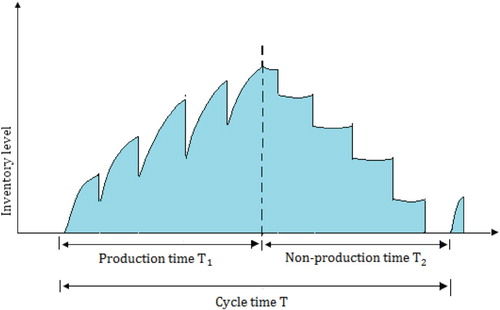
In our proposed scenario, a supplier delivers fixed quantities of a product to a buyer's warehouse at fixed time intervals. Each of these deliveries arrives at the warehouse at the exact time when all items from the previous delivery have just been depleted. Figures and demonstrate the inventory versus time for the buyer and the supplier. The total cycle time T can be divided into two components: , the time during which the supplier produces product and
, the time during which the supplier does not produce the product. Also we let
be the time between two successive deliveries. Under the assumptions described above, Yan et al. [Citation5] presented an integrated production-distribution inventory model for a deteriorating item with the assumption of constant deterioration. They derived the following average total cost which is sum of fixed setup cost, holding cost for suppler and buyer, deterioration cost for suppler and buyer, ordering cost, transportation and handling cost. Mathematically, the problem is given by
(2)
(2)
Figure 1. The buyer's inventory level versus time.
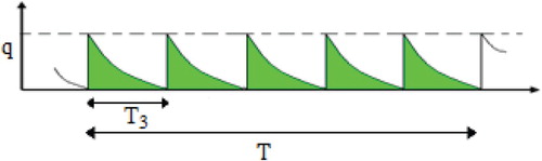
Figure 2. The supplier's inventory level versus time.
In real world applications, the deterioration rate in the inventory system may not be known precisely due to some uncontrollable factors. To incorporate this reality, we now attempt to modify model (2) by fuzzifying the deteriorating rate. Fuzzy sets representing linguistic concepts such as low, medium, high, etc., are employed to define states of a variable. Therefore, for any and
, we may remodify the average total cost function (as given in Equation (2)) as follows:
(3)
(3)
Note that in above model, the deteriorating rate during the planning horizon is assumed to be a fixed constant. However, when the inventory planning is completed, due to various uncertainties the deteriorating rate in practical problem may be not equal to
but just close to it. Therefore, it is difficult for the decision maker to determine a fixed value
for the deterioration rate in the planning horizon.
On the contrary, it is easier to set the deterioration rate in the interval where
and
are determined by the decision-maker. To find the corresponding fuzzy set with this interval
, we take any value
from this interval and then compare it with
of crisp value. If
, then we define the error
= 0. In the fuzzy sense, we can use the term confidence level instead of error. When the error is zero the confidence level will be the largest, and we set it to be 1. If
is located in
or
the farther the value
deviates from
, the larger of the error
, and hence, the smaller the confidence level. When
and
, the error
will attain to the largest, and the confidence level will be the smallest and we set it be zero. Therefore, corresponding to the interval
we set the triangular fuzzy number, ,
,
, because triangular fuzzy number is easy to handle. Moreover, the triangular fuzzy numbers may be used to model many kinds of uncertainties in this field of study. The pictorial sees Figure .
Figure 3. Triangular fuzzy number .
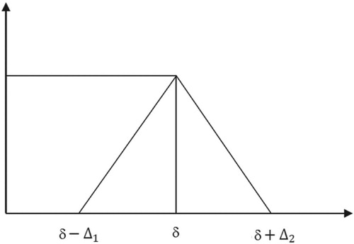
The membership grade of in
is 1. The farther the point in
is from both sides of d, the less the membership grade is. The membership grade shares the same property with the confidence level. If we make a correspondence between membership grade and confidence level, it is reasonable to set a fuzzy number in corresponding to the interval
. Further, here we describe the membership function of as follows:
(4)
(4)
Remark 4.1:
Centroid or centre of gravity method obtains the centre of area occupied by the fuzzy sets. It is given by the following formula
where
is membership function.
Hence, using the centre of gravity method, we can calculate the centroid for is given by
(5)
(5)
We regard this value as the estimate of deterioration rate in the fuzzy sense. Now, for any and
, we let
. Based on the extension principle (as expressed in Equation (1)), the membership function of the fuzzy average total cost
can be defined as
(6)
(6)
From
and Equation (3), we get
Hence,
(7)
(7)
Therefore, from Equations (4) and (7), the membership function of
can be written as
(8)
(8)
where
and
The pictorial of the membership function of
is shown in Figure . Now we can derive the centroid of
using Equation (5) as follows:
Figure 4. Triangular fuzzy number.
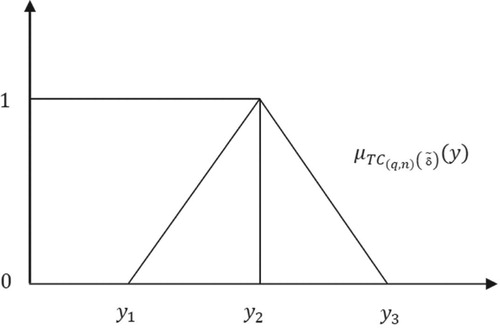
Accordingly, we can establish the following property1.
Property 1:
For any and
, the estimate of fuzzy average total cost function in Equation (3) is
(9)
(9)
Remark 4.2:
If we let = , then from Equation (9) we obtain
, which implies
Note 1. If
, then Figure is an isosceles triangle and Equation (9) reduces to
Note 2. If
Note 3. If
5. Solution Procedure
In this study, the classical differential calculus optimisation technique is used to find the optimal solution of the above problem (10). Thus, initially, the search for the optimal shipment number is reduced to a search for a locally optimal solution since the estimate in Equation (10) is a convex function of
for fixed
, and its minimised at
(11)
(11)
In addition, since the estimate in Equation (10) is a convex function of
for fixed
the unique optimal value of
can be obtained by setting Equation (13) to zero as
(12)
(12)
where
.
Lemma 5.1.
For fixed , the estimate in
is a convex function of
.
Proof:
Taking the first and second partial derivatives of with respect to
, we have
and
Therefore, for fixed
, the estimate in
is a convex function of
.
This completes the proof of lemma 5.1.
Lemma 5.2.
For fixed , the estimate in
is a convex function of
.
Proof:
Taking the first and second partial derivatives of with respect to
, we can obtain
(13)
(13)
and
.
Therefore, for fixed , the estimate in
is a convex function of
.
This completes the proof of lemma 5.2.
In this study the classical differential calculus optimisation technique is used to find the optimal solution of the proposed model. We have proved in Lemma 5.1. and 5.2. that the total cost of the proposed model as expressed in Equation (10) is a convex function of decision variables and
by examining the second order sufficient conditions (SOSC). Based on the convexity behaviour of objective function with respect to the decision variables we frame an algorithm to find the optimal values for the lot size
and the number of deliveries
in one production cycle. The optimality of the proposed algorithm is illustrated through numerical example. Through numerical test, we show that the proposed algorithm give quite satisfactory solutions.
Algorithm
Step 1. Let
Step 2. Substituting the given value of N into Equation (12) evaluates q.
Step 3. Compute the corresponding
Step 4. Set
Step 5. If
Step 6. Set
6. Numerical and Sensitivity Analysis
In this section, a numerical and sensitivity analysis are given to prove the convergence and the optimality of the proposed algorithm.
6.1. Numerical Analysis
We use the same data as in Yan et al. [Citation12] to demonstrates the difference of crisp and fuzzy case: ,
,
,
,
per production run,
,
,
,
. Here, we consider three cases:
. We solve each case for deterioration rate
. The results of the solution procedure are given in Table and the optimality of the proposed algorithm for the given example is shown in Figure . All the test problems are solved on a personal computer with Intel core i3-2100 processor having 3.10 GHz CPU and 4 Gig RAM. Furthermore, the algorithm is coded using the MATLAB 7.6.0.324 software.
Figure 5. Optimality of the algorithm for the given example. (a) Effects of D on average total cost (b) Effects of P on average total cost; (c) Effects of Hs on average total cost (d) Effects of Hb on average total cost; (e) Effects of C on average total cost (f) Effects of A on average total cost; (g) Effects of F on average total cost (h) Effects of Cd on average total cost.
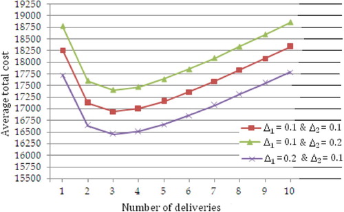
Table 1. Solution procedure of the model.
From Table , when (in this situation, the fuzzy case becomes the crisp case), by comparing
, we obtain the optimal solution
and the minimum estimate of fuzzy average total cost
, which are the same as shown in Yan et al. [Citation12]. In addition, when
and
, i.e. the fuzzy number
, we have
and
. Note that since
is the corresponding minimum average total cost in the crisp case, and hence the absolute relative variation in the fuzzy sense for the minimum average total cost is
Similarly, for the case and
, i.e. the fuzzy number
, we have
and
, and the absolute relative variation in the fuzzy sense for the minimum average total cost is
The results of Table show that the proposed algorithm converge at the point for the given example. We used the trial and error method to find the optimal values of
and N. However, we can easily observe that
is an optimal point of the given example because if we put the optimal value
in Equation (11), we can obtain the optimal value
. Accordingly, Table and Figure indicate that the proposed algorithm should converge.
6.2. Sensitivity Analysis
We now study the effects of parameters ,
,
,
,
,
and
in order to illustrate the difference of crisp and fuzzy case and, to prove the convergence and the optimality of the proposed algorithm. The sensitivity analysis is performed by changing the parameters of
,
,
,
,
,
and
by +50%, +25%, −25% and −50%. The results of the sensitivity analysis are shown in Tables and the corresponding curves of average total cost are shown in Figure . Tables establish the optimality and converge of the proposed algorithm.
Figure 6. Percentage changes of parameters on the average total cost.
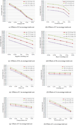
Table 2. Effects of on optimal solution.
Table 3. Effects of on optimal solution.
Table 4. Effects of on optimal solution.
Table 5. Effects of on optimal solution.
Table 6. Effects of on optimal solution.
Table 7. Effects of on optimal solution.
Table 8. Effects of on optimal solution.
7. Conclusion
Successful inventory system is recognised as a crucial activity to increase operational effectiveness across high competitive business, to improve customer service, and to reduce inventory costs at different locations of a supply network. Today's one of the most important aspects of inventory management that has significant role in supply chain operations is the deterioration of products in multi-echelon inventory systems. In real-world applications, the deterioration rate in the inventory system may not be known precisely due to some uncontrollable factors. In other words, the probability distribution of the deterioration rate is typically unknown because of a lack of historical information, and the use of linguistic expressions by experts for deterioration rate forecasting is often employed. Therefore, the decision maker faces a fuzzy deterioration environment rather than a stochastic one. Several researches reveal that the decision variables and the total cost are sensitive to the level of fuzziness in the input parameters. Hence, the practitioner and /or decision maker is advised to be more careful in accounting flexibility in the input parameters. In view of this, this research proposed an optimisation inventory policy for a deteriorating with fuzzy deterioration rate and the supplier's production batch size is restricted to an integer multiple of the delivery lot quantity to the buyer.
Disclosure statement
No potential conflict of interest was reported by the author(s).
Additional information
Notes on contributors
S. Priyan
S. Priyan is currently an Assistant Professor (Sl. Grade) in the Department of Mathematics at Hindustan Institute of Technology & Science (Deemed be to be University), Chennai, India. He received his PhD in Mathematics from The Gandhigram Rural Institute (Deemed to be University), Gandhigram, India in 2015. He has published about 29 papers in international reputed journals. His research interests include the following fields: operations research and industrial engineering.
P. Mala
P. Mala is a research scholar in the Department of Mathematics at Mepco Schlenk Engineering College, Sivakasi, India. Her Ph.D. research area is Inventory analysis and she published more than 4 papers in reputed journals.
References
- Chang CT, Ouyang LY, Teng JT, et al. Optimal ordering policies for deteriorating items using a discounted cash-flow analysis when a trade credit is linked to order quantity. Comput Ind Eng. 2010;59:770–777.
- Yang PC, Wee HM. A single-vendor and multiple-buyers production–inventory policy for a deteriorating item. Eur J Oper Res. 2002;143:570–581.
- Yang PC, Wee HM. An integrated multi-lot-size production inventory model for deteriorating item. ComputOper Res. 2003;30:671–682.
- Chung CJ, Wee HM. An integrated production-inventory deteriorating model for pricing policy considering imperfect production, inspection planning and warranty-period and stock-level-dependant demand. Int J Syst Sci. 2008;39:823–837.
- Yan C, Banerjee A, Yang L. An integrated production-distribution model for a deteriorating inventory item. Int J Prod Econ. 2011;133:228–232.
- Sarkar B. A production-inventory model with probabilistic deterioration in two-echelon supply chain management. Appl Math Model. 2013;37:3138–3151.
- Lee S, Kim D. An optimal policy for a single-vendor single-buyer integrated production–distribution model with both deteriorating and defective items. Int J Prod Econ. 2014;147:161–170.
- Rout C, Paul A, Kumar RS, et al. Cooperative sustainable supply chain for deteriorating item and imperfect production under different carbon emission regulations. J Clean Prod. 2020;272:122170.
- Anil KA, Susheel Y. Price and profit structuring for single manufacturer multi-buyer integrated inventory supply chain under price-sensitive demand condition. Comput Ind Eng. 2020;139:106208.
- Zadeh L. Fuzzy sets. Inf Control. 1965;8:338–353.
- Ishii H, Konno TA. A stochastic inventory problem with fuzzy shortage cost. Eur J Oper Res. 1998;106:90–94.
- Yao JS, Lee HM. Fuzzy inventory with or without backorder for fuzzy order quantity with trapezoid fuzzy number. Fuzzy Sets Syst. 1999;105:311–337.
- Yao JS, Chiang J. Inventory without backorder with fuzzy total cost and fuzzy storing cost defuzzified by centroid and signed distance. Eur J Oper Res. 2003;148:401–409.
- Roy A, Maiti MK, Kar S, et al. Two storage inventory model with fuzzy deterioration over a random planning horizon. Math Comput Model. 2007;46:1419–1433.
- Mishra N, Soni JK. An EOQ inventory model with fuzzy deterioration rate and finite production rate. IOSR J Math. 2012;4:1–9.
- Liu ST. Solution of fuzzy integrated production and marketing planning based on extension principle. Comput Ind Eng. 2012;63:1201–1208.
- Shabani S, Mirzazadeh A, Sharifi E. An inventory model with fuzzy deterioration and fully backlogged shortage under inflation. Sop Trans Appl Math. 2014;1:161–171.
- Pu PM, Liu YM. Fuzzy topology. I. Neighborhood structure of a fuzzy point and Moore-Smith convergence. J Math Anal Appl. 1980;76:571–599.
- Chiang J, Yao JS, Lee HM. Fuzzy inventory with backorder defuzzification by signed distance method. J Inf Sci Eng. 2005;21:673–694.