A New Method for Optimal Solution of Intuitionistic Fuzzy Transportation Problems via Generalized Trapezoidal Intuitionistic Fuzzy Numbers

Abstract

In this paper, we introduce the new method for solving the intuitionistic fuzzy transportation problem (IFTP), by using north-west corner method and modified distribution method to find the optimal solution for IFTP.

KEYWORDS:

• Intuitionistic fuzzy set
• matrix game
• linear programming
• intuitionistic fuzzy transportation problem

1. Introduction

In 1956, Zadeh [1] firstly defined the concept of fuzzy set theory. The concept of an intuitionistic fuzzy set was proposed by Atanassov in 1986 [2]. This concept referred to the reflection of the relation among ‘1 minus the degree of membership’, ‘the degree of non-membership’ and ‘the degree of hesitation’. The intuitionistic fuzzy set was rasterised by the degree of membership and the degree of non-membership. The intuitionistic fuzzy set had more abundant and flexible than the fuzzy set with uncertain information. Many researchers have also used fuzzy and intuitionistic fuzzy set for solving real world optimisation problems such as transportation problem.

The transportation problem is a special kind of optimisation problem. Transportation problem is interested in finding the least total transportation cost of goods in order to satisfy demand at destinations using available supplies at the sources. In usual, transportation problems are solved with the hypothesis that values of supplies and demands and the transportation costs are specified in a precise way. In the real world, in many cases, the decision-maker has no crisp information about the coefficients belonging to the transportation problem. In this situation, the corresponding elements defining the problem can be formulated by mean of fuzzy set, and the fuzzy transportation problem appears in a natural way. In 1941, Hitchcock [3] originally developed the basic transportation problem. Dantzig [4] applied linear programming to solving the transportation problem. Several authors have carried out an examination about fuzzy transportation problem [5–9]. Moreover, several authors have used intuitionistic fuzzy set theory for solving transportation problems. Hussain and Kumar [10] investigate the transportation problem with the aid of triangular intuitionistic fuzzy numbers (TIFN). Pramila and Uthra [11] presented optimal solution of an IFTP. Antony et al. [12] studied method for solving the transportation problem by using TIFN. Singh and Yadav [13] discussed new approach for solving IFTP of type-2 where the supply, demand are fixed crisp numbers and the cost is TIFN.

In this paper, we using a linear ranking function for generalised trapezoidal intuitionistic fuzzy numbers (GTrIFNs) to find the IBFS and optimal solution of GTrIFNs based on the allocation of demands and availabilities are real numbers and cots are GTrIFNs. This paper is organised as follows. Section 2 gives the concept of mathematics preliminaries. Section 3 presents ranking of GTrIFN. Section 4 describes a mathematics formulation for IFTP. Section 5 details some numerical example. In the final section, the paper is concluded in Section 6.

2. Mathematical Preliminaries

In this section, we give some basic definitions and concepts of cut sets of trapezoidal intuitionistic fuzzy number (TrIFN).

2.1. Some Definitions of TrIFNs

Definition 2.1

[1]: Let $X$ be an arbitrary nonempty set of the universe. A fuzzy set $A$ in $X$ is a function with domain X and values in $\left[0,1\right].$ If A is a fuzzy set and $x\in X$, then the function value ${\mu }_A\left(x\right)$ is called the membership function of x in A. A fuzzy set can be written as order pair, given by $\left\{x,{\mu }_A\left(x\right)\mid x\in X\right\}$ where $0\le {\mu }_A\left(x\right)\le 1.$

Definition 2.2

[2]: Let $X$ be an arbitrary nonempty set of the universe. If there are two mapping on the set X: ${\mu }_A\left(x\right):X\to \left[0,1\right]$ and ${\nu }_A\left(x\right):X\to \left[0,1\right]$ with the condition 0 ≤${\mu }_A\left(x\right)$ + ${\nu }_A\left(x\right)$≤ 1. The ${\mu }_A$ and ${\nu }_A$ are called determining and intuitionistic fuzzy set A on the universal set $X$, denote by $\left\{x;{\mu }_A\left(x\right),{\nu }_A\left(x\right)\mid x\in X\right\}$ we called ${\mu }_A$ and ${\nu }_A$ are membership function and nonmembership function of A, respectively. ${\mu }_A\left(x\right)$ and ${\nu }_A\left(x\right)$ are called the membership degree and nonmembership degree of an element x belonging to $A\subseteq X$, respectively. $IF\left(X\right)$ is called the set of the intuitionistic fuzzy set on the universal set $X.$

Definition 2.3:

An intuitionistic fuzzy number (IFN) A is

1. subset of the real line.

2. convex for the membership function ${\mu }_A\left(x\right),$ that is, ${\mu }_A\left(\alpha x_1+\left(1-\alpha \right)x_2\right)\ge min\left({\mu }_A(x_1\right),{\mu }_A\left(x_2\right))\text{ for all }{x}_1,x_2\in \mathbb{R},\alpha \in [0,1]$

3. concave for the non-membership function ${\nu }_A\left(x\right),$ ${\nu }_A\left(\alpha x_1+\left(1-\alpha \right)x_2\right)\le max\left({\nu }_A\right(x_1),{\nu }_A(x_2\left)\right)\text{ for all }{x}_1,x_2\in \mathbb{R},\alpha \in \left[0,1\right]$

4. normal, that is, ${\mu }_A\left(x_0\right)=1,{\nu }_A\left(x_0\right)=0$ for some $x_0\in \text{ R}$.

Definition 2.4:

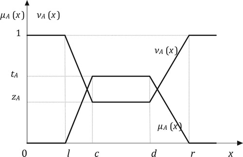
A TrIFN $A=\left(l,c,d,r\right);t_A,z_A$ is called GTrIFN, is shown Figure 1 if its membership and nonmembership functions are defined as follows: (1) ${\mu }_A\left(x\right)=\left\{\begin{array}{ll}0& \text{if }x<l\\ t_A\left(x-l\right)/\left(c-l\right)& \text{if }l\le x<c\\ t_A& \text{if }c\le x\le d\\ t_A\left(r-x\right)/\left(r-d\right)& \text{if }d<x\le r\\ 0& \text{if }x>r\end{array}\right.$(1)

And (2) ${\nu }_A\left(x\right)=\left\{\begin{array}{ll}1& \text{if }x<l\\ \left[c-x+z_A\left(x-l\right)\right]/\left(c-l\right)& \text{if }l\le x<c\\ z_A& \text{if }c\le x\le d\\ \left[x-d+\frac{z_A\left(r-x\right)}{r-d}\right]& \text{if }d<x\le r\\ 1& \text{if }x>r\end{array}\right.$(2) respectively, where $l\le c\le d\le r,$ the values $t_A$ and $z_A〈sub〉〈/sub〉$ are maximum membership degree and minimum nonmembership degree of A, respectively, such that they satisfy the following condition: $t_A\in \left[0,1\right],z_A\in \left[0,1\right]and{t}_A+z_A\in \left[0,1\right]$.

Let (3) ${\pi }_A\left(x\right)=1-{\mu }_A\left(x\right)-{\nu }_A\left(x\right)$(3) ${\pi }_A\left(x\right)$ is called the hesitancy degree of an element $x\in A$. It is the degree of indeterminacy membership of the element $x$ to $A$.

Figure 1. A TrIFN $A=\left(l,c,d,r\right);t_A,z_A$.

From Definition 2.4, it is obvious that ${\mu }_A\left(x\right)+{\nu }_A\left(x\right)=1$ for any $x\in R$ if $t_A=1$ and $z_A=0$. Hence, the TrIFN $A=\left(l,c,d,r\right);t_A,z_A$ degenerates to $A=\left(l,c,d,r\right);1,0$, which is a trapezoidal fuzzy number (TrFN) [14]. Therefore, the concept of the TrIFN is generalisation of that of the TrFN.

From $A=\left(l,c,d,r\right);t_A,z_A$ if $c=d=p$ then $A=\left(l,p,r\right);t_A,z_A$ that is $A=\left(l,p,r\right);t_A,z_A$ is a TIFN, which is particular case of TrIFN. Likewise to algebraic operations of TIFN and TrIFN are defined as follows.

Definition 2.5:

Let $A=\left(l_1,c_1,d_1,r_1\right);t_A,z_A$ and $B=\left(l_2,c_2,d_2,r_2\right);t_B,z_B$ be two GTrIFNs with $t_A\ne t_B,z_A\ne z_B\text{ and }\gamma \ne 0$ be any real number. Then, the algebraic operations of GTrIFNs are defined as follows: $\begin{array}{rl}A\oplus B& =\left(l_1+l_2,c_1+c_2,d_1+d_2,r_1+2_2\right);t_A\wedge t_B,z_A\vee z_B\end{array}$ $\begin{array}{rl}A\ominus B& =\left(l_1-r_2,c_1-d_2,d_1-c_2,r_1-l_2\right);t_A\wedge t_B,z_A\vee z_B\end{array}$ $\begin{array}{rl}A\otimes B& =\left\{\begin{array}{ll}\left(l_1{l}_2,c_1{c}_2,d_1{d}_2,r_1{r}_2\right);t_A\wedge t_B,z_A\vee z_B& \text{ if }A>0,B>0\\ \left(l_1{r}_2,c_1{d}_2,d_1{c}_2,r_1{l}_2\right);t_A\wedge t_B,z_A\vee z_B& \text{ if }A〈0,B〉0\\ \left(r_1{r}_2,d_1{d}_2,c_1{c}_2,l_1{l}_2\right);t_A\wedge t_B,z_A\vee z_B& \text{ if }A<0,B<0\end{array}\right.\end{array}$ $\begin{array}{rl}A\oslash B& =\left\{\begin{array}{ll}\left(l_1/r_2,c_1/d_2,d_1/c_2,r_1/l_2\right);t_A\wedge t_B,z_A\vee z_B& \text{ if }A>0,B>0\\ \left(r_1/r_2,d_1/d_2,c_1/c_2,l_1/l_2\right);t_A\wedge t_B,z_A\vee z_B& \text{ if }A〈0,B〉0\\ \left(r_1/l_2,d_1/c_2,c_1/d_2,l_1/r_2\right);t_A\wedge t_B,z_A\vee z_B& \text{ if }A<0,B<0\end{array}\right.\end{array}$ $\begin{array}{rl}\gamma A& =\left\{\begin{array}{cc}\left(\gamma l_1,\gamma c_1,\gamma d_1,\gamma r_1\right);t_A,z_A& \text{ if }\gamma >0\\ \left(\gamma r_1,\gamma d_1,\gamma c_1,\gamma l_1\right);t_A,z_A& \text{ if }\gamma <0\end{array}\right.\end{array}$ $\begin{array}{rl}{A}^{\ast -1}& =\left(1/r_1,1/d_1,1/c_1,1/l_1\right);t_A,z_A\text{ if }A\ne 0\end{array}$ where the symbols ∧ is the minimum operator and ∨ is the maximum operator.

2.2. Cut Sets of TrIFN

Definition 2.6

[15]: A $\left(\alpha ,\lambda \right)-$ cut set of $A=\left(l,c,d,r\right);t_A,z_A$ is a crisp subset of R, which is defined as follows: $A_{\alpha }^{\ast \lambda }=\left\{x|{\mu }_A\right(x)\ge \alpha ,{\nu }_A(x)\le \lambda \}$ where $0\le \alpha \le t_A,z_A\le \lambda \le 1$ and $0\le \alpha +\lambda \le 1$.

Definition 2.7

[15]: The $\alpha -$ cut set and $\lambda$-cut set of $A=\left(l,c,d,r\right);t_A,z_A$ are a crisp subset of R, which is defined as follows: $A_{\alpha }=\left\{x|{\mu }_A\right(x)\ge \alpha \}$ and $A^{\ast \lambda }=\left\{x|{\nu }_A\right(x)\le \lambda \}$ respectively.

Using the membership function of $A=\left(l,c,d,r\right);t_A,z_A$ and Definition 2.7 such that $A_{\alpha }=\left\{x|{\mu }_A\right(x)\ge \alpha \}$ and $A^{\ast \lambda }=\left\{x|{\nu }_A\right(x)\le \lambda \}$ are closed interval and calculated as follows: (10) $A_{\alpha }=\left[L_A\left(\alpha \right),R_A\left(\alpha \right)\right]=\left[\frac{\left(t_A-\alpha \right)l+\alpha c}{t_A},\frac{\left(t_A-\alpha \right)r+\alpha d}{t_A}\right]$(10) and (11) $A^{\lambda }=\left[L_A^{{}^{\mathrm{\prime }}}\left(\lambda \right),R_A^{{}^{\mathrm{\prime }}}\left(\lambda \right)\right]=\left[\frac{\left(1-\lambda \right)c+\left(\lambda -z_A\right)l}{1-z_A},\frac{\left(1-\lambda \right)d+\left(\lambda -z_A\right)r}{1-z_A}\right]$(11) respectively.

3. Ranking of TrIFN

This section briefly reviews the ambiguities and the accuracy function of a GTrIFN.

Definition 3.1:

Let $A$ be an arbitrary IFN. The score function for the IFN $A$ for membership and non-membership functions are denoted by $M\left({\mu }_A\right)$ and $M\left({\nu }_A\right),$respectively. $M\left({\mu }_A\right)$ and $M\left({\nu }_A\right)$ are defined by (12) $M\left({\mu }_A\right)={\int }_0^{t_A}\left[L_A\left(\alpha \right)+R_A\left(\alpha \right)\right]h\left(\alpha \right)d\left(\alpha \right)$(12) and (13) $M\left({\nu }_A\right)={\int }_{z_A}^1\left[L_A^{{}^{\mathrm{\prime }}}\left(\lambda \right)+R_A^{{}^{\mathrm{\prime }}}\left(\lambda \right)\right]g\left(\lambda \right)d\left(\lambda \right)$(13)

where $h\left(\alpha \right)$ and $g\left(\lambda \right)$ satisfy the following conditions:

1. h(α) and g(λ) are monotonic increasing of $\alpha \in \left[0,t_A\right]$ and monotonic decreasing of$\lambda \in \left[z_A,1\right]$.

2. $h\left(\alpha \right)\in \left[0,1\right]$ and $g\left(\lambda \right)\in \left[0,1\right].$ (iii) $h\left(0\right)=0$ and $g\left(1\right)=0$.

Let $A$ be an arbitrary IFN. The ambiguities for IFN $A$ for membership and nonmembership functions are denote by V (µ_A) and V (ν_A), respectively. respectively. $V\left({\mu }_A\right)$ and $V\left({\nu }_A\right)$ are defined by (14) $V\left({\mu }_A\right)={\int }_0^{t_A}\left[L_A\left(\alpha \right)+R_A\left(\alpha \right)\right]h\left(\alpha \right)d\left(\alpha \right)$(14) and (15) $V\left({\nu }_A\right)={\int }_{z_A}^1\left[L_A^{{}^{\mathrm{\prime }}}\left(\lambda \right)+R_A^{{}^{\mathrm{\prime }}}\left(\lambda \right)\right]g\left(\lambda \right)d\left(\lambda \right)$(15) Next, we find score, accuracy and ambiguities function of a GTrIFN.

Let a GTrIFN $A=\left(l,c,d,r\right);t_A,z_A$ the score function of a GTrIFN A for membership and non-membership functions can be written as follows: from Equations (10), (12) and $h\left(\alpha \right)=\alpha$, we get (16) $M\left({\mu }_A\right)=\frac{l+2c+2d+r}{6}{t}_A^2$(16) Similarly, from Equations (11), (13) and $g\left(\lambda \right)=\lambda ,$ we have (17) $M\left({\nu }_A\right)=\frac{l+2c+2d+r}{6}(1-z_A{)}^2$(17) The accuracy function of a GTrIFN $A$ is denoted by (18) $\begin{array}{r}\mathrm{\Delta }\left(A\right)=\frac{M\left({\mu }_A\right)+M\left({\nu }_A\right)}{2}=\frac{\left(l+2c+2d+r\right)t_A^2+\left(l+2c+2d+r\right){\left(1-z_A\right)}^2}{12}\end{array}$(18) from Equations (10), (14) and $h\left(\alpha \right)=\alpha ,$ we get (19) $V\left({\mu }_A\right)=\frac{r-l+2d-2c}{6}{t}_A^2$(19) Similarly, from Equations (11), (15) and $g\left(\lambda \right)=\lambda$, we get (20) $V\left({\nu }_A\right)=\frac{r-l+2d-2c}{6}(1-z_A{)}^2.$(20) The accuracy function of a GTrIFN $A$ is denoted by (21) $\mathrm{\nabla }\left(A\right)=\frac{V\left({\mu }_A\right)+V\left({\nu }_A\right)}{2}=\frac{\left(r-l+2d-2c\right)t_A^2+\left(r-l+2d-2c\right){\left(1-z_A\right)}^2}{12}.$(21)

Example 3.1:

Let $A=〈\left(155,165,175,180\right);0.7,0.2〉$and $B=〈\left(130,146,150,165\right);0.6,0.3〉$ be two GTrIFNs then, $\begin{array}{rl}M\left({\mu }_A\right)& =\frac{\left(155+2\left(165\right)+2\left(175\right)+180\right){\left(0.7\right)}^2}{6}=82.892\\ M\left({\nu }_A\right)& =\frac{\left(155+2\left(165\right)+2\left(175\right)+180\right){(1-0.2)}^2}{6}=108.267\\ \therefore \mathrm{\Delta }\left(A\right)& =\frac{82.892+108.267}{2}=95.580\\ V\left({\mu }_A\right)& =\frac{\left(180-155+2\left(175\right)-2\left(165\right)\right){\left(0.7\right)}^2}{6}=3.675\\ V\left({\nu }_A\right)& =\frac{\left(180-155+2\left(175\right)-2\left(165\right)\right){(1-0.2)}^2}{6}=4.8\\ \therefore \mathrm{\nabla }\left(A\right)& =\frac{3.675+4.8}{2}=4.328\\ M\left({\mu }_B\right)& =\frac{\left(130+2\left(146\right)+2\left(150\right)+165\right){\left(0.6\right)}^2}{6}=8.87\\ M\left({\nu }_B\right)& =\frac{\left(130+2\left(146\right)+2\left(150\right)+165\right){(1-0.3)}^2}{6}=72.438\\ \therefore \mathrm{\Delta }\left(B\right)& =\frac{8.87+72.438}{2}=40.65\\ V\left({\mu }_B\right)& =\frac{\left(165-130+2\left(150\right)-2\left(146\right)\right)){\left(0.6\right)}^2}{6}=2.58\\ V\left({\nu }_B\right)& =\frac{\left(165-130+2\left(150\right)-2\left(146\right)\right)){(1-0.3)}^2}{6}=3.512\\ \therefore \mathrm{\nabla }\left(B\right)& =\frac{2.58+3.512}{2}=3.046\end{array}$

Theorem 3.1:

Let $A=\left(a_1,a_2,a_3,a_4\right);t_A,z_A$ and $B=\left(b_1,b_2,b_3,b_4\right);t_B,z_B$ be GTrIFNs with $t_A=t_B$ and $z_A=z_B.$ The accuracy function $\mathrm{\Delta }:GIF\left(R\right)\to R$ is a linear function.

Proof:

Let$A=\left\{\left(a_1,a_2,a_3,a_4\right);t_A,z_A\right\}$ and $B=\left\{\left(b_1,b_2,b_3,b_4\right);t_B,z_B\right\}$ then $\gamma \ge 0,\text{β}\ge 0$, we have $\begin{array}{rl}& \Delta ({\gamma }_A+{\text{β}}_B)\\ & =\Delta \left\{\left(\gamma a_1,\gamma a_2,\gamma a_3,\gamma a_4\right);t_A,z_A\right\}+\left\{\left(\text{β}{b}_1,\text{β}{b}_2,\text{β}{b}_3,\text{β}{b}_4\right);t_B,z_B\right\}\\ & =\Delta \left\{\left\{\left(\gamma a_1+\text{β}{b}_1,\gamma a_2+\text{β}{b}_2,\gamma a_3+\text{β}{b}_3,\gamma a_4+\text{β}{b}_4\right);t_A\wedge t_B,z_A\vee z_B\right\}\right\}\\ & =\frac{1}{12}\left\{\right\{(\gamma a_1+\text{β}{b}_1)+2(\gamma a_2+\text{β}{b}_2)+2(\gamma a_3+\text{β}{b}_3)\\ & +(\gamma a_4+\text{β}{b}_4)\left){(t_A\wedge t_B)}^2\right\}\}+\frac{1}{12}\{\left\{\right(\gamma a_1+\text{β}{b}_1)+2(\gamma a_2+\text{β}{b}_2)\\ & +2(\gamma a_3+\text{β}{b}_3)+(\gamma a_4+\text{β}{b}_4)\left)\right(1-{(z_A\vee z_B)}^2\left\}\right\}\\ & =\frac{1}{12}\left\{\left\{\left(\gamma a_1+2\gamma a_2+2\gamma a_3+\gamma a_4)+(\text{β}{b}_1+2\text{β}{b}_2+2\text{β}{b}_3+\text{β}{b}_4)\right)){(t_A\wedge t_B)}^2\right\}\right\}\\ & +\frac{1}{12}\left\{\left\{\left(\gamma a_1+2\gamma a_2+2\gamma a_3+\gamma a_4\left)+\right(\text{β}{b}_1+2\text{β}{b}_2+2\text{β}{b}_3+\text{β}{b}_4)\right)\left)\right(1-{(z_A\vee z_B)}^2\right\}\right\}\\ & =\gamma \left(\frac{1}{12}\left(a_1+2a_2+2a_3+a_4\right){\left(t_A\right)}^2\right)+\text{β}\left(\frac{1}{12}\left(b_1+2b_2+2b_3+b_4\right){\left(t_B\right)}^2\right)\\ & +\gamma \left(\frac{1}{12}\left(a_1+2a_2+2a_3+a_4\right){\left(1-z_A\right)}^2\right)+\text{β}\left(\frac{1}{12}\left(b_1+2b_2+2b_3+b_4\right){\left(1-z_B\right)}^2\right)\\ & =\gamma \left(\frac{1}{12}\left(a_1+2a_2+2a_3+a_4\right){\left(t_A\right)}^2+\left(a_1+2a_2+2a_3+a_4\right){\left(1-z_A\right)}^2\right)\\ & +\text{β}\left(\frac{1}{12}\left(b_1+2b_2+2b_3+b_4\right){\left(t_B\right)}^2+\left(b_1+2b_2+2b_3+b_4\right){\left(1-z_B\right)}^2\right)\\ & =\gamma \Delta \left(A\right)+\text{β}\Delta \left(B\right).\end{array}$ In the same way, if $\gamma <0,\text{β}<0$ we can prove $\mathrm{\Delta }\left(\gamma A+B\right)=\gamma \mathrm{\Delta }\left(A\right)+\mathrm{\Delta }\left(B\right).$

Therefore,$\mathrm{\Delta }$ is a linear function.

Theorem 3.2:

Let$A=\left(a_1,a_2,a_3,a_4\right);t_A,z_A\text{ and }B=\left(b_1,b_2,b_3,b_4\right);t_B,z_B$ be GTrIFNs with $t_A=t_B$ and $z_A=z_B.$ The ambiguities function $\mathrm{\Delta }:GIF\left(R\right)\to R$ is a linear function.

(The rest of the proof is similar to proof of Theorem 3.1).

Definition 3.2:

Let $A=\left(a_1,a_2,a_3,a_4\right);t_A,z_A\text{ and }B=\left(b_1,b_2,b_3,b_4\right);t_B,z_B$ be GTrIFNs. The ranking order of $A\text{and}B$ is stipulated as follows:

1. if $\mathrm{\Delta }A>\mathrm{\Delta }B,thenA>B$

2. if $\mathrm{\Delta }A<\mathrm{\Delta }B,thenA<B$

3. if $\mathrm{\Delta }A=\mathrm{\Delta }B,$ then

   1. if $\mathrm{\nabla }\left(A\right)=\mathrm{\nabla }\left(B\right),thenA=B$

   2. if $\mathrm{\nabla }\left(A\right)>\mathrm{\nabla }\left(B\right),thenA<B$

   3. if $\mathrm{\nabla }\left(A\right)〈\mathrm{\nabla }\left(B\right),thenA〉B$

4. Mathematical Formulation for IFTP

This section, first introduces the mathematical formulation of the IFTP. Later, we find IBFS by NWCM and we use MODIM for finding optimal solution. The mathematical formulation of the IFTP is of the following form: $\begin{array}{rl}& \left(\text{IFTP:1}\right)\text{ Minimize }\mathrm{\Psi }=\sum _{i=1}^m\sum _{j=1}^n{c}_{i,j}{x}_{i,j}\\ & \text{subject to}\\ & \sum _{j=1}^n{x}_{ij}\le a_i,i\in \left\{1,2,\dots ,m\right\}\\ & \sum _{i=1}^m{x}_{ij}\ge b_j,j\in \left\{1,2,\dots ,n\right\}\\ & x_{ij}\ge 0\text{ for all }i\text{ and }j\end{array}$ where $c_{ij}$ be GTrIFN cost of transportation one unit of the goods from $i^{th}$ source to the $j^{th}$ destination. $x_{ij}$ be the quantity transportation from $i^{th}$ source to the $j^{th}$ destination, is shown Table 1.

Here, $a_i$ be the total availability of the goods at $i^{th}$source.

$b_i$ be the total demand of the goods at $j^{th}$destination.

$\sum _{i=1}^m\sum _{j=1}^n{x}_{ij}{c}_{ij}$ be total intuitionistic fuzzy transportation cost.

If $\sum _{i=1}^m{a}_i=\sum _{j=1}^n{b}_j$ then IFTP is said to be balanced.

If $\sum _{i=1}^m{a}_i\ne \sum _{j=1}^n{b}_j$ then IFTP is said to be unbalanced (Table 1).

Table 1. The intuitionistic fuzzy transportation table.

	1	2	…	N	$a_i$
1	$c_{11}$	$c_{12}$	…	$c_{1n}$	$a_1$
2	$c_{21}$	$c_{22}$	…	$c_{2n}$	$a_2$
…	…	…	…	…	…
$b_j$	$b_1$	$b_2$	…	$b_n$	$\sum _{i=1}^m{a}_i=\sum _{j=1}^n{b}_j$

From IFTP:1 can be written as the following linear programming problem (LPP): Minimize $\begin{array}{rl}\text{(LPP): Minimize}\mathrm{\Psi }\left(X\right)& =C^T\left(X\right)\\ \text{subject to}AX& =b\\ X& \ge 0,\end{array}$ where $A$ be an $m\times n$ matrix, $X$ be an n − vector, $b$ be an m − vector, and $c=(c_{11},c_{12},\dots ,c_{1n},\dots ,c_{m1},\dots ,c_{mn}{)}^T$.

Theorem 4.1:

Let the intuitionistic fuzzy linear programming problem (IFLPP) be given as (22) $\begin{array}{ll}\text{Minimize}& \mathrm{\Psi }\left(X\right)=C^T\left(X\right)\\ \text{subject to}& AX=b\\ & X\ge 0,\end{array}$(22) where $A=(a_{ij}{)}_{m\times n}=\left(A_1,A_2,\dots ,A_n\right),c=\left(c_1,c_2,\dots ,c_n\right)\text{ and }b=(b_i{)}_{m\times 1},c_j,j=1,2,\dots ,n$ are GTrIFNs. If for BFS $X_B$, all ${\mathrm{\Psi }}_j=\sum _{j=1}^n(c_B{)}^T{B}^{-1}{A}_j,$ then $X_B$ is optimal solution, where $\mathrm{\Psi }j$ are given by ${\mathrm{\Psi }}_j=\sum _{j=1}^n(c_B{)}^T{B}^{-1}{A}_j\text{ and }{B}^{-1}{A}_j={\xi }^j.$

Proof:

We need to prove $\mathrm{\Psi }\left(X_B\right)\le \mathrm{\Psi }\left(Z\right).$ Let $c_B=\left(c_1,c_2,\dots ,c_m\right),B=\left(A_1,A_2,\dots ,A_m\right),X_B=\left(x_1,x_2,\dots ,x_m\right),$ $\mathrm{\Psi }\left(X_B\right)=C_B^T\left(X_B\right)$, where $x_i\left(i=1,2,\dots ,m\right),$ is some $x_j\left(j=1,2,\dots ,m\right),$. Let$\text{ Z}=\left(z_1,z_2,\dots ,z_m,\dots ,z_n\right),$ any other feasible solution with $z_i\left(i=1,2,\dots ,m,\dots ,,n\right)$ some $x_j\left(j=1,2,\dots ,m\right)$. Since $B$ is basis, we have (23) $A_j={\xi }_1^j{A}_1+{\xi }_2^j{A}_2+\cdots +{\xi }_m^j{A}_m,j\in \left\{1,2,\dots ,n\right\}$(23)

Also, Z is a feasible solution. This refer to (24) $z_1{A}_1+z_2{A}_2+\cdot \cdot \cdot +z_n{A}_n=b$(24) from Equations (23)and (24), we get $\left(z_1{\xi }_1^1+z_2{\xi }_1^2+\cdots +z_n{\xi }_1^n\right)A_1+\cdots +\left(z_1{\xi }_m^1+z_2{\xi }_m^2+\cdots +z_n{\xi }_m^n\right)A_m=b$ Since $XB$ is a solution, that is (26) $x_1{A}_1+x_2{A}_2+\cdot \cdot \cdot +x_n{A}_n=b$(26) Then Equations (25) and (26), together imply that $x_i=\sum _{j=1}^n{z}_i{\xi }_i^j,x_i\left(i=1,2,\dots ,m\right)$ Since $\mathrm{\Delta }\left(c_j\ominus {\mathrm{\Psi }}_j\right)\ge 0\mathrm{a}\mathrm{n}\mathrm{d}\mathrm{\Delta }$ is linear, therefore, $\begin{array}{rl}\mathrm{\Delta }\left(\mathrm{\Psi }\left(z\right)\right)& =\mathrm{\Delta }\left(c_1{z}_1\oplus c_2{z}_2\oplus \dots c_n{z}_n\right)\\ \ge & \mathrm{\Delta }\left({\mathrm{\Psi }}_1{z}_1\oplus {\mathrm{\Psi }}_2{z}_2\oplus \dots {\mathrm{\Psi }}_n{z}_n\right)\\ & =\mathrm{\Delta }\left(\sum _{j=1}^n{\left(c\right)}^T{\xi }^j{z}_j\right)\\ & =\sum _{j=1}^n\left(\mathrm{\Delta }\left(\sum _{i=1}^m{c}_i{\xi }_i^j\right)\right)z_j\\ & =\sum _{i=1}^m\mathrm{\Delta }\left(c_i\right)\sum _{j=1}^n{z}_j{\xi }_i^j\\ & =\sum _{i=1}^m\mathrm{\Delta }\left(c_i\right)x_i\\ & =\mathrm{\Delta }\left(\sum _{i=1}^m{c}_i{x}_i\right)\\ & =\mathrm{\Delta }\left(\mathrm{\Psi }\left(X_B\right)\right)\end{array}$ This implies that $\mathrm{\Delta }\left(\mathrm{\Psi }\left(X_B\right)\right)\le \mathrm{\Delta }\left(\mathrm{\Psi }\left(Z\right)\right)$ and therefore $\mathrm{\Psi }\left(X_B\right)\le \mathrm{\Psi }\left(Z\right).$ So,$X_B$ is optimal solution.

The dual of the IFTP:1 can be written as $\begin{array}{rl}& \text{Maximize }{\mathrm{\Psi }}_{\left(D\right)}=\sum _{i=1}^m{a}_i{u}_i\oplus \sum _{j=1}^n{b}_i{v}_j\\ & \text{subject to }{u}_i\oplus v_j\le c_{ij},i\in \left\{1,2,\dots ,m\right\};j\in \left\{1,2,\dots ,n\right\}\end{array}$ That is $\begin{array}{ll}\text{Maximize}& {\mathrm{\Psi }}_{\left(D\right)}=b^{T}Z\\ \text{Subject to}& A^{T}Z\le c\\ & Z\ge 0,\end{array}$ where $Z=(u_1,u_2,\dots ,v_1,v_2\dots ,v_n{)}^T$.

4.1. Algorithm to Find an Initial Basic Feasible Solution (IBFS) of IFTP

In this section, we use intuitionistic fuzzy NWCM to compute IBFS of IFTP.

• Step 1: Set up the formulated intuitionistic fuzzy linear programming problem into the tabular form know as intuitionistic fuzzy transportation table (IFTT). An we approximate cost by GTrIFNs.

• Step 2: Examine that the IFTP is balanced or unbalanced, if unbalanced, make it balanced.

• Step 3: Choose the north-west corner cell (NWCC) of the IFTT. Let it be the cell$\left(i,j\right).$Find $x_{ij}=\text{min}\left(a_i,b_j\right).$

• case (i) If $a_i=\text{min}\left(a_i,b_j\right)$, then allocate $x_{ij}=a_i$ in the $\left(i,j\right)th$ cell of $m\times n$ IFTT. Delete the $ith$ row to obtain a new IFTT of order $\left(m-1\right)\times n$. Replace $b_j$ by $b_j-a_i$in obtained IFTT. Go to step 4.

• case (ii) If $b_j=\text{min}\left(a_i,b_j\right)$, then allocate $x_{ij}=b_j$ in the $\left(i,j\right)th$ cell of $m\times n$ IFTT. Delete the $jth$ column to obtain a new allocate IFTT of order $\left(m\right)\times \left(n-1\right).$Replace $a_i$ by $a_i-b_j$in obtained IFTT. Go to step 4.

• case (iii) If $a_i=b_j$, then either follow case(i) or case(ii) but not both together. Go to step 4.

• Step 4: Calculate the penalties for the reduced IFTT obtain in step 3. Repeat step 3 until the IFTT is reduced to $1\times 1$.

• Step 5: Allocate all $x_{ij}$in the $\left(i,j\right)th$ cell of the given IFTT.

• Step 6: The obtained IBFS and initial intuitionistic fuzzy transportation cost are $x_{ij}$ and $\sum _{i=1}^m\sum _{j=1}^n{x}_{ij}{c}_{ij}$ respectively.

4.2. Modified Distribution Method for Finding Optimal Solution

In this section, we use generalised intuitionistic modified distribution method (GIMODIM) to find the optimal solution for IFTP. Algorithm of GIMODIM is illustrated as follows:

• Step 1: Find IBFS by propose IFNWCM.

• Step 2: Compute IF dual variables $u_i$ and $v_j$ for all row and column, respectively, satisfying $\mathrm{\Delta }\left(c_{ij}\right)=\mathrm{\Delta }\left(u_i\oplus v_j\right)$ for all occupied cell. To start with. take any $v_j$ or $u_i$ as $\left(-1,0,0,1;1,0\right).$

• Step 3: For unoccupied cells, find opportunity $e_{ij}=e_{ij}\ominus {\mathrm{\Psi }}_{ij}$, where ${\mathrm{\Psi }}_{ij}=u_i\oplus v_j$. Step 4: Consider valued of $\mathrm{\Delta }\left(e_{ij}\right).$

• case (i) IBFS is the intuitionistic fuzzy optimal solution, if $\mathrm{\Delta }\left(e_{ij}\right)\ge 0$ for all unoccupied cells.

• case (ii) IBFS is not the intuitionistic fuzzy optimal solution, for at least one $\mathrm{\Delta }\left(e_{ij}\right)<0$.

• Go to step 5.

• Step 5: Choose the unoccupied cell for the most negative value of $\mathrm{\Delta }\left(e_{ij}\right).$

• Step 6: We construct the closed loop below.

• At first, start the closed loop with choose the unoccupied cell and move vertically and horizontally with corner cells occupied and come back to choose the unoccupied cell to complete the loop. Use sign ‘+’ and ‘−’ at the corners of the closed loop, by assigning the ‘+’ sign to the selected unoccupied cell first.

• Step 7: Look for the least allocation value from the cells which have ‘−’sign. After that, allocate this value to the choose empty cell and subtract it to the other occupied cell having ‘−’ sign and add it to the other occupied cells having ‘+’ sign.

• Step 8: Allocation in Step 7 will result an improved basic feasible solution (BFS).

• Step 9: Test the optimality condition for improved BFS. The process is complete when $\mathrm{\Delta }\left(e_{ij}\right)\ge 0$ for all the unoccupied cell.

5. Numerical Example

Next, we present some examples to illustrate our result.

Example 5.1:

Packing company a bird’s nest concession for nesting island three islands include Si, Yanok, and Phi Phi Island. Every week, the Bird’s Nest is transported to the three plants, which is located on the banks include Phangnga, Phuket and Krabi. Each island can collect nest up to 35, 40 and 50 kg, respectively. While, Phangnga, Phuket and Krabi were able to get a nest, cleaning and packing 45, 55 and 25 kg, respectively, shown in Table 2. For transportation costs from island to plant are as follows: (unit: 10 Baht per one kilogram of bird’s nest).

Table 2. Data of the Example 5.1: the fuzzy transportation table.

Source	Phangnga	Phuket	Krabi	Availability
Si	$\left(3,5,7,14\right);0.6,0.3$	(2,4,8,13);0.7,0.2	(3,5,9,15);0.5,0.3	35
Yanok	$\left(2,5,8,10\right);0.8,0.2$	(3,6,9,12);0.5,0.4	(4,7,10,16);0.6,0.3	40
PhiPhi	$\left(3,6,8,13\right);0.8,0.1$	(4,8,10,15);0.6,0.2	(5,9,13,15);0.7,0.3	50
Demand	45	55	25	125

From table 4, we will find out the minimum cost of total fuzzy transportation.

Since $\sum _{i=1}^3{a}_i=\sum _{j=1}^3{b}_j=125$, the FTP is balanced.

Finding IBFS of IFTP by IFNWCM.

Now, transfer this allocation to the FTT. The first allocation is shown in Table 3 and the final allocation is shown in Table 4.

Table 3. The first iteration choose the north-west corner cell.

Source	Phangnga		Phuket	Krabi	Availability
Si	(3,5,7,14);0.6,0.3	35	(2,4,8,13);0.7,0.2	(3,5,9,15);0.5,0.3	35
Yanok	(2,5,8,10);0.8,0.2		(3,6,9,12);0.5,0.4	(4,7,10,16);0.6,0.3	40
PhiPhi	(3,6,8,13);0.8,0.1		(4,8,10,15);0.6,0.2	(5,9,13,15);0.7,0.3	50
Demand	45		55	25	125

Table 4. Last iteration by the north-west corner method.

Source	Phangnga		Phuket		Krabi		availability
Si	(3,5,7,14);0.6,0.3	35	(2,4,8,13);0.7,0.2		(3,5,9,15);0.5,0.3		35
Yanok	(2,5,8,10);0.8,0.2	10	(3,6,9,12);0.5,0.4	30	(4,7,10,16);0.6,0.3		40
PhiPhi	(3,6,8,13);0.8,0.1		(4,8,10,15);0.6,0.2	25	(5,9,13,15);0.7,0.3	25	50
Demand	45		55		25		125

Therefore, IBFS is $x_{11}=35,x_{21}=10,x_{22}=30,x_{32}=25,x_{33}=25,$ and total intuitionistic fuzzy transportation cost is $\begin{array}{rl}& 35〈\left(3,5,7,14\right);0.6,0.3〉\oplus 10〈\left(2,5,8,10\right);0.8,0.2〉\oplus 30〈\left(3,6,9,12\right);0.5,0.4〉\\ & \oplus 25〈\left(4,8,10,15\right);0.6,0.2〉\oplus 25\left(\left(\mathrm{5.9.13.15}\right):\mathrm{0.7.0.3}\right)=\left(\left(\mathrm{440.830.1170.1700}\right):0.5,0.4\right)\end{array}$ Now, we apply GIMODIM to compute the optimal solution. Algorithm of modified distribution method as shown in Section 4.2.

Firstly, we compute intuitionistic fuzzy dual variables $u_i$ and $v_j$ for each row and column, respectively, satisfying $u_i\oplus v_j=c_{ij}$ for each occupied cell. Therefore, let $v_1=〈\left(-1,0,0,1\right);1,0〉$.

For each occupied cell,$u_i\oplus v_j=c_{ij}$ we have $\begin{array}{rlrl}{c}_{11}& =u_1\oplus v_1;& u_1& =〈\left(2,5,7,15\right);0.6,0.3〉\\ c_{21}& =u_2\oplus v_1;& u_2& =〈\left(1,5,8,11\right);0.8,0.2〉\\ c_{22}& =u_2\oplus v_2;& v_2& =〈\left(-8,-2,4,11\right);0.5,0.4〉\\ c_{32}& =u_3\oplus v_2;& u_3& =〈\left(-7,4,12,23\right);0.5,0.4〉\\ c_{33}& =u_3\oplus v_3;& v_3& =〈\left(-18,-3,9,22\right);0.5,0.4〉.\end{array}$ Hence, we obtain $\begin{array}{rl}{e}_{12}=c_{12}\ominus \left(u_1\oplus v_2\right);& =〈\left(-24,-7,5,19\right);0.5,0.3〉\\ e_{13}=c_{13}\ominus \left(u_1\oplus v_3\right);& =〈\left(-34,-11,7,31\right);0.5,0.4〉\\ e_{23}=c_{23}\ominus \left(u_2\oplus v_3\right);& =〈\left(-29,-10,8,33\right);0.5,0.4〉.\\ e_{31}=c_{31}\ominus \left(u_3\oplus v_1\right);& =〈\left(-21,-6,4,21\right);0.5,0.4〉\end{array}$

From above, we found that the value of $\mathrm{\Delta }{e}_{13}$ is most negative, so IBFS is not intuitionistic fuzzy optimal.

In Table 5, construct of loop. We use sign ‘+’ in $\left(1,3\right)\text{th}$ cell, $\left(2,1\right)\text{th}$cell and $\left(3,2\right)\text{th}$ cell. And use sign ‘−’ in $\left(1,1\right)\text{th}$ cell, $\left(2,2\right)\text{th}$ cell and $\left(3,3\right)\text{th}$ cell.

Table 5. Construction of loop.

Check $\mathrm{\Delta }{e}_{ij}$ again, if $\mathrm{\Delta }{e}_{ij}\ge 0$ for all unoccupied cells, then the solution is intuitionistic fuzzy optimal solution. If $\mathrm{\Delta }{e}_{ij}<0$, go to Step 5.

Next, improved Basic Feasible Solution.

Let $v_1=〈\left(-1,0,0,1\right);1,0〉$.

For each occupied cell, $u_i\oplus v_j=c_{ij}$, we compute $\begin{array}{rlrl}{c}_{11}& =u_1\oplus v_1;& u_1& =〈\left(2,5,7,15\right);0.6,0.3〉\\ c_{12}& =u_1\oplus v_2;& v_2& =〈\left(-13,-3,3,11\right);0.6,0.3〉.\\ c_{13}& =u_1\oplus v_3;& v_3& =〈\left(-12,-2,4,13\right);0.5,0.3〉.\\ c_{21}& =u_2\oplus v_1;& u_2& =〈\left(1,5,8,11\right);0.8,0.2〉\\ c_{32}& =u_3\oplus v_2;& u_3& =〈\left(-7,5,13,28\right);0.6,0.3〉\end{array}$ Hence, we observe that $\begin{array}{rlr}{e}_{21}& =c_{21}\ominus \left(u_2\oplus v_1\right);& =〈\left(-10,-3,3,10\right);0.8,0.2〉\\ e_{22}& =c_{22}\ominus \left(u_2\oplus v_2\right);& =〈\left(-19,-5,7,24\right);0.5,0.4〉\\ e_{32}& =c_{32}\ominus \left(u_3\oplus v_2\right);& =〈\left(-35,-8,8,35\right);0.6,0.3〉\\ e_{33}& =c_{33}\ominus \left(u_3\oplus v_3\right);& =〈\left(-36,-8,10,34\right);0.5,0.3〉.\end{array}$

From above, we found that the value of $\mathrm{\Delta }{e}_{ij}\ge 0$ for all unoccupied cells, so optimal solution is $x_{11}=5,x_{12}=5,x_{13}=25,x_{21}=40,x_{32}=50$ shown in Table 6, and the minimum transportation intuitionistic fuzzy cost is $\begin{array}{rl}\mathrm{\Psi }& =〈\left(15,25,35,70\right);0.6,0.3〉\oplus 〈\left(10,20,40,65\right);0.7,0.2〉\oplus 〈\left(75,125,225,375\right);0.5,0.3〉\\ & \oplus 〈\left(80,200,320,400\right);0.8,0.2〉\oplus 〈\left(200,400,500,750\right);0.5,0.3〉\\ & =〈\left(380,770,1120,1660\right);0.5,0.3〉\end{array}$ The minimum transportation intuitionistic fuzzy cost can be interpreted as follows: the minimum transportation intutionistic fuzzy costs stay in the ranges $\left[380,1660\right],$ when $\left(\alpha ,\lambda \right)=\left(0.5,0.3\right)$. That is, the degree of acceptance of the transportation cost for the decision making increases if the cost increases from $380$ to $770$. The degree of acceptance of the transportation cost for the decision making is stationary when the costs are in the range 770–1120, while it decreases if the cost in increases from$1120$ to 1660. The transportation cost is totally acceptable if transportation cost stays in the ranges $\left[770,1120\right].$ The degree of non-acceptance of the transportation cost for the decision making decreases if the cost increases from $380$ to $770$. The degree of un-acceptance of the transportation cost for the decision making is stationary when the costs are in the range 770–1120, while it increases if the cost increases from $1120$ to $1660$.

Table 6. Improved basic feasible solution.

Source	Phangnga		Phuket		Krabi		Availability
Si	(3,5,7,14);0.6,0.3	5	(2,4,8,13);0.7,0.	5	(3,5,9,15);0.5,0.3	25	35
Y anok	(2,5,8,10);0.8,0.2	40	(3,6,9,12);0.5,0.4		(4,7,10,16);0.6,0.3		40
PhiPhi	(3,6,8,13);0.8,0.1		(4,8,10,15);0.6,0.2	50	(5,9,13,15);0.7,0.3		50
Demand	45		55		25		125

6. Conclusion

In this paper, we are defined a new concept of linear ranking function for GTrIFNs. This new method is proposed to find the IBFS and the optimal solution of GTrIFNs based on the both demands and availabilities are real numbers. In addition, the cost is always GTrIFNs under the condition of the linear transportation problem. The advantages of this method can be used to solve for all kinds of IFTP, whether triangular fuzzy number, TrFN, TIFN, TrIFN or GTrIFN which this method is obtained solution is always optimal. Moreover, this method can use both the maximum and minimum values of an objective function. However, this method has a limit for the linear multi-objective transportation problem and including other (nonlinear) shapes for membership functions, such as exponential membership function and hyperbolic membership function etc.

Acknowledgements

The authors would like to thank the referees for their esteemed comments and suggestions. Wiyada Kumam was financially supported by the Rajamangala University of Technology Thanyaburi (RMUTTT) [grant number NSF62D0604].

Disclosure statement

No potential conflict of interest was reported by the author(s).

Additional information

Funding

Darunee Hunwisai was financially supported by the Valaya Alongkorn Rajabhat University under the Royal Patronage (VRU) and King Mongkut's University of Technology Thonburi (KMUTT).

Notes on contributors

Darunee Hunwisai

Darunee Hunwisai was born in Bangkok, Thailand. She received a B.Ed. (Mathematics) degree from the Phranakhon Rajabhat University, Bangkok, Thailand, in 2000, the M.Ed. (Mathematics) degree from Phranakhon Rajabhat University, Thailand, in 2006 and the Ph.D. (Applied Mathematics) degree from King Mongkut's University of Technology Thonburi, Thailand, in 2018. Currently, She is working at the Department of Mathematics and Statistics, Faculty of Science and Technology, Valaya Alongkorn Rajabhat University under the Royal Patronage. Her research interests are in the field of fuzzy fixed point, fuzzy mathematical models and optimization.

Poom Kumam

Poom Kumam received the Ph.D. degree in mathematics from Naresuan University, Thailand. He is currently a Full Professor with the Department of Mathematics, King Mongkut's University of Technology Thonburi (KMUTT). He is also the Head of the Fixed Point Theory and Applications Research Group, KMUTT, and also with the Theoretical and Computational Science Center (TaCS-Center), KMUTT. He is also the Director of the Computational and Applied Science for Smart Innovation Cluster (CLASSIC Research Cluster), KMUTT. He has successfully advised five master's, and 38 Ph.D. graduates. His research targeted fixed point theory, variational analysis, random operator theory, optimization theory, and approximation theory. Also, fractional differential equations, differential game, entropy and quantum operators, fuzzy soft set, mathematical modeling for fluid dynamics and areas of interest inverse problems, dynamic games in economics, traffic network equilibria, bandwidth allocation problem, wireless sensor networks, image restoration, signal and image processing, game theory, and cryptology. He has provided and developed many mathematical tools in his fields productively over the past years. He has over 800 scientific articles and projects either presented or published. Moreover, he is editorial board journals more than 50 journals and also he delivers many invited talks on different international conferences every year all around the world.

Wiyada Kumam

Wiyada Kumam received the Ph.D. degree in applied mathematics from the King Mongkut's University of Technology Thonburi (KMUTT). She is currently an Associate Professor at the Program in Applied Statistics, Department of Mathematics and Computer Science, Faculty of Science and Technology, Rajamangala University of Technology Thanyaburi (RMUTT). Her research interests include fuzzy optimization, fuzzy regression, fuzzy nonlinear mappings, leastsquares method, optimization problems, and image processing.

References

- Zadeh LA. Fuzzy sets. Inf Control. 1965;8:338–353.
- Atanassov KT. Intuitionistic fuzzy sets. Fuzzy Sets Syst. 1986;20(1):87–96.
- Hitchcock FL. The distribution of a product from several sources to numerous localities. J Math Phys. 1941;20:224–230.
- Dantzig GB. Application of the simplex method to a transportation problem, activity analysis of production and allocation. In: Koopmans TC, editor. New York: Wiley; 1951. p. 359–373.
- Shanmugasundari M, Ganesan K. A novel approach for the fuzzy optimal solution of fuzzy transportion problem. Int J Eng Res Appl. 2013;3(1):1416–1421.
- Liu P, Yang L, Wang L, et al. A solid transportation problem with type-2 fuzzy variables. Appl Soft Comput. 2014;24:543–558.
- Giri PK, Maiti MK, Maiti M. Entropy based solid transportation problems with discounted unit costs under fuzzy random environment. OPSEARCH. 2014;51:479–532.
- Basirzadeh H. An approach for solving fuzzy transportation problem. Appl Math Sci. 2011;5(32):1549–1566.
- Dubey D, Chandra S, Mehra A. Fuzzy linear programming under interval uncertainty based on IFS representation. Fuzzy Sets Syst. 2012;188(1):68–87.
- Hussain RJ, Kumar PS. Algorithmic approach for solving intuitionistic fuzzy transportation problem. Appl Math Sci. 2012;6(80):3981–3989.
- Pramila K, Uthra G. Optimal solution of an intuitionistic fuzzy transportation problem. Ann Pure Appl Math. 2014;8(2):67–73.
- Antony RJP, Savarimuthu SJ, Pathinathan T. Method for solving the transportation problem using triangular intuitionistic fuzzy number. Int J Comput Algorithm. 2014;3:590–605.
- Singh SK, Yadav SP. A new approach for solving intuitionistic fuzzy transportation problem of type-2. Ann Oper Res. 2014: 1–15.
- Dubois D, Prade H. Fuzzy set and systems theory and application. New York: Academic Press; 1980.
- Nan JX, Li CF, Zhang MJ. A lexicographic method for matrix games wign payoffs of triangular intuitionistic fuzzy numbers. Int J Comput Intell Syst. 2010;3:280–289.
- Li DF. Decision and game theory management with intuitionistic fuzzy sets. New York; 2014.